Lunar Exosphere Influence on Lunar-based Near-ultraviolet Astronomical Observations

Abstract

The potential effect of the lunar exosphere on the near-ultraviolet sky background emission is predicted for Lunar-based Ultraviolet Telescope (LUT: a funded Chinese scientific payload for the Chang’e-III mission). Using the upper limit on the OH concentration inferred from the recent MIP CHACE results, our calculations show that the sky brightness due to the illuminated exosphere is $<8.7\ \mathrm{photon\ s^{-1}\ cm^{-2}\ arcsec^{-2}}$ within the wavelength range 245-340 nm. By evaluating the signal-to-noise ratios of observations of an AB=13 mag point source at a series of sky background levels, our analysis indicates that the detection performance of LUT can be moderately degraded by the lunar exosphere emission in most cases. An AB=13 mag point source can still be detected by the telescope at a signal-to-noise ratio more than 8 when the OH concentration is less than $2\times 10^{8}\ \mathrm{molecules\ cm^{-3}}$. However, the effect on the performance is considerable when the exosphere is as dense as suggested by CHACE.

1 Introduction

Lunar-based astronomical observations have advantages over both ground-based and space-based observations. 1) It has been known for decades that the Moon is surrounded by an extremely tenuous atmosphere ($\sim 10^{4-5}\ \mathrm{molecules\ cm^{-3}}$ at night, and a much higher value $\sim 10^{7-8}\ \mathrm{molecules\ cm^{-3}}$ in the daytime, see Heiken et al. 1991; Stern 1999 for a review). This means that atmospheric opacity, atmospheric scattering/emission and, the atmospheric turbulence are absent. 2) Unlike space-based observations, the Moon provides a large stable platform for maintaining astronomical instruments in permanently stable configurations. 3) The sky’s diurnal motion on the Moon is $0.\char 125\relax 55\ \mathrm{s^{-1}}$, 27 times slower than on the Earth. This allows long term monitoring for 13 days without interruption. 4) The temperature in the permanent shadow regions (PDRs) at both poles of the Moon could permanently be as low as 30K. PDRs are therefore ideal places for infrared observations. 5) Observations at very low frequency ($<$10MHz, VLF) are feasible on the Moon, but not on Earth, because VLF electromagnetic waves cannot penetrate the Earth’s ionosphere.

The Apollo-16 mission performed far-ultraviolet observations on the lunar surface in 1972 for the first time in history (Page & Carruthers 1977; Carruthers & Page 1977; Carruthers & Page 1972). The observations were carried out with a 3-inch Schmidt telescope equipped with a far-ultraviolet camera/spectrograph operating in the wavelength range from 100-160 nm. The field-of-view was about 20˚, and the limiting magnitude was 11. The telescope was placed in the shadow of the Lunar Module to avoid heating by the Sun. In total, 178 images were obtained by the telescope, and delivered to the Earth by the astronauts. In addition to the Earth’s geocorona, the observed objects included star clusters and the Magellanic clouds. These observations, however, contributed little to astronomical knowledge because of the low level of the technology used at that time.

The Chinese Chang’e-III mission is designed to deploy a dedicated, robotic Lunar-based Ultraviolet Telescope (LUT, Cao et al. 2011) on the surface of the Moon. LUT will perform astronomical observations in near-ultraviolet (NUV) band. The main scientific goal of LUT is to monitor variable stars and active galaxies in the NUV band for more than a dozen days. Objects with large brightness variations in the NUV band include cataclysmic variable stars, large/ small mass binaries and novae, quasars and Blazars, dMe stars, and Lyr RR stars. The variations of the stellar temperature, radius, and accretion rate of these compact objects can be studied, useful to verify current stellar atmosphere models and to investigate the origin of the instability. LUT will additionally perform low-Galactic-latitude sky surveys as a complement to the NASA GALEX (Galaxy Evolution Explorer) mission (Martin et al. 2005) whose onboard MCPs prevent from observing the bright objects with NUV$<$10mag (Morrissey et al. 2005). At present, lunar-based observations are only feasible in the Moon daytime mainly due to the lack of electronic power supply at night.

The Indian Chandrayaan-1 payload Chandra’s Altitude Composition Explore (CHACE) recently claimed a lunar exosphere pressure of $10^{-7}$torr (Sridharan et al. 2010a, b), higher than that found by the Apollo missions by 2 orders of magnitude (see Section 3 for more details). Because of these new results, this paper wishes to estimate the effect of this potentially enhanced lunar exosphere on the signal-detection performance of LUT. The sunlight can be scattered and/or re-radiated by the particles of the lunar exosphere. These processes mainly include Rayleigh scattering, resonant scattering, and emissive photodissociation.

The paper is organized as follows. After describing the basic properties of LUT in Section 2, Section 3 briefly summarizes previous measurements of the lunar exosphere. The sky background brightness is calculated for the lunar exosphere in Section 4. The estimated brightness is then compared with the brightness of a point source with AB=13 mag. Section 5 calculates the count rates at the LUT focal plane, and estimates the final signal-to-noise ratio (S/N) for an observation of a point source.

2 Lunar-based Ultraviolet Telescope

As part of the scientific payload of the Chang’e-III mission, LUT will land on the Moon and work in the lunar daytime (Cao et al. 2011). A limiting magnitude of AB=13 mag is designed for an exposure time of 30 seconds. The optical system of LUT is a F/3.75 Ritchey-Chrètien telescope with an aperture of 150 mm. A pointing flat mirror mounted on a two-dimensional gimbal is used to point and track a given object. An ultraviolet-enhanced CCD E2V47-20, manufactured by the EEV Company, is chosen as the detector mounted at the Nasmyth focus. Table 1 tabulates the designed performance parameters on which our subsequent calculations are based. We refer the readers to Cao et al. (2011) for more details on the mission’s concept and design.

Table 1: The designed performance parameters of LUT

Parameter	symbol	unit	Value
Wavelength range		nm	245-340
Aperture size	$d$	cm	15
F-number			3.75
Pixel size of CCD	$d_{p}$	$\mu$m	13
Average CCD QE	$\overline{QE}$		0.4
Optical efficiency	$\eta_{\mathrm{opt}}$		0.09
Optics PSF	$f_{p}$		80% energy within $3\times 3$ pixels
CCD Readout noise	$RN$	$\mathrm{e^{-}\ pixel^{-1}\ read^{-1}}$	8
Dark current	$D$	$\mathrm{e^{-}\ s^{-1}\ pixel^{-1}}$	1.0 (temperature$<$-20)
CCD Gain	$G$	$\mathrm{e^{-}\ ADU^{-1}}$	1

3 Measurements on Lunar Exosphere

Our current understanding of the lunar exosphere is mainly provided by the measurements done by the Apollo missions in 1970s (Heiken et al. 1991). The Apollo-12, -14 and -15 missions deployed three Cold Cathode Gage Experiments (CCGEs) on the lunar surface to record the gas concentration of the exosphere at the landing sites. Although the Apollo-12 instrument failed after less than one day of operation, the other two instruments operated until the mid-1970s. CCGEs accurately recorded a gas concentration of $\sim 10^{4-5}\ \mathrm{molecules\ cm^{-3}}$ at night. The daytime data are, however, hard to interpret because of the outgassing from the instruments and the limited dynamic ranges of the instruments. Briefly, CCGEs recorded a fast rise (decrease) in gas concentration at each dawn (dusk), and determined an uncertain upper limit of $\sim 10^{7}\ \mathrm{molecules\ cm^{-3}}$ in the daytime since the instruments were saturated soon after sunrise (Johnson et al. 1972).

The final Apollo mission, Apollo 17, deployed a mass spectrometer, Lunar Atmosphere Composition Experiment (LACE), on the lunar surface to determine the abundance of the exospheric gas (Hodges, 1973; Hodges et al. 1972). The mass range of LACE is 1-110 amu, and the sensitivity is $1\ \mathrm{counts\ s^{-1}}$ (corresponding to $200\ \mathrm{molecules\ cm^{-3}}$). The nine-months of operation of LACE shows that the lunar exosphere is mainly composed of $\mathrm{{}^{20}Ne}$, He, $\mathrm{H_{2}}$, $\mathrm{{}^{40}Ar}$, and $\mathrm{CO_{2}}$.

Knowledge about the lunar exosphere is enhanced by the recent on-orbit measurements done by a mass spectrometer, Chandra’s Altitude Composition Explore (CHACE), onboard the Moon Impact Probe (MIP) of the Indian Chandrayaan-1 mission (Sridharan et al. 2010a, b). CHACE is sensitive to a mass range of 1-100 amu. The partial pressure sensitivity is $\sim 10^{-13}$ torr, significantly lower than the sensitivity of LACE by four orders of magnitude. CHACE sampled the exosphere gas at the sunlit side of the Moon every four seconds, after being released from the stationary orbit at an altitude of about 98 km. The sampling resolution is 0.˚1 in latitude, and 250 m in altitude. The measurements indicate that the total pressure of the exosphere is about $10^{-7}$ torr, two orders of magnitude higher than the values previously reported by the Apollo missions. In contrast to the results from the Apollo-17 mission, the exosphere is found to be dominated by $\mathrm{H_{2}O}$ and $\mathrm{CO_{2}}$ molecules. In addition, CHACE detected a pressure increase of a factor of about two when the instrument raced towards the surface at the south pole from the release point.

Outgassing from the CHACE instrument may have added to these results. Therefore, the pressures reported by CHACE should be considered as upper limits for our subsequent calculations.

4 Emission from Point Source and Sky Background

In this section, we calculate the sky background brightness produced by the lunar exosphere, and compare the predicted brightness with the brightness of a point source with an AB magnitude of 13 mag.

4.1 Point source

The broadband AB magnitude of an astronomical point-source is defined as (Fukugita et al. 1996)

$${\mathrm{mag_{AB}}=-2.5\log\frac{\int f_{\nu}S_{\nu}d\ln\nu}{\int S_{\nu}d\ln\nu}-48.6}$$ (1)

where $f_{\nu}$ is the specific flux density of the object in unit of $\mathrm{erg\ s^{-1}\ cm^{-2}\ Hz^{-1}}$, and $S_{\nu}$ is the total efficiency of the photometric system at frequency $\nu$. The total efficiency $S_{\nu}$ is obtained from the product of the optical efficiency of the telescope, the transparency of the filter used and the quantum efficiency of the detector. The performance parameters listed in Table 1 yield an efficiency of $\overline{S_{\nu}}=\eta_{\mathrm{opt}}f_{p}\overline{QE}=0.0288$ for LUT. With this efficiency, the total photon flux $N_{*}$ within the wavelength range from $\lambda_{1}$ to $\lambda_{2}$ can be determined from the magnitude by the formula $N_{*}=1/h\ln(\lambda_{2}/\lambda_{1})\times 10^{-0.4(\mathrm{mag_{AB}}+48.6)}\ \mathrm{photon\ s^{-1}\ cm^{-2}}$, where $h=6.63\times 10^{-27}\ \mathrm{erg\ s^{-1}}$ is the Planck constant. For an point source with brightness AB=13 mag (i.e., the limiting magnitude of LUT), the photon flux is predicted to be $N_{*}\approx 11.4\ \mathrm{photon\ s^{-1}\ cm^{-2}}$ within the wavelength range from 245 nm to 340 nm.

4.2 Sky background from the lunar exosphere

4.2.1 Rayleigh scattering

Rayleigh scattering of sunlight by the molecules in the lunar exosphere contributes diffuse light to the sky background. The scattered photons maintain their frequencies but change directions. The differential cross-section for Rayleigh scattering strongly depends on the wavelength of the incident photon $\lambda$ as $d\sigma_{R}/d\Omega\propto(\lambda/a)^{-4}\sin^{2}\theta$, where $a$ is the length size of the scattering particle, and $\theta$ is the scattering angle between the directions of the incident and scattered radiation.

Because the lunar exosphere is extremely tenuous, the monochromatic intensity of scattered light along a line-of-sight can be well calculated in the optically thin approximation as $I=\int\eta_{\mathrm{sc}}dsd\lambda=\sec z\int\eta_{\mathrm{sc}}d\lambda dh$, where $ds=\sec zdh$ is the element of path length. Parameters $z$ and $h$ are the zenith angle and height above the surface, respectively. Note that the expression $ds=\sec zdh$ is only valid when $z<45\char 23\relax$. For Rayleigh scattering, the emissivity $\eta_{\mathrm{sc}}$ per unit volume can be evaluated as $\eta_{\mathrm{sc}}=1/4\pi n\sigma_{R}F_{\lambda}$, where $n$ is the particle concentration in the exosphere, $\sigma_{R}$ is the cross-section for Rayleigh scattering integrated over all directions, and $F_{\lambda}$ is the specific solar flux density.

We assume that the vertical density distribution of each element in the exosphere can be described by hydrostatic equilibrium $n=n_{0}e^{-H/\Delta H}$, where $\Delta H$ is the scale height. The brightness of the scattered sunshine can be predicted from the sum of the contributions of all elements in the exosphere as follows

$${I_{p}=\frac{\sec z}{4\pi hc}\sum\Delta Hn_{0}\int\sigma_{R}\lambda F_{\lambda}d\lambda}$$ (2)

where $h$ and $c=3\times 10^{10}\ \mathrm{cm\ s^{-1}}$ is the Planck constant and light velocity, respectively.

The gas abundances and corresponding scale heights used are tabulated in Table 2. The values are taken from the Lunar Sourcebook (Heiken et al. 1991) except for $\mathrm{H_{2}O}$ and $\mathrm{CO_{2}}$. A mass spectrum taken by CHACE at an altitude $H\sim 98$ km indicates that the partial pressure of $\mathrm{H_{2}O}$ molecule at that point is $p^{\prime}\sim 8\times 10^{-8}$ torr (Sridharan et al. 2010a, b). By assuming hydrostatic equilibrium, the pressure at the surface is then inferred to be $p=p^{\prime}e^{H/\Delta H}\sim 2.7\times 10^{-5}$ Pa, where the scale height is $\Delta H$=100 km. We estimate the surface concentration of $\mathrm{H_{2}O}$ molecules from its surface pressure by using the ideal gas law. A collisionless exosphere model (e.g., Chamberlain & Hunten 1987) is used with the kinetic temperature rather than the thermal one. The kinetic temperature $T$ can be derived from the scale height. Because the gas in the exosphere is collisionless, the energy conservation of each particle results in a relationship $\Delta H\sim kT/mg$, where $m$ is the molecular mass, and $g$ is the gravitation at the surface. A kinetic temperature $T\sim 350$ K is therefore required for molecules to reach the scale height $\Delta H$=100km. Substituting this temperature into the ideal gas law, we derive an upper limit of $n\sim 6\times 10^{9}\ \mathrm{molecules\ cm^{-3}}$ for the surface concentration of $\mathrm{H_{2}O}$ molecules.

An adjacent small peak at amu=17 can be identified in the CHACE mass spectrum. The peak is likely produced by OH radicals (also perhaps by $\mathrm{NH_{3}}$). Similarly as above, we obtain an upper limit of $n\sim 2\times 10^{9}\ \mathrm{molecules\ cm^{-3}}$ for the surface concentration of the OH radical. There is another strong peak at amu=44 in the CHACE mass spectrum. The same method yields an upper limit of $\sim 1.3\times 10^{10}\ \mathrm{molecules\ cm^{-3}}$ for $\mathrm{CO_{2}}$ by assuming the same kinetic temperature as for $\mathrm{H_{2}O}$.

Table 2: Gas abundances and scale heights in the lunar exosphere.

Species	Surface concentration	Scale height
	$\mathrm{cm^{-3}}$	km
Ne	$\sim 10^{4}$	100
He	$\sim 4.7\times 10^{3}$	511
$\mathrm{H_{2}}$	$\sim 9.9\times 10^{3}$	1022
Ar	$\sim 2\times 10^{3}$	55
$\mathrm{H_{2}O}$	$<6\times 10^{9}$	100
OH	$<2\times 10^{9}$	100
$\mathrm{CO_{2}}$	$<1.3\times 10^{10}$	46

The cross-section for Rayleigh scattering is calculated as $\sigma_{R}=a\lambda^{-4}(1+b\lambda^{-2}+c\lambda^{-4})$, where $\lambda$ is the wavelength in units of Å. The parameters $a$, $b$ and $c$ are listed in Table 3 for He, $\rm H_{2}$, Ar, OH radical, $\mathrm{H_{2}O}$ and $\mathrm{CO_{2}}$. The differential cross-section of Ne is adopted from the calculation based on the Quantum defect theory. Eq. (2) is then integrated within the wavelength range (i.e., 245nm-3400nm) by using the 1985 Wehrli Standard Extraterrestrial Solar Irradiance Spectrum. Our calculations yield a sky brightness at the zenith of $I_{p}<1.5\times 10^{-4}\ \mathrm{photon\ cm^{-2}\ s^{-1}\ arcsec^{-2}}$, which is 5 orders of magnitude lower than the brightness of a point-source with AB=13 mag.

Table 3: Rayleigh scattering parameters

Species	a	b	c	References
He	$5.7\times 10^{-14}$	$0.4\times 10^{6}$	$0.18\times 10^{12}$	Behara et al. (2005)
$\mathrm{H_{2}}$	$8.1\times 10^{-13}$	$1.5\times 10^{6}$	$1.98\times 10^{12}$	Dalgarno et al. (1962)
Ar	$3.5\times 10^{-12}$			Sneep et al. (2005)
$\mathrm{H_{2}O}$	$2.7\times 10^{-12}$			Tarafdar et al. (1973)
OH	$4.5\times 10^{-13}$			Sneep et al. (2005)
$\mathrm{CO_{2}}$	$9.9\times 10^{-12}$			Sneep et al. (2005)

4.2.2 Resonance emission

Similar as on Earth, the solar radiation pumps the atoms or molecules in the exosphere to high energy levels. The excited atom or molecule then radiates a photon at a particular wavelength through spontaneous emission. In the NUV bandpass of LUT, strong resonance emission transitions mainly occur in the following emission lines: NaI$\lambda$330.33, 330.39, CaI$\lambda$272.25, MgI$\lambda$285.30, MgII$\lambda\lambda$279.64, 280.35, AlI$\lambda$309.5, and the OH($0-0$)($\mathrm{A^{2}\Sigma^{+}-X^{2}\Pi}$) band at wavelengths around 310 nm.

The intensity of each solar resonant scattering line is quantified for optically thin gas as $4\pi I_{s}=gnl$. Here, $n$ and $l$ are the gas concentration and line-of-sight path length, respectively. The solar-forced g-factor $g$ is defined as an emission probability per atom in units of $\mathrm{photon\ s^{-1}\ atom^{-1}}$. The g-factor is determined by summing the probabilities of all transitions from multiple-states whose population partitions are solved from the detailed equilibrium of every state that is usually not in thermodynamic equilibrium. Assuming the vertical density distribution prescribed by hydrostatic equilibrium, the sky brightness contributed by resonance emission can be predicted by summing all possible resonance fluorescence lines within the NUV bandpass of LUT,

$${I_{s}=\frac{1}{4\pi}\sum gn_{0}\Delta H}$$ (3)

where $n_{0}$ and $\Delta H$ are the surface concentration and scale height for each constituent in the lunar exosphere, respectively.

In order to provide a strong constraint on the resonance emission, a universal scale height $\Delta H=100$km is adopted in the subsequent calculations. We compile the g-factors from the literature. The g-factors given in Killen et al. (2009) are calculated for the atmosphere of Venus because Venus’ atmosphere is now best understood among those outside Earth in the solar system. These values are transformed to that of the Moon according to the relationship $g\propto r^{-2}$, where $r$ is the distance from the Sun. The g-factors depend not only on the distance from the Sun, but also on the Doppler velocity $\upsilon_{r}$ of the Moon relative to the Sun (i.e., the Swing effect). When $\upsilon_{r}=0$ the g-factors are minimal because of the Fraunhofer lines in the solar spectrum. These minimum g-factors are adopted in our calculations since the average radial velocity of the Moon is only $\upsilon_{r}<1.5\ \mathrm{km\ s^{-1}}$. The uncertainty caused by the radial velocity is only a few percent for the values of the g-factors (Stubbs et al. 2010). Table 4 lists the adopted g-factors (at $r$=0.47 AU except for the g-factor of the OH radical at 1 AU), and the corresponding surface concentrations. All the surface concentrations, except for the OH radical, are quoted from Wurz et al. (2007). Note that only upper limits are reported for surface concentrations, except for Na. The OH concentration listed in Table 4 is the upper limit inferred from the results of CHACE (see Section 3). The resonance emission appears to be dominated by the OH($0-0$)($\mathrm{A^{2}\Sigma^{+}-X^{2}\Pi}$) band emission at 308.5nm. The sky brightness contributed by the resonance emission is predicted to be $I_{s}<8.6\ \mathrm{photon\ cm^{-2}\ s^{-1}\ arcsec^{-2}}$ according to Eq (3). This brightness is fainter than that of a point source with AB=13 mag.

Table 4: Solar-forced g-values and corresponding surface concentrations for strong resonant emission lines in the lunar exosphere.

Species	Wavelength	$g$	$n$	References
	nm	$\mathrm{photon\ s^{-1}\ atom^{-1}}$	$\mathrm{cm^{-3}}$
NaI	330.33	$2.45\times 10^{-3}$	75	Killen et al. (2009)
	330.39	$2.65\times 10^{-3}$		Killen et al. (2009)
CaI	272.25	$5.91\times 10^{-3}$	$<1$	Killen et al. (2009)
MgI	285.30	$1.50\times 10^{-1}$	$<6000$	Killen et al. (2009)
MgII	279.64	$3.69\times 10^{-1}$		Killen et al. (2009)
	280.35	$1.71\times 10^{-1}$		Killen et al. (2009)
SiI	252.60	$8.15\times 10^{-3}$	$<48$	Morgan et al. (1997)
AlI	309.20	$1.72\times 10^{-1}$	$<55$	Morgan et al. (1997)
OH(0-0)	$\langle 308.7\rangle$	$1.04\times 10^{-3}$	$<2\times 10^{9}$	Killen et al. (2009)
				Feldman et al. (2010)
				Schleicher et al. (1988)

4.2.3 Emissive photodissociation

The molecules in the exosphere could be directly destroyed by solar ultraviolet emission through the photodissociation process. The most likely reaction occurring is the photodissociation of $\mathrm{H_{2}O}$. The reaction results in an excited OH radical in the $\mathrm{A^{2}\Sigma^{+}}$ state, and then is followed by an OH($0-0$)($\mathrm{A^{2}\Sigma^{+}-X^{2}\Pi}$) transition (e.g., Bertaux 1986):

$$\begin{array}[]{cccc}h\nu_{1}+\mathrm{H_{2}O}&\rightarrow&\mathrm{OH(A^{2}\Sigma^{+})+H}&\lambda\leq 1360\AA\\ \mathrm{OH(A^{2}\Sigma^{+})}&\rightarrow&\mathrm{OH(X^{2}\Pi)+h\nu_{2}}&\lambda\approx 3085\AA\end{array}$$ (4)

On the Moon at 1 AU from the Sun, the “excitation rate” for the two reactions is $P\sim 5.48\times 10^{-7}\ \mathrm{s^{-1}}$ (Crovisier 1989). The sky brightness contributed by the photodissociation is predicted by the equation

$$I_{c}=\frac{1}{4\pi}n_{0}P\Delta H$$ (5)

where $n_{0}=6\times 10^{9}\ \mathrm{cm^{-3}}$ is the upper limit to the surface concentration of $\mathrm{H_{2}O}$, inferred from the results of CHACE. By assuming a scale height $\Delta H=100$ km, Eq. (5) predicts an upper limit of $I_{c}=7.0\times 10^{-2}\ \mathrm{photon\ cm^{-2}\ s^{-1}\ arcsec^{-2}}$ for the sky background brightness caused by the OH photodissociation.

4.2.4 Total sky background

The total sky brightness is the sum of individual contributions $I_{b}=I_{p}+I_{s}+I_{c}\approx I_{s}+I_{c}<8.7\ \mathrm{photon\ cm^{-2}\ s^{-1}\ arcsec^{-2}}$, where the contribution of Rayleigh scattering is excluded, because this emission is negligible compared with the other two processes.

5 Count Rates and Signal-to-noise Ratio

5.1 Count rates

The count rates expected for the LUT detector are calculated in this section for both object and sky background. We refer the readers to Table 1 for the definition of the parameters used in the subsequent equations.

The count rate within $3\times 3$ pixels is calculated for a point source as follows

$${R_{*}=\frac{1}{4}N_{*}\pi d^{2}\eta_{\mathrm{opt}}f_{p}\overline{QE}\ \mathrm{e^{-}\ s^{-1}}}$$ (6)

where $N_{*}$ is the photon flux of the point-source in units of $\mathrm{photon\ s^{-1}\ cm^{-2}}$. A count rate of $R_{*}\approx 58.3\ \mathrm{e^{-}\ s^{-1}}$ (within $3\times 3$ pixels) is predicted by inserting the parameter values of Table 1 and the value of $N_{*}$ estimated in Section 4.1 into the above equation.

The sky background count-rate per pixel also depends on the solid angle subtended by each pixel $\Delta\Omega$, and is calculated by

$${R_{s}=\frac{1}{4}\pi d^{2}\eta_{\mathrm{opt}}\Delta\Omega I_{b}\overline{QE}\ \mathrm{e^{-}\ s^{-1}\ pixel^{-1}}}$$ (7)

The solid angle per pixel is determined to be $\Delta\Omega=(\alpha d_{p})^{2}=22.7\ \mathrm{arcsec^{2}\ pixel^{-1}}$ for LUT, where $\alpha=206265\char 125\relax/f$ and $f$ is the focal length. An upper limit of $1.2\times 10^{3}\ \mathrm{e^{-}\ s^{-1}\ pixel^{-1}}$ is predicted for the count rate per pixel by substituting the total sky brightness predicted in Section 4.2.4 into Eq. (7).

5.2 Signal-to-noise ratio

The S/N ratio pertaining to a point source observation with exposure time $t$ (an exposure time of 30 seconds is adopted in the subsequent calculations) is approximately determined by the traditional “CCD” equation (Merline & Howell 1995):

$${\frac{S}{N}\simeq\frac{R_{*}t}{\sqrt{R_{*}t+n_{\mathrm{pix}}\bigg{(}1+\frac{n_{\mathrm{pix}}}{n_{\mathrm{B}}}\bigg{)}(R_{s}t+R_{b}t+Dt+RN^{2}+G^{2}\sigma^{2}_{f}})}}$$ (8)

Here, $R_{b}$ is the count rate per pixel due to stray light caused by the telescope. A stray light simulation indicates that $R_{b}$ is as high as $22\ \mathrm{e^{-}\ s^{-1}\ pixel^{-1}}$ in the worst case, and is significantly reduced to $1\ \mathrm{e^{-}\ s^{-1}\ pixel^{-1}}$ in the best case (Cao et al. 2010). The stray light level mainly depends on the Sun’s elevation. When $G$ is uniformly distributed in (-1/2, 1/2), the variance caused by the A/D converters (i.e., the digitization noise) is $\sigma^{2}_{f}=\int_{-1/2}^{1/2}f^{2}df=0.289$. The parameter $n_{\mathrm{pix}}=3\times 3$ is the number of pixels in the aperture, and $n_{\mathrm{B}}$ the number of pixels used for the background determination. More the number of background pixels used, better the background correction and digitization (and the higher the S/N ratio). In astronomical observations, we typically have $n_{\mathrm{pix}}/n_{\mathrm{B}}\ll 1$. By ignoring the small elements in Eq (8), the S/N ratio can instead be estimated by the simplified “CCD” equation (Mortara & Fowier 1981; Gullixson 1992 and cf. NOAO/KPNO CCD instrument manuals)

$${\frac{S}{N}\approx\frac{R_{*}t}{\sqrt{R_{*}t+n_{\mathrm{pix}}(R_{s}t+R_{b}t+Dt+RN^{2})}}}$$ (9)

By using the predictions of the above sections and the CCD performance parameters listed in Table 1, we calculate the S/N ratio for an observation of a point source with AB=13 mag using the above equation. In the worst case with the strongest stray light, the S/N ratio is predicted to be $\sim 19$ when the emission from the sky background is ignored. The S/N ratio is reduced to $\sim 3$ when the upper limit to the sky brightness is inserted. This result means that the potential effect of the lunar exosphere on LUT performance may be considerable if the exosphere is as dense as that suggested by CHACE.

6 Discussions

How much OH occurs in the lunar exosphere is a very important issue because the emission from the OH($0-0$)($\mathrm{A^{2}\Sigma^{+}-X^{2}\Pi}$) transitions may be (the dominant) component of the sky background brightness; also this emission is commonly used as a tracer for $\mathrm{H_{2}O}$ molecules. So far, there are only two in-situ experiments that have measured the chemical abundances in the lunar exosphere. Surprisingly, the OH concentration recently reported by CHACE is much higher than that previously reported by LACE, by eight orders of magnitude. Here, we briefly summarize the existing arguments (both observation and theory) on the OH radical issue, and determine the S/N ratios for point source observations at different OH concentrations.

6.1 HST observations of the Moon limb

Stern et al. (1997) observed the lunar atmosphere using the HST Faint Object Spectrograph and High resolution Spectrograph in the mid-UV band. Because of the HST bright objects constraint, observations are not permitted closer than 1.2 $\mathrm{R_{M}}$ from the lunar limb. The authors did not detect OH($0-0$)($\mathrm{A^{2}\Sigma^{+}-X^{2}\Pi}$) emission lines resulting in a $5\sigma$ upper limit of $\sim 10^{6}\ \mathrm{molecules\ cm^{-3}}$ for the OH surface concentration (Wurz et al. 2007).

6.2 Ion sputtering

Solar wind protons can penetrate the lunar surface material to a depth of 0.05 to 0.1$\mu$m. The protons then react with the lunar material to form chemically adsorbed $\mathrm{H_{2}O/OH}$ molecules (e.g., Stern 1999; Starukhina & Shkuratov 2000; Arnold 1979). These chemically adsorbed $\mathrm{H_{2}O/OH}$ molecules are stable below a temperature $\sim 500$ K (Hibbitts et al. 2010; Dyar et al. 2010). Sputtering caused by high energy protons from the solar wind seems a reasonable mechanism to produce water vapor and gaseous OH radicals in the exosphere (Morgan et al. 1997; Wurz et al. 2007; Killen et al. 1999; Killen & Ip 1999; Hunten & Sprague 1997; Johnson & Baragiola 1991). On the lunar surface, the proton flux of the solar wind is $j\sim 10^{8}\ \mathrm{p^{+}\ cm^{-2}\ s^{-1}}$. The sputtering results in a surface concentration of $\mathrm{H_{2}O/OH}$ molecules estimated as $n\sim j\eta\upsilon^{-1}$, where $\eta\sim 0.1$ is the production rate per proton (e.g., Crider et al. 2002), and $\upsilon\sim 10^{2}\ \mathrm{m\ s^{-1}}$ is the typical velocity of a particle. This yields an OH surface concentration of $\sim 10^{3}\ \mathrm{molecules\ cm^{-3}}$.

The balance between ion sputtering and photodissociation caused by solar ultraviolet photons indicates a column density of $N=1.8\times 10^{10}\ \mathrm{cm^{-2}}$ for the resident OH radicals, corresponding to a limb brightness of 50 Rayleigh (Morgan et al. 1991). Assuming a scale height of $\Delta H=100$ km, the column density results in a surface concentration of $\sim 10^{3}\ \mathrm{cm^{-3}}$ for the OH radicals.

6.3 OH escape

Several space missions recently reported the chemically adsorbed $\mathrm{H_{2}O/OH}$ molecules on the lunar surface. The adsorbed $\mathrm{H_{2}O/OH}$ molecules are identified through their 3 $\mu$m absorption features (Clark et al. 2009; Pieters et al. 2009; Sunshine et al. 2009). Sunshine et al. (2009) reported a variation of the 3 $\mu$m absorption features: the absorption depth decreases with the Sun’s elevation. This implies a variation of the $\mathrm{H_{2}O/OH}$ column density of $\Delta N\approx 8\times 10^{16}\ \mathrm{cm^{-2}}$ according to the simulation performed by Starukhina et al. (2010). Assuming that a fraction of the OH molecules escapes from the lunar surface in half of a lunar day, the inferred concentration in the exosphere is $n\sim\Delta N/\upsilon t\sim 10^{7}\ \mathrm{molecules\ cm^{-3}}$, where $\upsilon\sim 10^{2}\ \mathrm{m\ s^{-1}}$ is the typical velocity of a particle. It requires a time scale of $t^{\prime}\sim\Delta N/j\sim 100$ year to recover the lost hydrogen through the ion sputtering, where $j\sim 10^{8}\mathrm{p^{+}\ cm^{-2}\ s^{-1}}$ is the solar wind proton flux. This shows that the lost hydrogen cannot be restored until the next lunar morning. Starukhina et al. (2010) therefore argued that the reported variations are probably caused by additional thermal emission from the illuminated lunar surface, while the emissivity was fixed to one for all the wavelengths in the removal of the thermal continuum from the reflected spectra. Following the above argument, we can estimate that the OH surface concentration is lower than $\sim 10^{3}\ \mathrm{molecules\ cm^{-3}}$ by assuming the lost hydrogen could be restored in a time scale of $t^{\prime}\sim 10^{6}$s.

6.4 Orbit decay of Chandrayaan-1

If the lunar exosphere has a significant gas concentration at relatively low altitudes, we expect that a spacecraft with a low lunar orbit experiences significant orbit decay due to “atmospheric” drag. However, the authors cannot find any report on orbit decay of the Indian Chandrayaan-1 spacecraft during its flight in a 100 km orbit between 2008 November 12 and 2009 May 19. From this and the exospheric mass spectrum measured by the MIP CHACE instrument of Chandrayaan-I, a rough upper limit may be estimated for the lunar exospheric OH concentration.

Let us assume that the accumulated decay, if any, of Chandrayaan-1 during its 177-day life must be less than 10 km to be insignificant. There have been about 2160 orbits with an orbital period of 2 hours. In other words, the average orbit decay per orbit $\Delta h$ must satisfy $\Delta h/(R_{\rm m}+h)<2\times 10^{-6}$, where $R_{\rm m}=1740$ km is the radius of the Moon and $h=100$ km is the orbit altitude.

For a near-circular orbit, according to the atmospheric drag theory, we have $\Delta h/(R_{\rm m}+h)\approx\frac{2}{3}\cdot 3\pi\cdot\rho\cdot(R_{\rm m}+h)\cdot\frac{S\cdot C_{D}}{M}$, where $\rho$ is the “atmospheric” mass density. The mass of Chandrayaan-1 is about 523 kg after the MIP was released in 2008 February, its projected surface area $S$ is approximated as $1.5$ m$\times 1.5$ m, and a typical value of 2 is chosen for the drag coefficient $C_{D}$. Substituting these parameters into the above equation yields an upper limit to the total mass density of $\rho<2.6\times 10^{-14}\ \mathrm{g\ cm^{-3}}$ for the exosphere at an altitude of $\sim 100$km.

The mass spectrum measured by CHACE at an altitude of 96.6 km shows that the lunar exosphere is dominated by H₂O/OH and by CO₂. The measured partial pressures are $P_{\rm H_{2}O+OH}\sim 1\times 10^{-7}$ torr and $P_{\rm CO_{2}}\sim 6\times 10^{-8}$ torr, which results in a concentration ratio of $n_{\mathrm{OH}}:n_{\mathrm{H_{2}O}}:n_{\mathrm{CO_{2}}}=1:4:3$ assuming an identical temperature for the three species. With the upper limit to $\rho$ deduced from the lack of orbit decay, an upper limit to the OH concentration of $n_{\mathrm{OH}}<7\times 10^{7}\ \mathrm{cm^{-3}}$ can be derived from the equation $\rho=\sum n\mu/N_{A}$, where $\mu$ is the molecular weight of each species and $N_{A}=6.02\times 10^{23}\ \mathrm{mol^{-1}}$ is the Avogadro number. This value is lower than that inferred in Section 4.2.1 by one order of magnitude.

6.5 Signal-to-noise ratios for different OH concentrations

We predict the sky background brightness and the corresponding count rates within $3\times 3$ pixels for different OH surface concentration levels, ranging from $1\times 10^{4}$ to $2\times 10^{9}\ \mathrm{molecules\ cm^{-3}}$. The results are listed in Table 5 and shown in Figure 1. The curve is fairly steep at the high concentration end and, rather shallow at the low concentration end. The turnover of the curve occurs at $n\sim 10^{6-7}\ \mathrm{molecules\ cm^{-3}}$, because the emission of the sky background begins to be dominated by the H($0-0$)($\mathrm{A^{2}\Sigma^{+}-X^{2}\Pi}$) transitions.

At a concentration of $2\times 10^{8}\ \mathrm{molecules\ cm^{-3}}$, the S/N ratio of an observation of a given AB=13 mag point source will be above 8, although the LUT detection performance can be degraded by the existence of the OH(0-0) emission. The effect of a “bright” OH exosphere on LUT’s performance cannot be ignored in the worst case scenario.

In-situ measurements are essential to understand the origin of the $\mathrm{H_{2}O/OH}$ molecules on the Moon. We think that a lunar-based telescope operating in the NUV band will be able to provide significant constraints on the $\mathrm{H_{2}O/OH}$ component by examining the sky background.

Table 5: Sky background brightness and corresponding count rates at different OH concentration levels.

OH concentration	Sky background brightness	Count-rates
		within $3\times 3$ pixels
$\mathrm{molecules\ cm^{-3}}$	$\mathrm{photon\ cm^{-2}\ s^{-1}\ arcsec^{-1}}$	$\mathrm{e^{-}\ s^{-1}}$
$1\times 10^{4}$	$2.5\times 10^{-2}$	33.0
$1\times 10^{5}$	$2.6\times 10^{-2}$	33.5
$1\times 10^{6}$	$3.0\times 10^{-2}$	38.6
$1\times 10^{7}$	$6.8\times 10^{-2}$	89.0
$1\times 10^{8}$	$4.6\times 10^{-1}$	592.7
$2\times 10^{8}$	$8.9\times 10^{-1}$	1,152.4
$2\times 10^{9}$	$8.7\times 10^{0}$	11,214.0

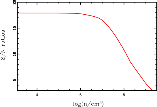
Figure 1: Signal-to-noise ratios pertaining to an AB=13 mag point source versus the surface OH concentrations.

7 Conclusions

We estimate the near-ultraviolet sky background brightness of the lunar exosphere. Our calculations show that the sky brightness is $<8.7\ \mathrm{photon\ s^{-1}\ cm^{-2}\ arcsec^{-2}}$ within the wavelength range 245-340 nm. The signal-to-noise analysis indicates that the detection performance of LUT can be degraded by the sky background emission in most cases. An AB=13 mag point source can be detected by LUT at a signal-to-noise ratio above 8 when the OH concentration is less than $2\times 10^{8}\ \mathrm{molecules\ cm^{-3}}$. However, the effect on the performance is not ignorable when the exosphere is as dense as suggested by CHACE.

References

- Arnold (1979) Arnold, J. R. Ice in the lunar polar regions. JGR 84, 5659-5668, 1979
- Behara & Jeffery (2005) Behara, N. T., Jeffery, C. S. LTE model atmospheres with new opacities. I. Methods and general properties. A&A 451, 643-650, 2005
- Bertaux (1986) Bertaux, J. L. The UV bright spot of water vapor in comets. A&A 160, L7-L10, 1986
- Cao et al. (2011) Cao, L., Ruan, P., Cai, H. B., et al. LUT: A Lunar-based Ultraviolet Telescope. ScChG 54, 558-562, 2011
- Carruthers & Page (1977) Carruthers, G. R., Page, T. Apollo 16 Far-Ultraviolet Camera/Spectrograph: Earth Observations. Science 177, 788-791, 1972
- Carruthers & Page (1977) Carruthers, G. R., Page, T. Apollo-16 far-ultraviolet spectra in the Large Magellanic Cloud. ApJ 211, 728-736, 1977
- Chamberlain & Hunten (1987) Chamberlain, J. W., Hunten, D. M. Theory of Planetary Atmosphere, Academic Press, NewYork, 1987
- Clark (2009) Clark, R. N. Detection of Adsorbed Water and Hydroxyl on the Moon. Science 326, 562-564, 2009
- Crider & Vondrak (2002) Crider, D. H., Vondrak, R. R. Hydrogen migration to the lunar poles by solar wind bombardment of the Moon. AdSpR 30, 1869-1874, 2002
- Crovisier (1989) Crovisier, J. The photodissociation of water in cometary atmospheres. A&A 213, 459-464, 1989
- Dalgarno & Williams (1962) Dalgarno, A., Williams, D. A. Rayleigh Scattering by Molecular Hydrogen. ApJ 136, 690-692, 1962
- Dyar et al. (2010) Dyar, M. D., Hibbitts, C. A., Orlando, T. M. et al. Mechanisms for incorporation of hydrogen in and on terrestrial planetary surfaces. Icar 208, 425-437, 2010
- Feldman et al. (2010) Feldman, P. D., McCandliss, S. R., Morgenthaler, J. P., et al. Galaxy Evolution Explorer Observations of CS and OH Emission in Comet 9P/Tempel 1 During Deep Impact. ApJ 711, 1051-1056, 2010
- Fukugita et al. (1996) Fukugita, M., Ichikawa, T., Gunn, J. E., et al. The Sloan Digital Sky Survey Photometric System. AJ 111, 1748-1756, 1996
- Gullixson (1992) Gullixson, C. A. Two Dimensional Imagery. ASPC 23, 130-159, 1992
- Heiken et al. (1991) Heiken, G. Vaniman, D., French, B. M. LUNAR SOURCEBOOK: A User’s Guide to the Moon I. Cambridge University Press, 1991
- Hibbitts et al. (2010) Hibbitts, C. A., Dyar, M. D., Orlando, T. M., et al. Thermal stability of water and hydroxyl on airless bodies. LPI 41, 2417-2418, 2010
- Hodges (1973) Hodges, Jr. R. R. Helium and hydrogen in the lunar atmosphere. JGR 78(34), 8055-8064, 1973
- Hodges et al. (1972) Hodges, Jr. R. R., Hoffman, J. H., Yeh, T. T. J., et al. Orbital search for lunar volcanism. JGR 73(23), 7307-7317, 1972
- Hunten & Sprague (1997) Hunten, D. M., Sprague, A. L. Origin and character of the lunar and Mercurian atmospheres. AdSpR 19, 1551-1560, 1997
- Johnson & Baragiola (1991) Johnson, R. E., Baragiola, R. Lunar surface - Sputtering and secondary ion mass spectrometry. GeoRL 18, 2169-2172, 1991
- Martin et al. (2005) Martin, D., et al. The Galaxy Evolution Explorer: A Space Ultraviolet Survey Mission, ApJL 619, 1-6, 2005
- Page & Carruthers (1977) Page, T. L., Carruthers, G. R. Apollo 16 far-ultraviolet imagery and spectra of the Large Magellanic Cloud. 1977, Space research XVII; Proceedings of the Open Meetings of Working Groups on Physical Sciences, June 8-19, 1976 and Symposium on Minor Constituents and Excited Species, Philadelphia, Pa., June 9, 10, 1976. (A78-18101 05-42) Oxford and New York, Pergamon Press, 749-755, 1977
- Killen & Ip (1999) Killen, R.M., Ip, W.-H. The surface-bounded atmospheres of Mercury and the Moon. Rev. Geophys 37(3), 361-406., 1999
- Killen et al. (1999) Killen, R. M., Potter, A., Fitzsimmons, A., et al. Sodium D2 line profiles: clues to the temperature structure of Mercury’s exosphere. P&SS 47, 1449-1458, 1999
- Killen et al. (2009) Killen, R., Shemansky, D., Mouawad, N. Expected Emission from mercury exospheric species, and their ultraviolet-visible signatures. ApJS 181, 351-359, 2009
- Merline & Howell (1995) Merline, W. J., Howell, S. B. A Realistic Model for Point-sources Imaged on Array Detectors: The Model and Initial Results. ExA 6, 163-210, 1995
- Morgan & Killen (1997) Morgan, T. H., Killen, R. M. C. A non-stoichiometric model of the composition of the atmospheres of Mercury and the Moon. P&SS 45, 81-94, 1997
- Morgan & Shemansky (1991) Morgan, T. H., Shemansky, D. E. Limits to the Lunar Atmosphere. JGR 96, 1351-1367, 1991
- Morrissey et al. (2005) Morrissey, P., et al. The On-Orbit Performance of the Galaxy Evolution Explorer, ApJL 619, 7-10, 2005
- Mortara & Fowler (1981) Mortara, L., Fowler, A. Evaluations of Charge-Coupled Device CCD Performance for Astronomical Use. SPIE 290, 28-33, 1981
- Pieters et al. (2009) Pieters,C.M., et al. Character and Spatial Distribution of on the Surface of the Moon Seen by M3 on Chandrayaan-1. Science 326, 568-572, 2009
- Schleicher & AHearn (1988) Schleicher, D. G., AHearn, M. F. The fluorescence of cometary OH. ApJ 331, 1058-1077, 1988
- Sneep & Ubachs (2005) Sneep, M., Ubachs, W. Direct measurement of the Rayleigh scattering cross section in various gases. JQSRT 92, 293-310, 2005
- Sridharan et al. (2010a) Sridharan, R., Ahmed, S. M., Pratim. D., et al. Direct’ evidence for water () in the sunlit lunar ambience from CHACE on MIP of Chandrayaan I. P&SS 58, 947-950, 2010
- Sridharan et al. (2010b) Sridharan, R,, Ahmed, S. M., Pratim. D., et al. The sunlit lunar atmosphere: A comprehensive study by CHACE on the Moon Impact Probe of Chandrayaan-1. P&SS 58, 1567-1577, 2010
- Starukhina & Shkuratov (2000) Starukhina,L.V., Shkuratov,Y.G. NOTE: The Lunar Poles: Water Ice or Chemically Trapped Hydrogen? Icar 147, 585-587, 2000
- Starukhina & Shkuratov (2010) Starukhina,L.V., Shkuratov,Y.G. Simulation of 3-m Absorption Band in Lunar Spectra: Water or Solar Wind Induced Hydroxyl? LPI 41, 1385-1386, 2010
- Stern (1999) Stern, S. A. The lunar atmosphere: History, status, current problems, and context. RvGeo 37, 453-492, 1999
- Stern et al. (1997) Stern, S. A., Parker, J. W., Morgan, T. H., et al. NOTE: an HST Search for Magnesium in the Lunar Atmosphere. ICARUS 127, 523-526, 1997
- Stubbs et al. (2010) Stubbs, T. J., Glenar, D. A., Colaprete, A., et al. Optical scattering processes observed at the moon: Predictions for the LADEE ultraviolet spectrometer. P&SS 58, 830-837, 2010
- Sunshine et al. (2009) Sunshine,J. M., Farnham, T. L., Feaga, L. M., et al. Temporal and Spatial Variability of Lunar Hydration As Observed by the Deep Impact Spacecraft. Science 326, 565-568, 2009
- Tarafdar & Vardya (1973) Tarafdar, S. P., Vardya, M. S. The importance of molecular Rayleigh scattering in the atmospheres of very late type stars. MNRAS 163, 261-277, 1973
- Wurz et al. (2007) Wurz, P., Rohner, U., Whitby, J. A., et al. The lunar exosphere: The sputtering contribution. ICARUS 191, 486-496, 2007