FTUAM-11-46  IFT-UAM/CSIC-11-27
Neutrino masses in $SU(5)\times U(1)_{F}$ with adjoint flavons

Abstract

We present a $SU(5)\times U(1)_{F}$ supersymmetric model for neutrino masses and mixings that implements the seesaw mechanism by means of the heavy $SU(2)$ singlets and triplets states contained in three adjoints of $SU(5)$. We discuss how Abelian $U(1)_{F}$ symmetries can naturally yield non-hierarchical light neutrinos even when the heavy states are strongly hierarchical, and how it can also ensure that $R$–parity arises as an exact accidental symmetry. By assigning two flavons that break $U(1)_{F}$ to the adjoint representation of $SU(5)$ and assuming universality for all the fundamental couplings, the coefficients of the effective Yukawa and Majorana mass operators become calculable in terms of group theoretical quantities. There is a single free parameter in the model, however, at leading order the structure of the light neutrinos mass matrix is determined in a parameter independent way.

1 Introduction

The standard model (SM) is a very successful framework for describing particle physics phenomena. However, it suffers from some serious theoretical problem, among which: neutrinos are massless, the conditions for baryogenesis are not fulfilled, and there is no candidate for the dark matter (DM). The first two problems can be solved by extending the SM to include the seesaw mechanism for neutrino masses [1, 2, 3, 4, 5] that also opens the possibility of baryogenesis via leptogenesis [6, 7], while extending the SM to its supersymmetric version (SSM) can provide a natural candidate for DM. However, in contrast to the SM, the SSM does not have accidental lepton ($L$) and baryon-number ($B$) symmetries, and this can lead to major phenomenological problems, like fast proton decay. The standard solution to forbid all dangerous operators is to impose a discrete symmetry, $R$–parity, and only in the $R$-parity conserving SSM the lightest supersymmetric particle (LSP), generally the neutralino, is stable, and provides a good DM candidate.

Similarly to the SM, also the SSM does not provide any explanation for the strong hierarchy in the fermion Yukawa couplings. One way to explain the flavor puzzle and the suppression of the fermion masses with respect to the electroweak breaking scale is to impose Abelian flavor symmetries, that we generically denote as $U(1)_{F}$, that are broken by SM-singlets commonly denoted as flavons. Besides the Yukawa couplings, these symmetries can also suppress, but often not forbid completely, the SSM $B$ and $L$ violating terms. Along these lines, consistent models can be build in which small neutrino masses can be accommodated (for a review see [8]). Due to the fact that in these models $R$–parity is not an exact symmetry, the LSP can decay, however, long lived LSP can also provide acceptable DM candidates [9].

When $R$ parity is not imposed, there is also the possibility that it could arise as an accidental symmetry like it happens in the SM for $B$ and $L$. $R$-parity conservation can be for example enforced by an extended gauge symmetry together with supersymmetry (that requires a holomorphic superpotential) as in the model studied in [10], or solely by the gauge symmetry thanks to a suitable choice of the $U(1)_{F}$–charges, as in ref. [11]. In this paper we focus on this second possibility, and we implement it in the framework of a unified $SU(5)\times U(1)_{F}$ model. A virtue of the $U(1)_{F}$ gauge symmetry of our model is that when the $U(1)_{F}$ charges are chosen appropriately, $\Delta B\neq 0$ and $\Delta L=1$ operators are forbidden at all orders. However, $\Delta L=2$ operators corresponding to Majorana masses for heavy neutral fermions of the seesaw remain allowed, and thus the seesaw mechanism can be embedded in the model. More in detail, following [11] we chose the $F$-charges in such a way that operators with even $R$–parity have an overall $F$-charge that is an integer multiple of the charge of the $U(1)_{F}$ breaking scalar fields (that, without loss of generality, we set equal to $\pm 1$). In contrast, all the $R$–parity breaking operators, that have an overall half-odd-integer $F$–charge, are forbidden. Then, to allow for $\Delta L=2$ Majorana masses while forbidding $\Delta L=1$ operators, it is sufficient to chose the $F$–charges of the heavy seesaw neutral states as half–odd-integers.

Differently from the SM case [11], in $SU(5)$ GUTs it is rather difficult to implement this kind of horizontal symmetries, because there is less freedom in choosing the $F$–charges (see for example [12]). However, if the flavons that break the horizontal symmetry are assigned to the adjoint representation of $SU(5)$ [13, 14, 15], charges that were forbidden in the singlet flavon case become allowed, under the assumption that certain representations for the Froggatt-Nielsen (FN) [16] messengers fields do not exist. In contrast to the non-unified $SU(3)\times SU(2)\times U(1)\times U(1)_{F}$ model, where the singlet nature of the flavons is mandatory, in $SU(5)\times U(1)_{F}$ assigning the flavons to the adjoint has the additional bonus that non-trivial group theoretical coefficients concur to determine the coefficients of the effective operators [13, 14, 15]. In this case, under the additional assumption that at the fundamental level all the Yukawa couplings obey to some principle of universality [14], the order one coefficients that determine quantitatively the structure of the mass matrices become calculable. In this paper we will avoid all speculations concerning the fundamental physics that might underlie such a universality principle; we just take it as a convenient working hypothesis: turning off the ‘noise’ related to the usual incalculable order one Yukawa couplings allows to put in clear the role played by the calculable group theoretical coefficients that multiply all the relevant effective operators.

2 Theoretical framework

2.1 Same sign and both signs Abelian charges

Sometimes symmetry considerations are sufficient to determine univocally the structure of the low energy operators, however, other times a detailed knowledge of the full high energy theory is needed. Let us consider for example a $U(1)_{F}$ symmetry and assume that all the heavy and light states have charges of the same sign, say positive. Then a single spurion $\epsilon_{-1}$ with a negative unit charge is involved in the construction of all $U(1)_{F}$ (formally) invariant operators. Let us consider the ${\rm dim}=5$ seesaw operator ${\cal L}_{D5}\sim-\frac{g_{\alpha\beta}}{2\,M}\left(\bar{\ell}_{\alpha}H\right)\left(H^{T}\ell^{c}_{\beta}\right)$, where $\ell_{\alpha}$ are the lepton doublets and $H$ is the Higgs field, that for simplicity we take neutral under the Abelian symmetry $F(H)=0$. Since the only spurion useful to construct (formally) invariant operators is $\epsilon_{-1}$, one can easily convince himself that the structure of $g_{\alpha\beta}$, and thus the structure of the light neutrino mass matrix, is univocally determined by the $F$ charges of the light leptons as: $g_{\alpha\beta}\sim\epsilon_{-1}^{F(\ell_{\alpha})+F(\ell_{\beta})}$, while the $F$-charges of whatever heavy states of mass $\sim M$ are inducing the effective operator are irrelevant. We can conclude that in this case one does not need to consider the details of the high energy theory, since the structure of the low energy effective operators can be straightforwardly read off from the charges of the light states.

However, if we allow for $U(1)_{F}$ charges of both signs, then both symmetry breaking spurions $\epsilon_{-1}=\epsilon_{+1}=\epsilon$ are relevant. This implies that naive charge counting applied to the low energy effective operators is unreliable, since basically a factor $\epsilon^{n}$, as estimated in the low energy theory, could correspond instead to $\epsilon^{n+m}_{+1}\cdot\epsilon^{m}_{-1}\sim\epsilon^{n+2m}$. Clearly the naive estimate can result in a completely different (and wrong) structure with respect to the one effectively generated by the high energy theory. We illustrate this with a simple example: let us take two lepton doublets with charges $F(\ell_{1})=-F(\ell_{2})=+1$ and again $F(H)=0$. The structure of the light neutrino mass matrix read off from the lepton doublets charges would be given by the low energy coefficient:

$$g_{\alpha\beta}\sim\begin{pmatrix}\epsilon^{2}&1\\ 1&\epsilon^{2}\end{pmatrix}\,.$$ (1)

This corresponds to a pair of quasi degenerate (pseudo-Dirac) light neutrinos.

Now, let us assume that the fundamental high energy (seesaw) theory has two right handed neutrinos with charges $F(N_{1,2})=+1$. For the heavy mass matrix $M_{N}$, its inverse, and for the Yukawa coupling $Y_{\alpha i}\bar{\ell}_{\alpha}N_{i}$ we obtain:

$$M_{N} \sim\epsilon^{2}\begin{pmatrix}1&1\\ 1&1\end{pmatrix}\,, M_{N}^{-1} \sim\epsilon^{-2}\begin{pmatrix}1&1\\ 1&1\end{pmatrix}\,, Y \sim\begin{pmatrix}1&1\\ \epsilon^{2}&\epsilon^{2}\end{pmatrix}\,.$$ (2)

The resulting effective low energy coefficient is:

$$g_{\alpha\beta}\sim YM_{N}^{-1}Y^{T}\sim\epsilon^{-2}\begin{pmatrix}1&\epsilon^{2}\\ \epsilon^{2}&\epsilon^{4}\end{pmatrix}\,,$$ (3)

which (for $\epsilon\ll 1$) corresponds to very hierarchical and mildly mixed light neutrinos, that is a completely different result from the previous one.

The model we are going to describe in this paper requires fermions with charges of both signs, as well as a pair of positively and negatively charged spurions. Therefore a detailed knowledge of the high energy theory is mandatory, and accordingly we will explicitly describe all its relevant aspects.

2.2 Outline of the $SU(5)\times U(1)_{F}$ model

We assume that at the fundamental level all the Yukawa couplings are universal, and that all the heavy messengers states carrying $U(1)_{F}$ charges have the same mass, as it would happen if the masses are generated by the vacuum expectation values (vev) of some singlet scalar. With these assumptions, the only free parameter of the model is the ratio between the vacuum expectation value of the flavons and the mass of the heavy vectorlike FN fields. This parameter is responsible for the fermion mass hierarchy, and all the remaining features of the mass spectrum are calculable in terms of group theoretical coefficients. More precisely, in our model the flavor symmetry is broken by vevs of scalar fields $\langle\Sigma_{\pm}\rangle$ in the $\mathbf{24}$–dimensional adjoint representation of $SU(5)$, where the subscripts refer to the values $\pm 1$ of the $U(1)_{F}$ charges that set the normalization for all the other charges. The vevs $\langle\Sigma_{+}\rangle=\langle\Sigma_{-}\rangle=V_{a}$ with $V_{a}=V\cdot\operatorname{diag}(2,2,2,-3,-3)/\sqrt{60}$ are also responsible for breaking the GUT symmetry down to the electroweak–color gauge group. The size of the order parameters breaking the flavor symmetry is then $\epsilon=V/M$ where $M$ is the common mass of the heavy FN vectorlike fields. This symmetry breaking scheme has two important consequences: power suppression in $\epsilon$ appear with coefficients related to the different entries in $V_{a}$, and the FN fields are not restricted to the $\mathbf{5}$, $\overline{\mathbf{5}}$, or $\mathbf{10}$, $\overline{\mathbf{10}}$, multiplets as is the case when the $U(1)_{F}$ breaking is triggered by singlet flavons [13, 14].

The model studied in [14] adopted this same scheme, and yields a viable phenomenology, since it produces quark masses and mixings and charged lepton masses that are in agreement with the data. The $U(1)_{F}$ charge assignments of the model yield $U(1)_{F}$ mixed anomalies, that are canceled trough the Green-Schwartz mechanism [17]. The values of the charges are determined only modulo an overall rescaling, that may be appropriately chosen in order to forbid baryon and lepton number violating couplings. However, with the choice of charges adopted in [14], both $\Delta L=1$ and $\Delta L=2$ violating operators were forbidden, and thus the seesaw mechanism could not be embedded in the model. In order to avoid this unpleasant feature, in this work we explore the possibility of forbidding just the $\Delta L=1$ operators while allowing the $\Delta L=2$ seesaw operator for neutrino masses. We will show that by means of a suitable choice of the $F$ charges, the seesaw mechanism can be implemented, and one can obtain neutrino masses and mixings in agreement with oscillation data, while $\Delta L=1$ and $\Delta B\neq 0$ (and thus $R$–parity violating) operators are forbidden at all orders by virtue of the $F$-charges. Moreover, the scale of the heavy seesaw neutral fermions remains fixed, and lies a few order of magnitude below the GUT scale, and is of the right order to allow the generation of the baryon asymmetry through leptogenesis.

2.3 Charge assignments

The $F$ charges have to satisfy some specific requirements in order to yield a viable phenomenology. In the following we denote for simplicity the various $F$ charges with the same label denoting the corresponding $SU(5)$ multiplet. To allow a Higgsino $\mu$–term at tree level, we must require

$$\overline{\mathbf{5}}^{\phi_{d}}+\mathbf{5}_{\phi_{u}}=0\,,$$ (4)

where $\overline{\mathbf{5}}^{\phi_{d}},\,\mathbf{5}_{\phi_{u}}$ denote the $F$-charges of the chiral multiplets containing the $SU(2)$ Higgs doublets $\phi_{d},\,\phi_{u}$. It is easy to see that with the constraint (4) the overall charge of the Yukawa operators for the charged fermion masses $\mathbf{10}_{I}\mathbf{\bar{5}}_{J}\mathbf{\bar{5}}^{{\phi}_{d}}$ and $\mathbf{10}_{I}\mathbf{10}_{J}\mathbf{{5}}_{{\phi}_{u}}$, that are even under $R$–parity, are invariant under the charge redefinitions [14]:

$$\mathbf{\bar{5}}_{I} \to\mathbf{\bar{5}}_{I}+a_{n}$$ (5)

$$\mathbf{10}_{I} \to\mathbf{10}_{I}-\frac{a_{n}}{3}$$

$$\mathbf{\bar{5}}^{{\phi}_{d}} \to\mathbf{\bar{5}}^{{\phi}_{d}}-\frac{2a_{n}}{3}$$

$$\mathbf{5}_{{\phi}_{u}} \to\mathbf{5}_{{\phi}_{u}}+\frac{2a_{n}}{3}\,,$$

where $I=1,2,3$ is a generation index, and $a_{n}$ is an arbitrary parameter that can be used to redefine the charges. Assuming $\mathbf{5}_{\phi_{u}}=0$, then the anomalous solution that was chosen in ref. [14] can be written as

$$\mathbf{5}_{\phi_{u}}=\overline{\mathbf{5}}^{\phi_{d}}= 0\,, \overline{\mathbf{5}}_{I}=2^{I}-7\,, \mathbf{10}_{I}=3-I\,.$$ (6)

Starting from a set of integer charges, and redefining this set by means of the shift eq. (5) with

$$a_{n}=-\frac{3}{2}\left(\frac{2n}{5}+1\right)\,,$$ (7)

where $n$ is an integer, it is easy to see that the $R$–parity violating operators $\mathbf{10}_{I}\mathbf{\bar{5}}_{J}\mathbf{\bar{5}}_{K}$ and $\mathbf{\bar{5}}_{I}\mathbf{{5}}_{{\phi}_{u}}$ have half–odd–integer charges, and hence are forbidden at all orders by the $U(1)_{F}$ symmetry.

To generate neutrino masses, we now introduce three heavy multiplets $\mathbf{N}_{I}$ $(I=1,2,3$) with half–odd–integer $F$–charges, that we assume corresponding to adjoint representations $\mathbf{24}$. The adjoint of $SU(5)$ contains two types of $SU(2)$ multiplets that can induce at low energy the dimension five Weinberg operator [18]: one $SU(2)\times U(1)\times SU(3)$ singlet that allows to implement the usual type I seesaw, and one $U(1)\times SU(3)$ singlet but $SU(2)$ triplet giving rise to a type III seesaw [19, 20, 21]. Contributions from these two types of multiplets unavoidably come together, so that by assigning ‘right handed neutrinos’ to the $\mathbf{24}$ of $SU(5)$ one necessarily ends up with a type I+III seesaw. This slightly more complicated seesaw structure is not crucial for our construction, but we still keep track of it for a matter of consistency.

The half–odd–integer charges of the new states, after the charges of the other fields have been shifted according to eqs. (5) and (7), can be parameterized as

$$N_{I}=\frac{2m_{I}+1}{2}\,,$$ (8)

where $m_{I}$ are integers. The effective superpotential terms that give rise to the seesaw are

$$W_{\text{seesaw}}=Y_{\nu}^{IJ}\,\overline{\mathbf{5}}_{I}\,\mathbf{5}_{\phi_{u}}\,\mathbf{N}_{J}+\tfrac{1}{2}M_{R}^{IJ}\mathbf{N}_{I}\mathbf{N}_{J}\,.$$ (9)

The coefficient $Y_{\nu}^{IJ}$ of the Dirac operator in eq. (9) is determined by the following sums of $F$–charges:

$$\overline{\mathbf{5}}_{I}+\mathbf{5}_{\phi_{u}}+\mathbf{N}_{J}= 2^{I}-7+a_{n}+2a_{n}/3+N_{J}$$

$$= 2^{I}-9+n+m_{J}\,.$$

Explicitly:

$$F(\overline{\mathbf{5}}_{I}\,\mathbf{5}_{\phi_{u}}\,\mathbf{N}_{J})= \begin{pmatrix}-7-n+m_{1}&-7-n+m_{2}&-7-n+m_{3}\\ -5-n+m_{1}&-5-n+m_{2}&-5-n+m_{3}\\ -1-n+m_{1}&-1-n+m_{2}&-1-n+m_{3}\\ \end{pmatrix}.$$ (10)

For the mass operator of the adjoint neutrinos we have the following (integer) $F$–charges

$$\mathbf{N}_{I}+\mathbf{N}_{J}= 1+m_{I}+m_{J}\,,$$

$$F(\mathbf{N}_{I}\,\mathbf{N}_{J})= \begin{pmatrix}1+2m_{1}&1+m_{1}+m_{2}&1+m_{1}+m_{3}\\ 1+m_{1}+m_{2}&1+2m_{2}&1+m_{2}+m_{3}\\ 1+m_{1}+m_{3}&1+m_{2}+m_{3}&1+2m_{3}\\ \end{pmatrix}.$$ (11)

The light neutrino mass matrix is then obtained from the seesaw formula

$$M_{\nu}\approx -{v^{2}}\sin^{2}\beta\,Y_{\nu}\,M_{R}^{-1}\,Y^{T}_{\nu}\,,$$ (12)

where $v=175\,$GeV, and it is left understood that in eq. (12) the contributions of the $SU(2)$ singlets and triplets are both summed up. As is implied by the FN mechanism, the order of magnitude of the entries in $Y_{\nu}$ and $M_{R}$ is determined by the corresponding values of the sums of $F$ charges eqs. (10) and (2.3) as:

$$Y_{\nu}^{IJ} \sim\epsilon^{|\overline{\mathbf{5}}_{I}+\mathbf{5}_{\phi_{u}}+\mathbf{N}_{J}|}$$

$$M_{R}^{IJ} \sim M\cdot\epsilon^{|\mathbf{N}_{I}+\mathbf{N}_{J}|}=V\cdot\epsilon^{|\mathbf{N}_{I}+\mathbf{N}_{J}|-1}\,.$$ (13)

where in the second relation $M$ is the mass of the FN messengers fields and in the last equality we have used $M=\epsilon^{-1}V$. Note that since we have two flavon multiplets $\Sigma_{\pm}$ with opposite charges, the horizontal symmetry allows for operators with charges of both signs, and hence the exponents of the symmetry breaking parameter $\epsilon$ in eq. (2.3) must be given in terms of the absolute values of the sum of charges. In FN models only the order of magnitude of the entries in eq. (2.3) are determined, and it is generally assumed that non-hierarchical order one coefficients multiply each entry. However, in our model the assumption of universality for the fundamental Yukawa couplings has been made in order to avoid arbitrary $\mathcal{O}(1)$ numbers of unspecified origin. The coefficients multiplying each entry in eq.(2.3) can be in fact computed with the same technique introduced in [14] for computing the down-quark and charged lepton masses. In summary, the order of magnitude of the various entries in $M_{\nu}$ is determined by the appropriate powers of the small factor $\epsilon$ while, as we will see, the details of the mass spectrum are determined by non-hierarchical computable group theoretical coefficients, that only depend on the way the heavy FN states are assigned to $SU(5)$ representations.

2.4 Coefficients of the Dirac and Majorana effective operators

In this section we analyze the contributions of different effective operators to $Y_{\nu}$ and to $M_{R}$, showing that a phenomenologically acceptable structure, able to reproduce (approximately) the correct mass ratios and to give reasonable neutrino mixing angles can be obtained.

We assume that a large number of vectorlike FN fields exist in various $SU(5)$ representations. Since we assign the heavy Majorana neutrinos to the adjoint $\mathbf{N}$, the possible FN field representations $\mathbf{R}$ can be identified starting from the following tensor products involving the representations of the fields in the external lines (see the diagrams in Fig. 1):

$$\mathbf{\overline{5}\otimes{5_{\phi_{u}}}}= \mathbf{{1}\oplus{24}}\,,$$ (14)

$$\mathbf{\overline{5}}\>\>\mathbf{\otimes}\>\>\mathbf{\Sigma}\ = \mathbf{\overline{5}\oplus\overline{45}\oplus\overline{70}}\,,$$ (15)

$$\mathbf{{N}\>\otimes{\Sigma}}\>\>= \mathbf{{1_{S}}}\oplus\mathbf{{24_{S}}}\oplus\mathbf{24_{A}}\oplus\mathbf{{75_{S}}}\oplus\mathbf{{126_{A}}}$$

$$\oplus\mathbf{\overline{126_{A}}}\oplus\mathbf{{200_{S}}}\,,$$ (16)

where the subscripts $\scriptstyle\mathbf{S,\,A}$ in the last line denote the symmetric or antisymmetric nature of the corresponding representations. We assume that all FN fields transform nontrivially under $SU(5)$, and thus that no singlet exists and, for simplicity, we restrict ourselves to representations with dimension less than 100, which results in the following possibilities $\mathbf{R}=\mathbf{24}$, $\mathbf{5}$, $\mathbf{45}$, $\mathbf{70}$.

Pointlike propagators: Since the mass $M$ of these fields is assumed to be larger than $\langle\Sigma_{\pm}\rangle\sim\Lambda_{\text{GUT}}$, the contributions to the operators in eq. (9) can be evaluated by means of insertions of effective pointlike propagators. As in [14] we denote the contractions of two vectorlike fields in the representation $\mathbf{R}$, $\overline{\mathbf{R}}$ as

$$\left[\mathbf{R}_{de\ldots}^{abc\ldots}\overline{\mathbf{R}}_{lmn\ldots}^{pq\ldots}\right]=-\frac{i}{M}\mathcal{S}_{de\ldots lmn\ldots}^{abc\ldots pq\ldots}\,,$$ (17)

where all the indices are $SU(5)$ indices, and $\mathcal{S}$ is the appropriate group index structure. The structures $\mathcal{S}$ for $\left[\mathbf{5}^{a}\,\mathbf{\bar{5}}_{b}\right]$, $\left[\mathbf{45}^{ab}_{c}\,\mathbf{\bar{45}}^{n}_{lm}\right]$ and $\left[\mathbf{70}^{ab}_{c}\,\mathbf{\bar{70}}^{n}_{lm}\right]$ (and for several other $SU(5)$ representations) can be found in Appendix A of [14]. In addition we need the following contractions

$$iM\left[\mathbf{24}^{a}_{b}\,\mathbf{24}^{l}_{m}\right]_{\mathbf{S}} =\left({\cal S}_{\mathbf{S}}\right)^{a\,l}_{b\,m}=\frac{5}{2}\left[\delta^{a}_{m}\,\delta_{b}^{l}+\delta^{a}_{l}\,\delta_{b}^{m}\right]-\delta^{a}_{b}\,\delta_{m}^{l}\,,$$ (18)

$$iM\left[\mathbf{24}^{a}_{b}\,\mathbf{24}^{l}_{m}\right]_{\mathbf{A}} =\left({\cal S}_{\mathbf{A}}\right)^{a\,l}_{b\,m}=\frac{5}{2}\left[\delta^{a}_{m}\,\delta_{b}^{l}-\delta^{a}_{l}\,\delta_{b}^{m}\right]\,.$$ (19)

These two expressions are obtained by imposing the traceless condition for the adjoint $\left({\cal S}_{\mathbf{S,A}}\right)^{a\,l}_{a\,m}=\left({\cal S}_{\mathbf{S,A}}\right)^{a\,l}_{b\,l}=0$ and the normalization factor is fixed by the requirement that the (subtracted) singlet piece $\delta^{a}_{b}\,\delta_{m}^{l}$ in eq. (18) provides the proper singlet contraction, that is, by inserting the singlet in the diagram of fig.1(b) we require that the operator $\left(\mathbf{\overline{5}}_{a}\mathbf{5}_{\phi_{u}}^{a}\right)\cdot\left(\mathbf{N}_{l}^{j}\mathbf{\Sigma}_{j}^{l}\right)$ is obtained with unit coefficient.

Vertices:  All the vertices we need involve $\mathbf{5}_{\phi_{u}}$ or the adjoint $\mathbf{\Sigma}$ with the external fermions $\mathbf{\bar{5}}$ and $\mathbf{N}$, or with the FN representations $\mathbf{R}$ in the internal lines. The vertices have the general form $-i\lambda{\cal V}$ where $\lambda$ is universal for all vertices. Including symmetry factors, the relevant field contractions ${\cal V}=\mathbf{R}\,\mathbf{5}_{\phi_{u}}\,\mathbf{R^{\prime}}$ or ${\cal V}=\mathbf{R}\,\mathbf{\Sigma}\,\mathbf{R^{\prime}}$, with $\mathbf{R},\mathbf{R^{\prime}}=\mathbf{5},\,\mathbf{24},\,\mathbf{45},\,\mathbf{70}$, are:

$$\mathbf{\bar{5}}_{a}\mathbf{24}^{a}_{b}\mathbf{5}^{b}\qquad\!\!\!\mathbf{\bar{5}}_{a}\mathbf{24}^{c}_{b}\mathbf{45}^{ba}_{c}\qquad\!\!\!\mathbf{\bar{5}}_{a}\mathbf{24}^{c}_{b}\mathbf{70}^{ba}_{c}\qquad\mathbf{24}^{a}_{c}\mathbf{24}^{c}_{b}\left(\mathbf{24}_{\mathbf{S,A}}\right)^{b}_{a}.$$ (20)

$$\mathbf{\bar{45}}_{ab}^{c}{\mathbf{24}^{\uparrow}}^{b}_{d}\mathbf{45}^{da}_{c}\quad\ \quad\frac{1}{2}\,\mathbf{\bar{45}}_{ab}^{c}{\mathbf{24}^{\downarrow}}_{c}^{d}\mathbf{45}^{ba}_{d}$$ (21)

$$\mathbf{\bar{70}}_{ab}^{c}{\mathbf{24}^{\uparrow}}^{b}_{d}\mathbf{70}^{da}_{c}\quad\ \quad\frac{1}{2}\,\mathbf{\bar{70}}_{ab}^{c}{\mathbf{24}^{\downarrow}}_{c}^{d}\mathbf{70}^{ba}_{d}\quad\ \quad\mathbf{\bar{45}}_{ab}^{c}\mathbf{24}^{b}_{d}\mathbf{70}^{da}_{c}\,,$$ (22)

where the vertices in the first line describe the couplings of the external states ($\mathbf{\overline{5}}$ and $\mathbf{N}$) with heavy FN fields and flavons, while the last two lines involve only heavy FN fields and flavons. There are two inequivalent ways of contracting the indices for the vertices involving the $\mathbf{24}$ with pairs of $\mathbf{45}$ and $\mathbf{70}$ in the last two lines [14]. They are distinguished in eqs. (21) and (22) by an up ($\mathbf{24}^{\uparrow}$) or down ($\mathbf{24}^{\downarrow}$) arrow-label. As explained in [14], this can be traced back to the fact that these representations are contained twice in their tensor products with the adjoint.

Relevant multiplet components: We write the $SU(5)\times U(1)_{F}$ breaking vevs as

$$\langle\mathbf{\Sigma_{\pm}}\rangle=\frac{V}{\sqrt{60}}\times\operatorname{diag}(2,2,2,-3,-3)\,,$$ (23)

where the factor $1/\sqrt{60}$ gives the usual normalization of the $SU(5)$ generators, $\operatorname{Tr}(\mathbf{R}^{a}\overline{\mathbf{R}^{b}})=(1/2)\delta^{ab}$, and the coefficients of the left handed neutrino couplings to the $SU(2)$ singlet $\nu\,\phi^{0}_{u}\,N_{S}$ and $SU(2)$ triplet $\nu\,\phi^{0}_{u}\,N_{T}$ as well as the Majorana neutrinos mass terms $N_{S,T}\,N_{S,T}$ are obtained by projecting the representations $\mathbf{5}$, $\mathbf{5}_{\phi_{u}}$ and $\mathbf{N}$ onto the relevant field components according to

$$\nu = -\overline{\mathbf{5}}_{5}=-\delta_{5}^{a}\;\overline{\mathbf{5}}_{a}$$ (24)

$$\phi^{0}_{u} = \mathbf{5}_{\phi_{u}}^{5}=\delta^{5}_{b}\;\mathbf{5}_{\phi_{u}}^{b}$$ (25)

$$N_{S} = \frac{1}{\sqrt{60}}\;\operatorname{diag}(2,\,2,\,2,\,-3,\,-3)\cdot\mathbf{N}_{24}\,.$$ (26)

$$N_{T} = \frac{1}{\sqrt{60}}\;\operatorname{diag}(0,\,0,\,0,\,\sqrt{15},\,-\sqrt{15})\cdot\mathbf{N}_{3}\,.$$ (27)

where the subscripts in $\mathbf{N}_{24}$ (singlet) and $\mathbf{N}_{3}$ (neutral component of the triplet) refer to the corresponding $SU(5)$ generators. The assumption of a unique heavy mass parameter $M$ for the FN fields and of universality of the fundamental scalar-fermion couplings $\lambda$ yield a remarkable level of predictivity. In particular, for the vertices involving $\mathbf{\Sigma_{\pm}}$ we can always reabsorb $\lambda V\to V$. This leaves just an overall power of $\lambda$ common to all effective Yukawa operators that involve one insertion of the Higgs multiplet $\mathbf{5}_{\phi_{u}}$ (see the diagrams in Figs. 1) and no $\lambda$ at all for the contributions to $M_{R}$, (see the diagrams in Figs. 2).

The contributions to $Y_{\nu}$ and $M_{R}$ at different orders can be computed using the vertices $\mathcal{V}$ given in eqs. (20)-(22) and the relevant group structures $\mathcal{S}$ in eqs. (18), (19) and in Appendix A of [14], that account for integrating out the heavy FN fields. Additionally, the multiplets $\mathbf{\bar{5}}$, $\mathbf{N}$, and $\mathbf{5}_{\phi_{u}}$ in the external legs of the diagrams must be projected on the relevant components according to eqs. (24)-(27) and the flavons $\mathbf{\Sigma_{\pm}}$ have to be projected onto the vacuum according to eq. (23).

We have evaluated the $Y_{\nu}$ including the contributions up to $\mathcal{O}(\epsilon^{2})$ that are diagrammatically depicted in Figs. 1: 1(a) $\mathcal{O}(\epsilon^{0})$; 1(b)–1(c) $\mathcal{O}(\epsilon^{1})$; 1(d)–1(f) $\mathcal{O}(\epsilon^{2})$. $M_{R}$ has been computed including contributions with three insertions of the flavons $\Sigma_{\pm}$ corresponding to the diagrams in Figs. 2: 2(a) $\mathcal{O}(\epsilon)$; 2(b) $\mathcal{O}(\epsilon^{2})$; 2(c) $\mathcal{O}(\epsilon^{3})$. At each specific order, the contributions to specific entries in $Y_{\nu}$ and $M_{R}$ can be written as

$$Y_{\nu}^{(i)} = \lambda\,\alpha^{i+1}\,\epsilon^{i}\cdot\left(y^{S}_{i}+y^{T}_{i}\right)\,,$$ (28)

$$M_{R}^{(i)} = V\,\alpha^{i+3}\,\epsilon^{i}\cdot\left(r^{S}_{i+1}+r^{T}_{i+1}\right)=M\,\alpha^{i+3}\,\epsilon^{i+1}\cdot\left(r^{S}_{i+1}+r^{T}_{i+1}\right)\,,$$ (29)

where $\alpha=1/\sqrt{60}$ is the normalization factor for $\mathbf{\Sigma}$ and for the $N_{S,T}$ in the adjoint, $V=M\epsilon$ with $V$ defined in eq. (23), and $y_{i}^{S,T}$ and $r_{i+1}^{S,T}$ are the nontrivial group theoretical coefficients, that we have computed for $i=0,1,2$ and for the singlet $(S)$ and triplet $(T)$ contributions to the seesaw Lagrangian. The corresponding results for $y_{i}^{S,T}$ are given in Table 2 (where we have followed the notation of [14]), while the results for $r_{i+1}^{S,T}$ are given in Table 3.

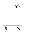
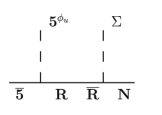
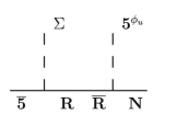
                     (a)                                               (b)                                               (c)

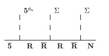
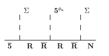
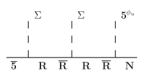
                       (d)                                              (e)                                             (f)

Figure 1: Diagrams contributing to $Y_{\nu}$ at different orders. The lowest order coefficient corresponding to diagram (a) is $y_{0}=3$. Diagrams (b)–(c) contribute at ${\cal O}(\epsilon^{1})$ and yield the coefficients $y_{1}$ in the second column in Table 2. Diagrams (d)–(f) contribute at ${\cal O}(\epsilon^{2})$ and give the coefficients $y_{2}$ in the fourth column of the table.

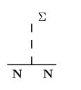
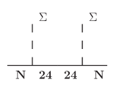
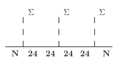
              (a)                                         (b)                                                      (c)

Figure 2: Diagrams contributing to $M_{R}$ at different orders. The lowest order coefficient $r_{1}$ is obtained from diagram (a), $r_{2}$ from (b), and $r_{3}$ from (c).

$\mathbf{\bar{5}}_{1}$	$\mathbf{\bar{5}}_{2}$	$\mathbf{\bar{5}}_{3}$	$\mathbf{10}_{1}$	$\mathbf{10}_{2}$	$\mathbf{10}_{3}$	$\mathbf{5}_{\phi_{u}}=-\mathbf{5}_{\phi_{d}}$	$N_{1}$	$N_{2}$	$N_{3}$
$-\frac{29}{10}$	-$\frac{9}{10}$	$\frac{31}{10}$	$\frac{13}{10}$	$\frac{3}{10}$	$-\frac{7}{10}$	$\frac{7}{5}$	$\frac{5}{2}$	$-\frac{1}{2}$	$-\frac{11}{2}$

Table 1: $F$–charges obtained with $n=-6$ in eq. (7), and $m_{1}=2$, $m_{2}=-1$, and $m_{3}=-6$ in eq. (8).

We have searched for all possible charge assignments with absolute values of the $F$ charges smaller than 10, and we have examined the resulting neutrino mass matrices. We have found some promising possibilities. If we choose, for example, in eqs. (10) and (2.3), $n=-6$ and $m_{1}=2$, $m_{2}=-1$, $m_{3}=-6$, we obtain the $F$–charges shown in Table 1, which can be obtained from the set given in eq. (6) through the redefinitions eqs. (5) with $a_{-6}=21/10$.

According to eq. (10), this set of $F$–charges gives the following orders of magnitude for $Y_{\nu}$:

$$Y_{\nu}\sim \lambda\begin{pmatrix}\epsilon&\epsilon^{2}&\epsilon^{7}\\ \epsilon^{3}&1&\epsilon^{5}\\ \epsilon^{7}&\epsilon^{4}&\epsilon\\ \end{pmatrix}.$$ (30)

Neglecting terms of $\mathcal{O}(\epsilon^{4})$ and higher, including the coefficients $y_{i}^{S,T}$ and the appropriate powers of the normalization factor $\alpha$, this reads:

$$Y_{\nu}^{S,T}\,\approx\, \lambda\,\alpha\,\begin{pmatrix}y_{1}(\alpha\epsilon)&y_{2}(\alpha\epsilon)^{2}&0\\ y_{3}(\alpha\epsilon)^{3}&y_{0}&0\\ 0&0&y_{1}(\alpha\epsilon)\\ \end{pmatrix}^{S,T}.$$ (31)

where the superscript ^S,T outside the matrix is a shorthand for $y_{i}^{S,T}$ inside the matrix. Similarly, according to eq. (2.3) and (2.3) we have for the entries in $M_{R}$ the following orders of magnitude:

$$M_{R}\,\sim\, V\,\begin{pmatrix}\epsilon^{4}&\epsilon^{1}&\epsilon^{2}\\ \epsilon^{1}&\epsilon^{0}&\epsilon^{5}\\ \epsilon^{2}&\epsilon^{5}&\epsilon^{10}\\ \end{pmatrix}.$$ (32)

Neglecting terms of $\mathcal{O}(\epsilon^{4})$ and higher, and taking into account the coefficients $r_{i}^{S,T}$ and $\alpha$, we obtain

$$M_{R}^{S,T}\approx\, \,V\,\alpha^{3}\,\begin{pmatrix}0&r_{2}(\alpha\epsilon)&r_{3}(\alpha\epsilon)^{2}\\ r_{2}(\alpha\epsilon)&r_{1}&0\\ r_{3}(\alpha\epsilon)^{2}&0&0\\ \end{pmatrix}^{S,T}\,.$$ (33)

According eq. (12), the resulting light neutrino mass matrix then is

$$M_{\nu}\approx -\frac{v^{2}\sin^{2}\beta}{\alpha V}\,\lambda^{2}\sum_{S,T}\left[\frac{1}{r_{1}\,r_{3}}\,\begin{pmatrix}0&0&y_{1}^{2}r_{1}\\ 0&\phantom{\Big{|}}\!\!y_{0}^{2}r_{3}&-y_{0}y_{1}r_{2}\\ y_{1}^{2}r_{1}&-y_{0}y_{1}r_{2}&\frac{1}{r_{3}}\,y_{1}^{2}r_{2}^{2}\end{pmatrix}\right],$$ (34)

where we have neglected in each entry corrections of ${\cal O}(\alpha\epsilon)^{2}$ and higher, and we have suppressed the subscripts ^S,T not to clutter the expression. It is remarkable that at leading order the structure of the light neutrino mass matrix remains determined only in terms of the group theoretical coefficients $y_{i}^{S,T}$ and $r_{i}^{S,T}$, and in particular it does not depend on the hierarchical parameter $\epsilon$. Let us also note that this matrix corresponds to the two zero–texture type of neutrino mass matrix discussed in [22]. As regards the scale $\alpha V$ appearing in the denominator of eq. (34), it can be directly related with the unification scale, defined as the mass scale of the leptoquarks gauge fields $M_{X}=M_{Y}$ [23]:

$$\Lambda_{GUT}=M_{X}=5\,g_{5}\,\alpha\,V\,,$$ (35)

where $g_{5}\approx 0.7$ is the unified gauge coupling at $\Lambda_{GUT}\simeq 10^{16}$.

It is remarkable to note that both $Y_{\nu}$ and $M_{R}$ are hierarchical, with the first one having a hierarchy between its eigenvalues of ${\cal O}(\alpha\epsilon)$ and the second one of ${\cal O}(\alpha\epsilon^{2})$. The light neutrino mass matrix computed naively (and erroneously, see Section 2.1) from the effective seesaw operator using only the charges of the $\overline{\mathbf{5}}_{I}$ multiplets, would also be hierarchical. However, the resulting $M_{\nu}$ is not hierarchical, and in fact at leading order it does not depend at all on $\epsilon$ but only on the group theoretical coefficients $y_{i}^{S,T}$ and $r_{i}^{S,T}$. It is precisely the presence of $F$ charges of both signs for the fields and for the two flavons that yields the possibility of obtaining non-hierarchical neutrino masses and large mixing angles, although the whole scenario is defined at the fundamental level in terms of a small hierarchical parameter $\epsilon$.

Let us comment at this point that, as it is discussed in [14], corrections from sets of higher order diagrams to the various entries in $Y_{\nu}$ and $M_{R}$ can generically be quite sizable, although suppressed by higher powers of $\epsilon$. This is because at higher orders the number of diagrams contributing to the various operators proliferate, and the individual group theoretical coefficients also become generically much larger, as can be seen in tables 2 and 3. By direct evaluation of higher orders corrections, the related effects were estimated in [14] to be typically of a relative order $\sim 20\%-30\%$. To take into account the possible effects of these corrections, we allow for a $\sim 25\%$ uncertainty in the final numerical results.

3 Numerical analysis

$\epsilon^{1}$	$y_{1}^{S}$	$y_{1}^{T}$	$\epsilon^{2}$	$y_{2}^{S}$	$y_{2}^{T}$
$\!\![\mathbf{5}^{\phi_{u}}\Sigma]$			$[\mathbf{5}^{\phi_{u}}\Sigma\Sigma]$
$O(\epsilon;\mathbf{24_{S}})$	$-15$	$-15\sqrt{15}$	$O(\epsilon^{2};\mathbf{24_{S}},\mathbf{24_{S}})$	$-75$	$-225\sqrt{15}$
$O(\epsilon;\mathbf{24_{A}})$	$\ 0$	$0$	$O(\epsilon^{2};\mathbf{24_{A}},\mathbf{24_{S}})$	$0$	$0$
			$O(\epsilon^{2};\mathbf{24_{S}},\mathbf{24_{A}})$	$0$	$0$
			$O(\epsilon^{2};\mathbf{24_{A}},\mathbf{24_{A}})$	$0$	$0$
$[\Sigma\mathbf{5}^{\phi_{u}}]$			$[\Sigma\mathbf{5}^{\phi_{u}}\Sigma]$
$O(\epsilon;\mathbf{5})$	$\ -9$	$-3\sqrt{15}$	$O(\epsilon^{2};\mathbf{5},\mathbf{24_{S}})$	$-45$	$-45\sqrt{15}$
			$O(\epsilon^{2};\mathbf{5},\mathbf{24_{A}})$	$\ \ 0$	$0$
$O(\epsilon;\mathbf{45})$	$\ 75$	$-15\sqrt{15}$	$O(\epsilon^{2};\mathbf{45},\mathbf{24_{S}})$	$300$	$-180\sqrt{15}$
			$O(\epsilon^{2};\mathbf{45},\mathbf{24_{A}})$	$\ \ 0$	$0$
$O(\epsilon;\mathbf{70})$	$-225$	$-15\sqrt{15}$	$O(\epsilon^{2};\mathbf{70},\mathbf{24_{S}})$	$-900$	$-180\sqrt{15}$
			$O(\epsilon^{2};\mathbf{70},\mathbf{24_{A}})$	$\ \ 0$	$0$
			$[\Sigma\Sigma\mathbf{5}^{\phi_{u}}]$
			$O(\epsilon^{2};\mathbf{5},\mathbf{5})$	$-27$	$-9\sqrt{15}$
			$O(\epsilon^{2};\mathbf{5},\mathbf{45})$	$225$	$-45\sqrt{15}$
			$O(\epsilon^{2};\mathbf{5},\mathbf{70})$	$-675$	$-45\sqrt{15}$
			$O(\epsilon^{2};\mathbf{45},\mathbf{5})$	$225$	$75\sqrt{15}$
			$O^{\uparrow}(\epsilon^{2};\mathbf{45},\mathbf{45})$	$1425$	$-285\sqrt{15}$
			$O^{\downarrow}(\epsilon^{2};\mathbf{45},\mathbf{45})$	$525$	$-105\sqrt{15}$
			$O(\epsilon^{2};\mathbf{45},\mathbf{70})$	$1125$	$75\sqrt{15}$
			$O(\epsilon^{2};\mathbf{70},\mathbf{5})$	$-675$	$-225\sqrt{15}$
			$O(\epsilon^{2};\mathbf{70},\mathbf{45})$	$-1125$	$225\sqrt{15}$
			$O^{\uparrow}(\epsilon^{2};\mathbf{70},\mathbf{70})$	$-4725$	$-315\sqrt{15}$
			$O^{\downarrow}(\epsilon^{2};\mathbf{70},\mathbf{70})$	$-675$	$-45\sqrt{15}$
$\Sigma_{\mathbf{R}}O(\epsilon;\mathbf{R})$	$-174$	$-48\sqrt{15}$	$\Sigma_{\mathbf{R}}O(\epsilon^{2};\mathbf{R})$	$-5097$	$-1329\sqrt{15}$

Table 2: Operators contributing to ${Y}_{\nu}=\sum_{i}{Y}^{(i)}_{\nu}$ at ${\cal O}(\epsilon)$ and ${\cal O}(\epsilon^{2})$ and values of the corresponding coefficients $y_{i}=Y^{(i)}_{\nu}/\left(\lambda\,\alpha^{i+1}\,\epsilon^{i}\right)$ for the singlet $(S)$ and triplet $(T)$ components. The value of the ${\cal O}(1)$ coefficients are $y_{0}^{S}=3$ and $y_{0}^{T}=\sqrt{15}$.

$\epsilon^{1}$	$(r_{1}^{S},r_{1}^{T})$	$\epsilon^{2}$	$(r_{2}^{S},r_{2}^{T})$	$\epsilon^{3}$	$(r_{3}^{S},r_{3}^{T})$
$\!\![\Sigma]$		$[\Sigma\Sigma]$		$[\Sigma\Sigma\Sigma]$
$O(\epsilon;\mathbf{24})$	$(-30,-90)$	$O(\epsilon^{2};\mathbf{24_{S}})$	$(-150,-1350)$	$O(\epsilon^{3};\mathbf{24_{S}},\mathbf{24_{S}})$	$(-750,-20250)$
		$O(\epsilon^{2};\mathbf{24_{A}})$	$(0,0)$	$O(\epsilon^{3};\mathbf{24_{A}},\mathbf{24_{S}})$	$(0,0)$
				$O(\epsilon^{3};\mathbf{24_{S}},\mathbf{24_{A}})$	$(0,0)$
				$O(\epsilon^{3};\mathbf{24_{A}},\mathbf{24_{A}})$	$(0,0)$
$\Sigma_{\mathbf{R}}O(\epsilon;\mathbf{R})$	$(-30,-90)$	$\Sigma_{\mathbf{R}}O(\epsilon^{2};\mathbf{R})$	$(-150,-1350)$	$\Sigma_{\mathbf{R}}O(\epsilon^{3};\mathbf{R})$	$(-750,-20250)$

Table 3: Operators contributing to ${M}_{R}=\sum_{i}M^{i}_{R}$ at ${\cal O}(\epsilon)$, ${\cal O}(\epsilon^{2})$ and ${\cal O}(\epsilon^{3})$, and values of the corresponding coefficients $r_{i}=M_{R}^{(i-1)}/\left(V\alpha^{i+2}\,\epsilon^{i-1}\right)$ for the singlet $(S)$ and triplet $(T)$ components.

Allowing for all the contributions listed in Table 2, the resulting coefficient at ${\cal O}(\epsilon)$ for $Y_{\nu}^{S}$ would be $y_{1}^{S}=-174$ that is too large to reproduce the neutrino oscillation data. We will then assume that only some contributions are present. This is easily achieved by assuming that no FN fields exist in the representations $\mathbf{70}_{39/10}$, $\mathbf{70}_{-41/10}$, $\mathbf{45}_{39/10}$ and $\mathbf{45}_{-41/10}$, and this results in much smaller coefficients $y_{1}^{S}=-24$ and $y_{1}^{T}=-18\sqrt{15}$ that are determined by the $y_{1}^{S,T}$ entries in the first and third lines in Table 2, and that are the one we will use henceforth. (The absence of these representations also implies that several contributions to the higher order coefficient $y_{2}^{S,T}$ are absent, which yields much smaller values $y_{2}^{S,T}\sim 10^{2}$ instead than $\sim 10^{3}$, see Table 2. In any case, since at leading order $M_{\nu}$ eq. (34) does not depend on $y_{2}^{S,T}$, this only affects the higher order corrections.) As regards the contributions to $M_{R}$, they arise only from insertions of the $\mathbf{24}$, and thus they are not affected by the absence of $\mathbf{70}$ and $\mathbf{45}$.

By using in eq. (34) $(y_{0}^{S},y_{0}^{T})=(3,\sqrt{15})$, $(y_{1}^{S},y_{1}^{T})=(-24,-18\sqrt{15})$ and the values of $(r_{i}^{S},r_{i}^{T})$ given in table 3, we obtain

$$M_{\nu}\;\approx\; -5\,\left(\lambda\,\sin\beta\right)^{2}\frac{g_{5}\,v^{2}}{\Lambda_{\text{GUT}}}\,\begin{pmatrix}0&0&-1.0\\ 0&-0.47&-0.68\\ -1.0&-0.68&-1.0\end{pmatrix}.$$ (36)

With $v=175\,$GeV and $\Lambda_{\text{GUT}}\approx 10^{16}\,$GeV the numerical value of the prefactor is $\approx 0.008\,(\sin\beta\,\lambda)^{2}\,$eV. For $\tan\beta\approx 10$ ($\tan\beta\approx 1$) the atmospheric mass scale $\approx 0.05\,$eV can then be reproduced for acceptable values of the coupling $\lambda\sim 1.9\;(2.7)\,$.

Our model is based on the successful model for the $d$-quark and leptons masses discussed in Ref. [14], and we have checked that the absence of the representations that we have forbidden here do not affect the results of this previous study. In particular, by using the coefficients calculated in Ref. [14] we have for the matrix of the charged leptons Yukawa couplings

$$Y^{e}\simeq\begin{pmatrix}\epsilon^{4}&\epsilon^{5}&\epsilon^{4}\\ -2.9\epsilon^{3}&3.8\epsilon^{2}&10.2\epsilon^{3}\\ -7.6\epsilon^{3}&9.2\epsilon^{2}&2.3\epsilon\end{pmatrix}\,.$$ (37)

To compute neutrino mixing matrix $U_{PMNS}=U_{\nu}\left(V_{L}^{e}\right)^{\dagger}$, besides the matrix $U_{\nu}$ that diagonalizes $M_{\nu}$ in eq. (36), we also need $V_{L}^{e}$ that diagonalizes the left-handed product ${Y^{e}}{Y^{e}}^{\dagger}$. We obtain

$$V_{L}^{e}\sim\begin{pmatrix}1.&10^{-5}&10^{-5}\\ 10^{-5}&-1&0.02\\ 10^{-5}&0.02&1\end{pmatrix}.$$ (38)

that is approximately diagonal, and thus $U_{PMNS}\approx U_{\nu}$. Allowing for a $\sim 25\%$ numerical uncertainty in the entries of the matrix in eq. (36), we find that it is possible to fit the neutrino oscillation data, with the exception of $\sin^{2}\theta_{12}\sim 0.5$ for which a particularly large corrections is needed. Finally, the mass of the lightest heavy singlet and triplet neutrino states can be obtained from eq. (33) and are

$$M_{1}^{S}\ \approx\ 5\times 10^{11}\,\text{GeV}\,,$$ (39)

$$M_{1}^{T}\approx 1.5\times 10^{13}\,\text{GeV}\,.$$ (40)

In particular the mass of the singlet Majorana neutrino is of the right order of magnitude to allow for thermal leptogenesis [7].

4 Conclusions

We have extended the $SU(5)\times U(1)_{F}$ model for charged fermion masses studied in Ref. [14] to include neutrino masses. This has been done by means of an appropriate redefinition of the $U(1)_{F}$ charges that, while it leaves unchanged the Yukawa matrices for the charged fermions, it also forbids at all orders $\Delta B\neq 0$ and $\Delta L=1$ operators, while allowing for $\Delta L=2$ Majorana mass terms. Thus, $R$-parity is enforced as an exact symmetry, but at the same time the seesaw mechanism can be embedded within the model. Our construction is severely constrained by two theoretical requirements. First, the $SU(5)$ GUT implies that the $F$ charges of the lepton doublets and $d$-quarks singlets, as well as the $F$ charges of the quark-doublets and lepton singlets are the same, reducing drastically the freedom one has in the SM. Second, we have assumed universality of all the fundamental scalar-fermion couplings, which basically implies that the model has only one free parameter, that is the ratio between the $U(1)_{F}$ breaking vevs and the messenger scale $M$. In spite of these serious restrictions, we have shown that by assigning the $U(1)_{F}$ breaking flavons to the adjoint of $SU(5)$, computable group theoretical coefficients arise that, at leading order, determine the structure of the neutrino mass matrix in a parameter independent way. This structure yields a reasonable first approximation to the measured neutrino parameters. However, higher order corrections can be large, and should be taken into account for a more precise quantitative comparison with observations. In our model, hierarchical heavy Majorana neutrinos naturally coexist with non-hierarchical light neutrinos, the atmospheric scale is easily reproduced for natural values of the parameters, and the mass of the lightest heavy neutral states, that lies about five order of magnitude below the GUT scale, is optimal for leptogenesis.

At the quantitative level, the predictivity of the model clearly relies on the assumption of universality of the Yukawa couplings. We have not put forth any speculation concerning the fundamental physics that might underlie such a strong assumption, but have merely adopted it as a working hypothesis to highlight how a theory of calculable ‘order one coefficients’ might actually emerge in GUT models relying just on a generalized FN mechanism. Needless to say, by relaxing the assumption of universality by a certain quantitative amount, all the predictions would acquire a correspondent numerical uncertainty, although the main qualitative features of the model will remain unchanged.

5 Acknowledgments

We are grateful to W. Tangarife for his participation in the first stages of this work. This research has been supported in part by Sostenibilidad-UdeA/2009 grants: IN10140-CE, IN10157-CE.

References

- [1] P. Minkowski, Phys. Lett. B67, 421 (1977).
- [2] T. Yanagida, In Proceedings of the Workshop on the Baryon Number of the Universe and Unified Theories, Tsukuba, Japan, 13-14 Feb 1979.
- [3] S. Glashow, Cargèse Lectures, Plenum, NY , 687 (1980).
- [4] M. Gell-Mann, P. Ramond, and R. Slansky, Prepared for Supergravity Workshop, Stony Brook, New York, 27-28 Sep 1979.
- [5] R. N. Mohapatra and G. Senjanovic, Phys. Rev. D23, 165 (1981).
- [6] M. Fukugita and T. Yanagida, Phys. Lett. B174, 45 (1986).
- [7] S. Davidson, E. Nardi, and Y. Nir, Phys. Rept. 466, 105 (2008), arXiv:0802.2962.
- [8] H. K. Dreiner and M. Thormeier, Phys. Rev. D69, 053002 (2004), arXiv:hep-ph/0305270.
- [9] D. Aristizabal Sierra, D. Restrepo, and O. Zapata, Phys. Rev. D80, 055010 (2009), arXiv:0907.0682.
- [10] J. M. Mira, E. Nardi, and D. A. Restrepo, Phys. Rev. D62, 016002 (2000), arXiv:hep-ph/9911212.
- [11] H. K. Dreiner, H. Murayama, and M. Thormeier, Nucl. Phys. B729, 278 (2005), arXiv:hep-ph/0312012.
- [12] M.-C. Chen, D. R. T. Jones, A. Rajaraman, and H.-B. Yu, Phys. Rev. D78, 015019 (2008), arXiv:0801.0248.
- [13] D. Aristizabal Sierra and E. Nardi, Phys. Lett. B578, 176 (2004), arXiv:hep-ph/0306206.
- [14] L. F. Duque, D. A. Gutierrez, E. Nardi, and J. Norena, Phys. Rev. D78, 035003 (2008), arXiv:0804.2865.
- [15] F. Wang, (2011), arXiv:1103.6017.
- [16] C. D. Froggatt and H. B. Nielsen, Nucl. Phys. B147, 277 (1979).
- [17] M. B. Green and J. H. Schwarz, Phys. Lett. B149, 117 (1984).
- [18] S. Weinberg, Phys. Rev. Lett. 43, 1566 (1979).
- [19] B. Bajc and G. Senjanovic, JHEP 08, 014 (2007), arXiv:hep-ph/0612029.
- [20] B. Bajc, M. Nemevsek, and G. Senjanovic, Phys. Rev. D76, 055011 (2007), arXiv:hep-ph/0703080.
- [21] C. Biggio and L. Calibbi, JHEP 10, 037 (2010), arXiv:1007.3750.
- [22] R. Mohanta, G. Kranti, and A. K. Giri, (2006), arXiv:hep-ph/0608292.
- [23] D. Bailin and A. Love, Bristol, Uk: Hilger ( 1986) 348 P. ( Graduate Student Series In Physics).