Solving the puzzle of an unconventional phase transition for a 2d dimerized quantum Heisenberg model

Abstract

Motivated by the indication of a new critical theory for the spin-1/2 Heisenberg model with a spatially staggered anisotropy on the square lattice as suggested in Wenzel08 , we re-investigate the phase transition of this model induced by dimerization using first principle Monte Carlo simulations. We focus on studying the finite-size scaling of $\rho_{s1}2L$ and $\rho_{s2}2L$, where $L$ stands for the spatial box size used in the simulations and $\rho_{si}$ with $i\in\{1,2\}$ is the spin-stiffness in the $i$-direction. Remarkably, while we do observe a large correction to scaling for the observable $\rho_{s1}2L$ as proposed in Fritz11 , the data for $\rho_{s2}2L$ exhibit a good scaling behavior without any indication of a large correction. As a consequence, we are able to obtain a numerical value for the critical exponent $\nu$ which is consistent with the known $O(3)$ result with moderate computational effort. Specifically, the numerical value of $\nu$ we determine by fitting the data points of $\rho_{s2}2L$ to their expected scaling form is given by $\nu=0.7120(16)$, which agrees quantitatively with the most accurate known Monte Carlo $O(3)$ result $\nu=0.7112(5)$. Finally, while we can also obtain a result of $\nu$ from the observable second Binder ratio $Q_{2}$ which is consistent with $\nu=0.7112(5)$, the uncertainty of $\nu$ calculated from $Q_{2}$ is more than twice as large as that of $\nu$ determined from $\rho_{s2}2L$.

Introduction.— Heisenberg-type models have been one of the central research topics in condensed matter physics during the last two decades. The reason that these models have triggered great theoretical interest is twofold. First of all, Heisenberg-type models are relevant to real materials. Specifically, the spin-1/2 Heisenberg model on the square lattice is the appropriate model for understanding the undoped precursors of high $T_{c}$ cuprates (undoped antiferromagnets). Second, because of the availability of efficient Monte Carlo algorithms as well as the increased power of computing resources, properties of undoped antiferromagnets on geometrically non-frustrated lattices can be simulated with unprecedented accuracy Beard96 ; Sandvik97 ; Sandvik99 ; Kim00 ; Wang05 ; Jiang08 ; Wenzel09 . As a consequence, these models are particular suitable for examining theoretical predictions and exploring ideas. For instance, Heisenberg-type models are often used to examine field theory predictions regarding the universality class of a second order phase transition Wang05 ; Wenzel08 ; Wenzel09 . Furthermore, a new proposal of determining the low-energy constant, namely the spinwave velocity $c$ of antiferromagnets with $O(2)$ and $O(3)$ symmetry, through the squares of temporal and spatial winding numbers was verified to be valid and this idea has greatly improved the accuracy of the related low-energy constants Jiang11.1 ; Jiang11.2 . On the one hand, Heisenberg-type models on geometrically non-frustrated lattices are among the best quantitatively understood condensed matter physics systems; on the other hand, despite being well studied, several recent numerical investigation of spatially anisotropic Heisenberg models have led to unexpected results Wenzel08 ; Pardini08 ; Jiang09.1 . In particular, Monte Carlo evidence indicates that the anisotropic Heisenberg model with staggered arrangement of the antiferromagnetic couplings may belong to a new universality class, in contradiction to the theoretical $O(3)$ universality prediction Wenzel08 . For example, while the most accurate Monte Carlo value for the critical exponent $\nu$ in the $O(3)$ universality class is given by $\nu=0.7112(5)$ Cam02 , the corresponding $\nu$ determined in Wenzel08 is $\nu=0.689(5)$. Although the subtlety of calculating the critical exponent $\nu$ from performing finite-size scaling analysis has been demonstrated for a similar anisotropic Heisenberg model on the honeycomb lattice Jiang09.2 , the discrepancy between $\nu=0.689(5)$ and $\nu=0.7112(5)$ observed in Wenzel08 ; Cam02 remains to be understood.

In order to clarify this issue further, several efforts have been devoted to studying the phase transition of this model induced by dimerization. For instance, an unconventional finite-size scaling is proposed in Jiang10.1 . Further, it is argued that there is a large correction to scaling for this phase transition which leads to the unexpected $\nu=0.689(5)$ obtained in Wenzel08 . Still, direct numerical evidence to solve this puzzle is not available yet. In this study, we undertake the challenge of determining the critical exponent $\nu$ by simulating the spin-1/2 Heisenberg model with a spatially staggered anisotropy on the square lattice. The relevant observables considered in this study for calculating the critical exponent $\nu$ are $\rho_{s1}2L$, $\rho_{s2}2L$ and $Q_{2}$. Here $\rho_{si}$ with $i\in\{1,2\}$ are the spin stiffness in the $i$-direction, $L$ is the box size used in the simulations and $Q_{2}$ is the second Binder ratio which will be defined later. Further, we analyze in more detail the finite-size scaling of $\rho_{s1}2L$ and $\rho_{s2}2L$. The reason that $\rho_{s1}2L$ and $\rho_{s2}2L$ are chosen is twofold. First of all, these two observables can be calculated to a very high accuracy using loop algorithms Beard96 . Second, one can measure $\rho_{s1}$ and $\rho_{s2}$ separately. On isotropic systems, one would naturally use $\rho_{s}$, which is the average of $\rho_{s1}$ and $\rho_{s2}$, for the data analysis. However, for the anisotropic model considered here, we find it is useful to analyze both the data of $\rho_{s1}$ and $\rho_{s2}$ because such a study may reveal the impact of anisotropy on the system. Surprisingly, as we will show later, the observable $\rho_{s2}2L$ receives a much less severe correction than $\rho_{s1}2L$. Hence $\rho_{s2}2L$ is a better suited quantity than $\rho_{s1}2L$ for the finite-size scaling analysis. Indeed, with moderate computational effort, we can obtain a numerical value for $\nu$ consistent with the most accurate $O(3)$ Monte Carlo result $\nu=0.7112(5)$.

This paper is organized as follows. First, the anisotropic Heisenberg model and the relevant observables studied in this work are briefly described after which we present our numerical results. In particular, the corresponding critical point as well as the critical exponent $\nu$ are determined by fitting the numerical data to their predicted critical behavior near the transition. A final section then concludes our study.

Figure 1: The spatially anisotropic Heisenberg model considered in this study.

Microscopic Model and Corresponding Observables.— The Heisenberg model considered in this study is defined by the Hamilton operator

$$H=\sum_{\langle xy\rangle}J\,\vec{S}_{x}\cdot\vec{S}_{y}+\sum_{\langle x^{\prime}y^{\prime}\rangle}J^{\prime}\,\vec{S}_{x^{\prime}}\cdot\vec{S}_{y^{\prime}},$$ (1)

where $J^{\prime}$ and $J$ are antiferromagnetic exchange couplings connecting nearest neighbor spins $\langle xy\rangle$ and $\langle x^{\prime}y^{\prime}\rangle$, respectively. Figure 1 illustrates the Heisenberg model described by Eq. (1). To study the critical behavior of this anisotropic Heisenberg model near the transition driven by the anisotropy, in particular, to determine the critical point as well as the critical exponent $\nu$, the spin stiffnesses in the $1$- and $2$-directions which are defined by

$$\rho_{si}=\frac{1}{\beta L^{2}}\langle W^{2}_{i}\rangle,$$ (2)

are measured in our simulations. Here $\beta$ is the inverse temperature and $L$ again refers to the spatial box size. Further $\langle W^{2}_{i}\rangle$ with $i\in\{1,2\}$ is the winding number squared in the $i$-direction. In addition, the second Binder ratio $Q_{2}$, which is defined by

$$Q_{2}=\frac{\langle(m_{s}^{z})^{2}\rangle^{2}}{\langle(m_{s}^{z})^{4}\rangle},$$ (3)

is also measured in our simulations as well. Here $m_{s}^{z}$ is the $z$-component of the staggered magnetization $\vec{m}_{s}=\frac{1}{L^{2}}\sum_{x}(-1)^{x_{1}+x_{2}}\vec{S}_{x}$. By carefully investigating the spatial volume and the $J^{\prime}/J$ dependence of $\rho_{si}L$ as well as $Q_{2}$, one can determine the critical point and the critical exponent $\nu$ with high precision.

observable	$\,L\,$	$\nu$	$(J^{\prime}/J)_{c}$	$\chi^{2}/{\text{DOF}}$
$\rho_{s2}2L$	$48\,\leq\,L\,\leq\,96$	0.7150(28)	2.51951(8)	1.0
$\rho_{s2}2L^{\star}$	$48\,\leq\,L\,\leq\,96$	0.7095(32)	2.51950(8)	0.9
$\rho_{s2}2L$	$48\,\leq\,L\,\leq\,136$	0.7120(16)	2.51950(3)	1.1
$\rho_{s2}2L$	$60\,\leq\,L\,\leq\,136$	0.7120(18)	2.51950(3)	1.1
$\rho_{s2}2L$	$66\,\leq\,L\,\leq\,136$	0.7125(20)	2.51950(4)	1.1
$\rho_{s2}2L^{\star}$	$48\,\leq\,L\,\leq\,136$	0.7085(16)	2.51950(3)	0.9
$\rho_{s2}2L^{\star}$	$60\,\leq\,L\,\leq\,136$	0.7087(17)	2.51950(3)	0.9
$\rho_{s2}2L^{\star}$	$66\,\leq\,L\,\leq\,136$	0.7096(19)	2.51950(4)	0.9
$\rho_{s1}2L$	$24\,\leq\,L\,\leq\,80$	0.689(3)	2.5194(4)	1.2
$\rho_{s1}2L^{\star}$	$24\,\leq\,L\,\leq\,80$	0.683(4)	2.5194(3)	1.1
$\rho_{s1}2L$	$48\,\leq\,L\,\leq\,136$	0.701(3)	2.5194(3)	1.6
$Q_{2}\,$	$48\,\leq\,L\,\leq\,136$	0.7116(50)	2.51952(8)	1.4
$Q_{2}^{\star}\,$	$48\,\leq\,L\,\leq\,136$	0.7050(48)	2.51950(8)	1.3

Table 1: The numerical values for $\nu$ and $(J^{\prime}/J)_{c}$ calculated from $\rho_{s2}2L$, $\rho_{s1}2L$ and $Q_{2}$. All results are obtained using a second order Taylor series expansion of Eq. (4), except those with a star, which are determined using an expansion to third order. The confluent correction $\omega$ is included in the fit explicitly only for $\rho_{s1}2L$.

Determination of the Critical Point and the Critical Exponent $\nu$.— To study the quantum phase transition, we have carried out large scale Monte Carlo simulations using a loop algorithm. Further, to calculate the relevant critical exponent $\nu$ and to determine the location of the critical point in the parameter space $J^{\prime}/J$, we have employed the technique of finite-size scaling for certain observables. For example, if the transition is second order, then near the transition the observable $\rho_{si}2L$ for $i\in\{1,2\}$ and $Q_{2}$ should be described well by the following finite-size scaling ansatz

$${\cal O}_{L}(t)=(1+bL^{-\omega})g_{{\cal O}}(tL^{1/\nu},\beta/L^{z}),$$ (4)

where ${\cal O}_{L}$ stands for $\rho_{si}2L$ with $i\in\{1,2\}$ or $Q_{2}$, $t=(j_{c}-j)/j_{c}$ with $j=(J^{\prime}/J)$, $b$ is some constant, $\nu$ is the critical exponent corresponding to the correlation length $\xi$, $\omega$ is the confluent correction exponent and $z$ is the dynamical critical exponent which is $1$ for the transition considered here. Finally, $g_{{\cal O}}$ is a smooth function of the variables $tL^{1/\nu}$ and $\beta/L^{z}$. From Eq. (4), one concludes that the curves for ${\cal O}_{L}$ corresponding to different $L$, as functions of $J^{\prime}/J$, should intersect at the critical point $(J^{\prime}/J)_{c}$ for large $L$. To calculate the critical exponent $\nu$ and the critical point $(J^{\prime}/J)_{c}$, in the following we will apply the finite-size scaling formula, Eq. (4), to $\rho_{s1}2L$, $\rho_{s2}2L$ as well as $Q_{2}$. Without loss of generality, we have fixed $J=1$ in our simulations and have varied $J^{\prime}$. Additionally, the box size used in the simulations ranges from $L=16$ to $L=136$. To reach a lattice size as large as possible, we use $\beta J=2L$ for each $L$ in our simulation. As a result, the temperature dependence in Eq. (4) drops out. Figure 2 shows the Monte Carlo data for $\rho_{s1}2L$, $\rho_{s2}2L$ and $Q_{2}$ as functions of $J^{\prime}/J$. The figure clearly indicates that the phase transition is most likely second order since for all the observables $\rho_{s1}2L$, $\rho_{s2}2L$ and $Q_{2}$, the curves of different $L$ tend to intersect near a particular point in the parameter space $J^{\prime}/J$. The most striking observation from our results is that the observable $\rho_{s1}2L$ receives a much more severe correction than $\rho_{s2}2L$. This can be understood from the trend of the crossing among these curves for different $L$ near the transition (figure 3). Therefore one expects that a better determination of $\nu$ can be obtained by applying the finite-size scaling ansatz Eq. (4) to $\rho_{s2}2L$. Before presenting our results, we would like to point out that data from large volumes are essential in order to determine the critical exponent $\nu$ accurately as was emphasized in Jiang09.2 . We will use the strategy employed in Jiang09.2 for our data analysis as well. Let us first focus on $\rho_{s2}2L$ since this observable shows a good scaling behavior. Notice from figure 3, the trend of crossing for different $L$ of $\rho_{s2}2L$ indicates that the confluent correction is negligible for lattices of larger size. Therefore one expects that a result consistent with the theoretical prediction can be reached with $b=0$ in formula (4) if data from large $L$ are taken into account in the fit. Indeed with a Taylor expansion of Eq. (4) up to second order in $tL^{1/\nu}$ as well as letting $b=0$ in Eq. (4), we arrive at $\nu=0.7120(16)$ and $(J^{\prime}/J)_{c}=2.51950(3)$ using the data of $\rho_{s2}2L$ with $48\leq L\leq 136$. In obtaining the results $\nu=0.7120(16)$ and $(J^{\prime}/J)_{c}=2.51950(3)$, we have performed bootstrap sampling on the raw data and have carried out a large number (around 1000) of fits. The inclusion of higher order terms in the Taylor series and eliminating data of smaller $L$ in the fits leads to compatible (and consistent) results with what we have just obtained. Notice that the $\nu$ we obtain is consistent with the most accurate Monte Carlo result $\nu=0.7112(5)$ in the $O(3)$ universality class. Further, the critical point $(J^{\prime}/J)_{c}=2.51950(3)$ we calculate agrees with the known results in the literature Wenzel08 ; Jiang10.1 as well.

Having determined $\nu=0.7120(16)$ using the observable $\rho_{s2}2L$, we turn to the calculations of $\nu$ based on the observables $\rho_{s1}2L$ and $Q_{2}$. First of all, we would like to reproduce the unexpected result $\nu=0.689(5)$ found in Wenzel08 . Indeed, using the Monte Carlo data of $\rho_{s1}2L$ with $L$ ranging from $L=24$ to $L=80$ (the size of $L=80$ is similar to the largest lattice ($L=72$) used in Wenzel08 in obtaining $\nu=0.689(5)$), we arrive at $\nu=0.689(3)$ and $(J^{\prime}/J)_{c}=2.5194(4)$, both of which are statistically consistent with those determined in Wenzel08 . Further, a numerical value for $\nu$ consistent with its theoretical prediction $\nu=0.7112(5)$ could never have been obtained using the available data for $\rho_{s1}2L$ . This implies that the correction to scaling for $\rho_{s1}2L$ is large and the lattice data for $\rho_{s1}2L$ with larger $L$ are required to reach a numerical value of $\nu$ consistent with the theoretical expectation. Finally, for the observable $Q_{2}$, using the leading finite-size scaling ansatz (i.e. letting $b=0$ in Eq. (4)), we are able to reach a value for $\nu$ which agrees even quantitatively with $\nu=0.7112(5)$. However, the uncertainty of $\nu$ calculated from $Q_{2}$ is more than twice as large as that of $\nu$ determined from $\rho_{s2}2L$. The results for $\nu$ and $(J^{\prime}/J)_{c}$ calculated from our finite-size scaling analysis are summarized in table 1.

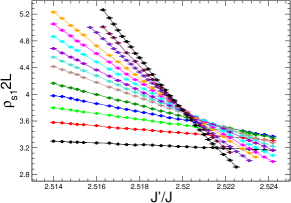
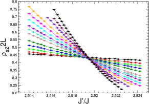
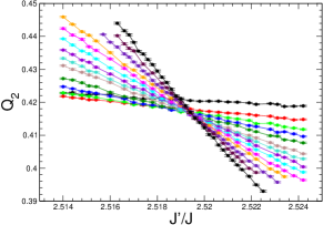
Figure 2: Monte Carlo data of $\rho_{s1}2L$ (top), $\rho_{s2}2L$ (middle), and $Q_{2}$ (bottom).

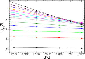
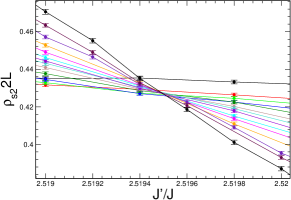
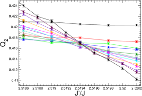
Figure 3: Crossing of $\rho_{s1}2L$ (top), $\rho_{s2}2L$ (middle), and $Q_{2}$ (bottom) for different $L$ near the transition.

Conclusions.— In this paper, we re-investigated the critical behavior at the phase transition induced by dimerization of the spin-1/2 Heisenberg model with a spatially staggered anisotropy. Unlike the scenario suggested in Wenzel08 that an unconventional universality class is observed, we conclude that indeed this second order phase transition is well described by the $O(3)$ universality class. Our observation of $\rho_{s2}2L$ being a good observable for determining the critical exponent $\nu$ is crucial for reading this conclusion by confirming the $O(3)$ critical exponent for this phase transition with high precision. While we do observed a large correction to scaling for the observable $\rho_{s1}2L$ as proposed in Fritz11 , the data points of $\rho_{s2}2L$ show good scaling behavior. Specifically, with $\rho_{s2}2L$, we can easily reach a highly accurate numerical value for $\nu$ consistent with the theoretical predictions without taking the confluent correction into account in the fit. The large correction to scaling observed for $\rho_{s1}2L$ in principle should influence all observables. Hence the most reasonable explanation for the good scaling behavior of $\rho_{s2}2L$ shown here is that the prefactor $b$ in Eq. (4) for $\rho_{s2}2L$ is very small. As a result, we are able to determine the expected numerical value for $\nu$ using data of $\rho_{s2}2L$ with moderate lattice sizes. Still, a more rigorous theoretical study such as investigating whether there exists a symmetry that protects $\rho_{s2}2L$ from being affected by the large correction to scaling as suggested in Fritz11 will be an interesting topic to explore. For example, in Fritz11 it is argued that the enhanced correction to scaling observed for this phase transition might be due to a cubic irrelevant term which contains one-derivative in the 1-direction. The first thing one would like to understand is whether the feature of this irrelevant term, namely it contains one-derivative in the 1-direction, will lead to our observation that the large correction to scaling has little impact on $\rho_{s2}2L$. In summary, here we present convincing numerical evidence to support that the phase transition considered in this study is well described by the $O(3)$ universality class prediction, at least for the critical exponent $\nu$ which is investigated in detail in this study. Finally, whether the good scaling of $\rho_{s2}2L$ observed here is a coincidence or is generally applicable for quantum Heisenberg models with a similar spatially anisotropic pattern, remains an interesting topic for further investigation. Acknowledgements.— We thank B. Smigielski for correcting the manuscript for us. Useful discussions with S. Wessel, M. Vojta, and U.-J. Wiese is acknowledged. Part of the simulations in this study were based on the loop algorithms available in ALPS library Troyer08 . This work is partially supported by NSC (Grant No. NSC 99-2112-M003-015-MY3) and NCTS (North) of R. O. C..

References

- (1) S. Wenzel, L. Bogacz, and W. Janke, Phys. Rev. Lett. 101, 127202 (2008).
- (2) L. Fritz et al., Phys. Rev. B 83, 174416 (2011)
- (3) B. B. Beard and U.-J. Wiese, Phys. Rev. Lett. 77 (1996) 5130.
- (4) A. W. Sandvik, Phys. Rev. B 56, 11678 (1997).
- (5) A. W. Sandvik, Phys. Rev. Lett. 83, 3069 (1999).
- (6) Y. J. Kim and R. Birgeneau, Phys. Rev. B 62, 6378 (2000).
- (7) L. Wang, K. S. D. Beach, and A. W. Sandvik, Phys. Rev. B 73, 014431 (2006).
- (8) F.-J. Jiang, F. Kämpfer, M. Nyfeler, and W.-J. Wiese, Phys. Rev. B 78, 214406 (2008).
- (9) S. Wenzel and W. Janke, Phys. Rev. B 79, 014410 (2009).
- (10) F.-J. Jiang, Phys. Rev. B 83, 024419 (2011).
- (11) F.-J. Jiang and U.-J. Wiese, Phys. Rev. B 83, 155120 (2011).
- (12) T. Pardini, R. R. P. Singh, A. Katanin and O. P. Sushkov, Phys. Rev. B 78, 024439 (2008).
- (13) F.-J. Jiang, F. Kämpfer, and M. Nyfeler, Phys. Rev. B 80, 033104 (2009).
- (14) M. Campostrini, M. Hasenbusch, A. Pelissetto, P. Rossi, and E. Vicari, Phys. Rev. B 65, 144520 (2002).
- (15) F.-J. Jiang and U. Gerber, J. Stat. Mech. P09016 (2009).
- (16) F.-J. Jiang, arXiv:0911.4721; arXiv:1010.6267.
- (17) A. F. Albuquerque et. al, Journal of Magnetism and Magnetic Material 310, 1187 (2007).