Outflow, Infall and Protostars in the Star Forming Core W3-SE

Abstract

We report new results on outflow and infall in the star forming cores W3-SE SMA-1 and SMA-2 based on analysis of $\sim$2.5$\arcsec$ resolution observations of the molecular lines HCN(3-2), HCO⁺(3-2), N₂H⁺(3-2) and CH₃OH(5_2,3-4_1,3) with the Submillimeter Array. A high-velocity bipolar outflow originating from the proto-stellar core SMA-1 was observed in the HCN(3-2) line, with a projected outflow axis in position angle 48$\arcdeg$. The detection of the outflow is confirmed from other molecular lines. An inverse P-Cygni profile in the HCN(3-2) line toward SMA-1 suggests that at least one of the double cores accretes matters from the molecular core. A filamentary structure in the molecular gas surrounds SMA-1 and SMA-2. Based on the SMA observations, our analysis suggests that the double pre-stellar cores SMA-1 and SMA-2 result from fragmentation in the collapsing massive molecular core W3-SE, and it is likely that they are forming intermediate to high-mass stars which will be new members of a star cluster in the W3-SE region.

1. Introduction

One of the key questions in the study of star formation is how protostars accrete material from their parent molecular clouds. Accretion around protostars with intermediate and high mass is not well understood due to lack of high-resolution observations. Observation of infall is needed to provide direct evidence for accretion. Low resolution observations of a blue-dominated double-peaked spectral profile as expected from a model of self-absorption in infalling gas clumps (NGC 1333-IRAS 2 as an example; see Ward-Thompson et al., 1996; Ward-Thompson & Buckley, 2001; Jorgensen et al., 2004a; Peretto et al., 2006) do not unambiguously identify infall because massive cores usually contain bipolar outflows, disk rotation and multiple sub-cores in addition to gas infall. Complex dynamical processes can produce characteristics similar to those expected from the self-absorption model of a molecular core with infall. It is crucial to carry out high-angular and spectral resolution observations along with comprehensive modeling of the dynamical processes involved in a massive star forming region.

There is growing evidence that massive stars form in groups, but accretion modeling has been for material concentrated in monolithic cores (McKee & Ostriker, 2007). The formation of binary and multiple stellar systems, especially those with two comparable-mass protostars and a large separation, is poorly understood (McKee & Ostriker, 2007). Detailed high-resolution observations of a binary/multiple proto-stellar system will provide valuable data for understanding accretion and outflow from each of the sub-cores in the system.

W3-SE is a dense molecular core located SE of the well-known massive star formation region W3-Main. We adopted a distance of $D$ = 2 kpc for W3-SE (Blitz et al., 1982; Xu et al., 2006). The spectral energy distribution (SED), along with a double continuum core revealed in our previous paper (Zhu et al., 2010) suggests that a total mass 65 M_☉ for the W3-SE core over a scale of 10$\arcsec$ is mainly composed of two proto-stellar cores of comparable masses, which are separated by 3.5$\arcsec$ or 7000 AU as revealed in the continuum observations with the Submillimeter Array (SMA). Observations of HCO⁺(1-0) using the CARMA telescope at 6$\arcsec$ resolution show that outflows appear to dominate the observed spectra although infall might also contribute to the spectrum toward the main molecular core which coincides with the double cores. Spectral-line observations with higher angular resolution are necessary to separate the contributions of infall and outflow from the double cores in W3-SE and to investigate the possibility of a protobinary system.

In this paper, we present results of analysis of spectral-line data observed with the SMA at $\sim$2.5$\arcsec$ resolution. Section 2 describes the observations and data reductions. Section 3 shows the results on the basis of our analysis of the molecular line data including HCN(3-2), HCO⁺(3-2), N₂H⁺(3-2) and CH₃OH(5_2,3-4_1,3). In Section 4, we present an interpretation of the observations in the context of outflow and infall. Section 5 gives a summary and conclusions.

2. Observations

The observations toward W3-SE consist of two tracks obtained at $\lambda$ 1.1 mm using the SMA in the compact configuration with an angular resolution of $\sim$2.5$\arcsec$ in 2008 October 27th and December 20th. The observations were centered at R.A.(J2000) = 02^h25^m54^s.50, DEC(J2000) = 62$\arcdeg$04$\arcmin$11$\arcsec$.0, which is used as the reference position in the following analysis. The LO frequency ($\nu_{\rm LO}$) for the 2008 October track was tuned to 271.7 GHz and $\nu_{\rm LO}$ = 285.3 GHz for the other. The observations consist of a lower side band (LSB) and an upper side band (USB) separated by 10 GHz, with a bandwidth of 2 GHz for each sideband. The typical system temperatures (T_sys) are 180-200 K and 200-250 K for the observations in October and December, 2008, respectively.

Data reduction and imaging were carried out in MIRIAD (Sault et al., 1995) with specific implementations for SMA data reduction. The bandpass was calibrated using QSOs 3C454.3 for the lower-frequency track and 3C273 for the higher-frequency track. For both tracks the complex gains were calibrated using QSO 0244+624. The flux density scale was bootstrapped from Uranus using the SMA planet model. By combining the visibility data from both LSB and USB, the continuum images achieve rms noises of 1.5 mJy and 3.0 mJy for the data observed in 2008 October and December, respectively. Spectral line images were made by subtracting the continuum emission from each visibility data using the MIRIAD task UVLIN.

3. Results

3.1. HCN(3-2)

A transition of hydrogen cyanide, HCN(3-2) at $\nu_{0}$ = 265.886 GHz, was observed in the LSB of the 2008 October observations. Figure 1a presents the HCN(3-2) channel maps, showing multiple velocity components distributed in the W3-SE core. In the velocity range between –39.3 and –38.0 km s^-1 a gap with no significant line emission signals is observed. The figure also shows compact HCN(3-2) components in the high-velocity channels ($<$ –46.7 km s^-1 and $>$ –30.5 km s^-1). Figure 2a shows the integrated line intensity map of HCN(3-2), suggesting the presence of three emission peaks from the HCN(3-2) line within the main molecular emission component A, as observed by CARMA at an angular resolution of 6$\arcsec$ (Zhu et al., 2010). We denote the three sub-components as A-NE, A-SW and A-SE, respectively. The HCN(3-2) line components A-NE and A-SW are located 2$\arcsec$ northeast and 4$\arcsec$ southwest of the proto-stellar core SMA-1 while the component A-SE nearly coincides with SMA-2. The integrated intensity of HCN(3-2) line emission in A-NE and A-SW is stronger than that from A-SE.

Figure 3 shows the spectra of the HCN(3-2) line in the core region of W3-SE with a boundary outlined by the square in Figure 2a. A significant absorption feature is shown in the core region at velocities in the range between –39.3 and –38.0 km s^-1. The component A-NE appears to be associated with a broad blue-shifted line wing, while A-SW shows a broad red-shifted line wing. The highly blue-shifted line wing associated with A-NE shows a maximum absolute radial velocity of 35 km s^-1 (above the 5 $\sigma$ cutoff), with respect to SMA-1. Here an LSR systemic velocity $V_{\rm sys}$ = –39.1 km s^-1 is used, which is determined from the peak velocity of the optically thin line CH₃OH(5_2,3-4_1,3). In the region of A-SW, the red-shifted line wing shows a maximum absolute radial velocity of 33 km s^-1 (above 5 $\sigma$) with respect to SMA-1. The velocity profile for both blue- and red-shifted broad line wings can be fitted to a power law ($\sim$$|V-V_{\rm sys}|$^-γ) with an index of $\gamma\approx 2.0$. The power-law distribution of molecular content as function of velocity observed is consistent with numerical models of bow-shock outflow (e.g., Downes & Ray, 1999; Lee et al., 2001).

In Figure 4a, we show the high-velocity gas in both the blue-shifted (–74.1 to –45.2 km s^-1) and red-shifted (–31.9 to –5.8 km s^-1) outflow lobes, located NE and SW of the proto-stellar core SMA-1 with separations of 2.2$\arcsec$ and 5.0$\arcsec$, respectively. The configuration of the emission from the high-velocity wings, along with the location of SMA-1 suggests a bipolar outflow originating from SMA-1, a possible energy source in the region. The major axis of the outflow is shown as a straight line connecting the two peaks of the blue- and red-shifted knots in Figure 4a, at P.A. = 48^∘. Although the location of SMA-1 appears to be offset from the outflow axis by $\sim$0.4$\arcsec$, about 5% of the distance between the two high-velocity knots, such an apparent offset could be due to the uncertainty ($\sim$0.2$\arcsec$) in the peak position of SMA-1 given by Gaussian fitting.

In summary, the high-velocity HCN(3-2) line emission from the two compact molecular components A-NE and A-SW appears to be excited by a high-velocity bipolar outflow originating from the proto-stellar core SMA-1.

3.2. HCO⁺(3-2)

The transition of HCO⁺(3-2) at 267.558 GHz was also included in the LSB of the observations at $\nu_{\rm LO}$ = 271.7 GHz. Figure 1b shows the channel maps of the HCO⁺(3-2) line. The overall distribution of HCO⁺ gas in velocity is consistent with that of HCO⁺(1-0) observed with CARMA (Zhu et al., 2010) and similar to that of HCN(3-2) in the SMA observations, showing multiple emission peaks at various velocities and a gap in the velocity range between –38.9 and –37.9 km s^-1.

However, not all of the emission peaks observed in HCO⁺(3-2) coincide with those in HCN(3-2). In the integrated intensity map of HCO⁺(3-2) in Figure 2b, the emission peak A-NE observed in HCN(3-2) appears to be embedded in the surrounding emission, and A-SW in HCO⁺(3-2) is not as prominent as it is in HCN(3-2). Instead, strong emission in HCO⁺(3-2) appears to be concentrated in a bright ridge 0.5$\arcsec$ northeast of the line connecting the double proto-stellar cores SMA-1 and SMA-2. Outside the main core A, the molecular sub-core B and the molecular tail C are also present, in good agreement with the image of HCO⁺(1-0) observed with CARMA. In comparison with the HCN(3-2) image, the HCO⁺(3-2) line appears to trace a more extended envelope around the double proto-stellar cores.

As Figure 5 shows, the observed HCO⁺(3-2) spectra are also found with broad line wings at the position of SMA-1 and its adjacent region, although the line wings in HCO⁺(3-2) are not as significant and broad as that in HCN(3-2) spectra. The integrated intensity map for the blue- and red-shifted line wings is shown in Figure 6a. The velocity ranges for the integrations are (–57.9, –45.3) km s^-1 and (–31.8, -18.8) km s^-1, with the same lower velocity limits as that for HCN(3-2). In Figure 6a, the compact blue- and red-shifted lobes are offset from SMA-1 similar to the case of HCN(3-2), although they are closer to SMA-1 (1.3$\arcsec$ for the blue lobe, and 3.4$\arcsec$ for red lobe) than the lobes in HCN(3-2). This could be explained if HCN(3-2) emission is excited close to bow shocks, while HCO⁺(3-2) traces colder and more extended gas which is farther from bow shocks. Another possible reason is that the emission of the high-velocity outflow lobes might be blended by the HCO⁺(3-2) emission from a large-scale outflow (Zhu et al., 2010) and other dynamical components associated with SMA-2. Indeed, in Figure 6a a red-shifted HCO⁺(3-2) component is found close to SMA-2 at high velocity. The same component is also marginally detected in HCN(3-2) (see Figure 4a), and it might be an outflow component associated with SMA-2.

The low-velocity line wings of the HCO⁺(3-2) spectra were also integrated with the velocity ranges (–44.9, –41.7) km s^-1 and (–36.3, –32.3) km s^-1 for blue and red lobes, respectively. The velocity ranges have similar lower velocity limits as the ones used in previous HCO⁺(1-0) study (Zhu et al., 2010). As Figure 6b shows, the distribution of blue- and red-shifted low-velocity HCO⁺(3-2) gas is consistent with the results of HCO⁺(1-0), implying a possible large-scale outflow in a NW-SE direction.

3.3. N₂H⁺(3-2)

A transition of protonated nitrogen, N₂H⁺(3-2) at $\nu_{0}$ = 279.512 GHz was included in the LSB of the 2008 December observations. Figure 2c shows the integrated intensity map of N₂H⁺(3-2), indicating multiple N₂H⁺(3-2) emission clumps which form a curved filamentary emission region. Among the numerous N₂H⁺(3-2) emission peaks, the two strongest emission peaks appear to be located near SMA-1 and SMA-2 with a displacement of $\sim$0.5$\arcsec$ from the continuum peaks, suggesting that a close relationship between the dense molecular gas and the proto-stellar cores.

The bright N₂H⁺(3-2) emission region is located SW of the double continuum cores, opposite to the locations of the bright emission ridge of HCO⁺(3-2). Emission at the locations of SMA-1 and SMA-2 might be influenced by excitation or chemical conditions. The primary formation routes for both HCO⁺ and N₂H⁺ involve reactions with H${}_{3}^{+}$. For a higher CO abundance, the main formation route is the reaction between CO and H${}_{3}^{+}$ in forming HCO⁺. While when the CO abundance gets low enough, the reaction between H${}_{3}^{+}$ and N₂ in forming N₂H⁺ becomes the main mechanism for the removal of H${}_{3}^{+}$ (Jorgensen et al., 2004b). In addition, as CO returns to the gas phase from a freezing-out phase, destruction of N₂H⁺ through reactions with CO becomes the dominant removal mechanism for N₂H⁺. The possible anti-correlation of the bright emission regions between N₂H⁺(3-2) and HCO⁺(3-2) near the proto-stellar cores might reflect a gradient of the CO abundance across the W3-SE core.

The line profiles of N₂H⁺(3-2) spectra towards SMA-1 and SMA-2 are shown in Figure 7. We noticed the skewness of the line profiles, i.e., at the position of SMA-1, the N₂H⁺(3-2) spectrum mimics a “blue-profile”, while toward SMA-2 N₂H⁺(3-2) is like a “red-profile”. The main hyperfine structures of the transition $J$=3-2 for N₂H⁺ spread over a frequency range of only a few 100 kHz (100 kHz $\sim$ 0.1 km s^-1), while the velocity difference between the two emission peaks of the N₂H⁺(3-2) spectrum toward SMA-1 is $\sim$5.0 km s^-1. Therefore, it is unlikely that the observed skewness in the N₂H⁺(3-2) line profile is due to hyperfine structure.

In order to model the overall kinematics of the molecular filament in the region, a centroid velocity map of N₂H⁺(3-2) was made (see Figure 8a) by calculating $v_{\rm cen}=\int{vI_{v}}{\rm d}v/\int{I_{v}}{\rm d}v$ at each position. Here $v_{\rm cen}$ is the centroid velocity (intensity-weighted mean velocity), and $I_{v}$ is the intensity of the spectrum at a given velocity $v$. In general, the distribution of the centroid velocity shows a gradient of 30$\pm$10 km s^-1 pc^-1 over a spatial scale of $\sim$20$\arcsec$, i.e., the gas in NW is red-shifted while that in SE is blue-shifted. This velocity structure appears to be similar to the large-scale velocity structure traced by HCO⁺(1-0) that is believed to be a result of outflow (Zhu et al., 2010).

3.4. CH₃OH(5_2,3-4_1,3)

The methanol transition CH₃OH(5_2,3-4_1,3) at $\nu_{0}=266.838$ GHz was observed in the LSB in the October 2008 observations. Figure 2d shows the integrated intensity map of this transition. The two main CH₃OH(5_2,3-4_1,3) emission peaks coincide with the two proto-stellar cores SMA-1 and SMA-2 within the uncertainty in position ($\sim$0.2$\arcsec$), indicating that this line traces the densest part of the cores and could be used to determine the systemic velocity. The methanol emission appears to mainly arise from the two proto-stellar cores as well as the high-velocity outflow from SMA-1. In addition, in region B, a weak signal of CH₃OH(5_2,3-4_1,3) is detected at a 3$\sigma$ level. No significant emission from CH₃OH(5_2,3-4_1,3) was detected towards region C. The distribution of the centroid velocity in CH₃OH emission (Figure 8b) has no significant velocity gradients, although at the northwest boundary and the position of A-SW the centroid velocity is slightly red-shifted.

3.5. Comparison of Molecular Line Spectra towards SMA-1 and SMA-2

Figure 7 shows the spectra from the peak positions of SMA-1 and SMA-2 in the lines of HCN(3-2), HCO⁺(3-2), N₂H⁺(3-2) and CH₃OH(5_2,3-4_1,3), respectively. In general, double-peak profiles appear to characterize the optically thick lines toward both cores from different molecules. For a given molecular line, the double-peaked profile of SMA-1 is dominated by the blue-shifted feature, whereas in SMA-2, the red-shifted peak is stronger than the blue-shifted one. For a given core, the separation between the peaks of the double-peak line profile appears to vary. For example, in the case of SMA-1, the velocity separations between the two spectral peaks vary significantly from 7.6 km s^-1 for the HCN(3-2) line to 4.0 km s^-1 for both the HCO⁺(3-2) and N₂H⁺(3-2) lines, suggesting that different molecular lines may trace different dynamic processes or chemistry in a proto-stellar core. For the HCN(3-2) line from SMA-1, the large velocity separation of 7.6 km s^-1 between the double emission peaks is probably due to the high-velocity bipolar outflow because the HCN(3-2) line is the best tracer of the shocked and compressed medium among the four observed molecular lines shown in this paper.

In contrast to the double spectral peaks observed in HCN(3-2) and HCO⁺(3-2), the hot molecular line CH₃OH(5_2,3-4_1,3) shows a single-peaked profile toward both the proto-stellar cores. Gaussian fits to the spectra show that CH₃OH(5_2,3-4_1,3) are peaked at –39.1$\pm$0.1 km s^-1 for both SMA-1 and SMA-2. We use this as the systemic velocity in this paper, i.e. $V_{\rm sys}$ = –39.1 km s^-1. The apparent peak velocities of the spectra have a difference of $\sim$0.4 km s^-1, equivalent to the width of one channel. Figure 8b also suggests a difference $\sim$0.5 km s^-1 between the centroid velocities of CH₃OH(5_2,3-4_1,3) toward the two cores. However, this inconsistency could be due to the slightly asymmetric CH₃OH(5_2,3-4_1,3) line profile toward SMA-2 and contamination from the complex kinematics in W3-SE region (e.g. the outflow from SMA-1). Thus, we conclude that there is no significant difference between the radial velocities of CH₃OH(5_2,3-4_1,3) from SMA-1 and SMA-2.

An emission bump at –40.2 km s^-1 is present in the spectral dip between the double HCN(3-2) emission peaks toward SMA-1 (see left-top panel in Figure 7). The velocity of the emission bump appears to correspond to the velocity of the blue-shifted peak in both the HCO⁺(3-2) and N₂H⁺(3-2) lines, which is blue-shifted with respect to the systemic velocity. In addition, the red-shifted dip between the two main emission peaks appears to be an absorption feature and the intensity becomes negative ($\sim$ 5 $\sigma$) at –37.6 km s^-1. We will discuss these spectral features in Section 4.2.1.

4. Discussion

4.1. High-velocity Bow-shock Outflow in HCN(3-2)

Two possible mechanisms for accelerating molecular gas in outflows from proto-stellar cores are stellar winds and highly collimated jets (e.g. Downes & Ray, 1999). The broad velocity distribution with a power law in both blue- and red-shifted HCN(3-2) line wings and the morphology of the high-velocity HCN(3-2) lobes suggests that high-velocity HCN(3-2) emission is excited at jet-driven bow shocks. An outflow model with jet-driven bow shocks has been studied both analytically and numerically (e.g. Downes & Ray, 1999; Lee et al., 2000). In the case of W3-SE, a P-V diagram along the major axis of the bipolar outflow observed in the HCN(3-2) line (Figure 9) shows similar characteristics to that predicted from the bow-shock model. The broad blue- and red-shifted velocity gas components show significant offsets of 2.2$\pm$0.2$\arcsec$ and 5.0$\pm$0.2$\arcsec$ from SMA-1, providing evidence that the high velocity HCN(3-2) gas is indeed excited and accelerated at the bow-shocked sites outside of the proto-stellar core SMA-1.

To characterize the observed high-velocity outflow, we adopted a simple model of bow-shock outflow (Downes & Ray, 1999), in which the geometry and velocity of the molecular gas along the bow-shock surface can be worked out in analytical forms. Using the model illustrated in Figure 10, a cylindrical symmetric outflow radius ($r$) and major axis ($z$) plane are used following Downes & Ray (1999). We derived equations for the four boundaries that outline the observed P-V diagram (see Appendix). A power-law (${\displaystyle z\sim|r|^{s}}$) with an index $s=2$ for the locus of the bow-shock surface is assumed in fitting the model to the observed P-V diagram of the bipolar outflow from SMA-1 as discussed below. The systemic velocity, V_sys = –39.1 km s^-1, and the projected angular offsets of the blue- and red-shifted bow-shock tips ($a_{B}\approx 2.2\arcsec$ and $a_{R}\approx 5.0\arcsec$) from the outflow origin have been determined directly from the peak velocity of the hot molecular line CH₃OH(5_2,3-4_1,3) (Figure 7) and the HCN(3-2) outflow map (Figure 4a), respectively. The remaining two free parameters $\alpha$ (inclination angle) and $v$ (the velocity of bow-shock with respect to the origin of the outflow) were assumed to have equal values for the blue- and red-shifted lobes, and they can be determined by comparing the observed P-V diagram and the curve from the bow-shocked outflow model. Figure 9 shows the observed P-V diagram in contours and the curves derived from the bow-shock outflow model in thick lines. A shock velocity $v$ = 40 km s^-1 and three different inclination angles $\alpha$ = 55$\arcdeg$, 70$\arcdeg$, and 85$\arcdeg$ were used to generate the curves. It appears that the model with $v$ = 40$\pm$10 km s^-1 and $\alpha$ = 70$\pm$5$\arcdeg$ best fits the overall line wings of the P-V diagram. To estimate the uncertainty (1 $\sigma$) in the values of $v$ and $\alpha$, we added small offset to cause the derived model curve to offset by one contour interval of the P-V diagram (3 $\sigma$). The inferred shock velocity of the bipolar outflow implies a dynamic age of 3$\times$10³ yr for the the proto-stellar core SMA-1, which is an order of magnitude younger than that inferred for the possible large-scale molecular outflow in the region (Zhu et al., 2010), indicating that the source(s) embedded in SMA-1 is probably very young. On the other hand, SMA-1 is known to be associated with mid-IR source (Zhu et al., 2010) which implies the existence of heating source in SMA-1. We offer two possible explanations, i.e. the protostar in SMA-1 has a large mass and evolves more rapid than classic low-mass stars, or there are multiple YSOs embedded in SMA-1 and the compact outflow and the mid-IR source are actually associated with different YSOs.

4.2. Infalling Gas toward SMA-1

4.2.1 Possible Infall Signature

The blue-dominated double-peaked profile of the HCO⁺(1-0) spectrum toward core A observed using CARMA at 6$\arcsec$ resolution was fitted using a model with both outflow and infall components (Zhu et al., 2010). The fit suggests that outflow significantly contributes to the spectral profile, particularly in the high-velocity wings. The high-velocity outflow lobes from SMA-1 are separated from the proto-stellar core in the SMA HCN(3-2) observations at (2.5$\arcsec$$\times$2.3$\arcsec$) resolution. Contamination from the high-velocity outflow in the spectra toward the cores has been reduced to a level where an inverse P-Cygni profile, a signature of infall, would become noticeable if it exists.

The HCN(3-2) spectra (Figure 3), show blue-shifted emission at –40.2 km s^-1 toward SMA-1 and the adjacent region, with a sharp dip in the emission at –37.6 km s^-1. The systemic velocity of –39.1 km s^-1 lies between the two spectral features. The complexity of the HCN(3-2) line profile toward SMA-1 might be due to a superimposition of an inverse P-Cygni profile and a broader double-peaked profile from the high-velocity bipolar outflow. Such an explanation is consistent with the hypothesis that gas is infalling to SMA-1 (Zhu et al., 2010).

Figure 7 shows that toward SMA-1 the intensity of the HCN(3-2) dip at –37.6 km s^-1 becomes negative. The spectral dip could be partially caused by unsampled short-spacings. However, in our observations the shortest projected baseline is 5.4 k$\lambda$, corresponding to a spatial scale of $\sim$38$\arcsec$. Thus for the spectrum toward SMA-1 with a beam size (2$\arcsec$.5$\times$2$\arcsec$.3), flux missing should not be a severe problem. We can roughly estimate the short spacing effect using the previous study of CARMA data. For the HCO⁺(1-0) spectra at the peak position, the flux density of the spectral dip was raised to 0.5 Jy beam^-1 from 0.0 Jy beam^-1 after combining with single-dish data. Assuming that the missing flux density of 0.5 Jy beam^-1 is evenly distributed in a structure on a scale of the CARMA beam (6$\arcsec$.3$\times$5$\arcsec$.7), and toward SMA-1 the flux density of HCN(3-2) is the same as HCO⁺(1-0), the missing flux in HCN(3-2) at the velocity of the dip is less than 0.1 Jy within the SMA beam. On the other hand, the intensity of HCN(3-2) towards SMA-1 is $\sim$–1 K ($\sim$–0.4 Jy beam^-1) at the spectral dip. Therefore, in the case of W3-SE the missing flux caused by unsampled short spacings has only a small influence in the core region on a scale of the beam size, and the observed negative intensity for the HCN(3-2) spectral dip is likely to be real.

If the emission bump is explained as an inverse P-Cygni feature, the infalling gas associated with SMA-1 appears to be confined to a region $\sim$6$\arcsec$ ($\sim$12000 AU) with velocities in a range of (–40 to –38 km s^-1) that is close to the systemic velocity of the proto-stellar core. We made an integrated intensity map of this emission in a velocity range from –40.0 to –39.5 km s^-1 (Figure 4b). This image clearly shows that the HCN(3-2) feature is associated with SMA-1, thus SMA-1 is likely to be the gravitational center. Weak HCN(3-2) emission to the SE of SMA-1 at a similar radial velocity, could blend with the observed HCN(3-2) spectra from SMA-1.

4.2.2 A General Model Including Both Infall and Outflow

In order to separate the possible inverse P-Cygni (infall) feature from the outflow, we adopted a characteristic model with a continuum core in the middle comprised by two layers of infalling gas and two layers of outflowing gas located outside of the infall core, which is hereafter referred to as a four-layer model (Myers et al., 1996; Di Francesco et al., 2001; Attard et al., 2009). The schematic configuration of the model is illustrated in the Figure 4 of Attard et al. (2009).

In the following discussion, the subscripts $f$, $r$, $B$, $R$ and $c$ are used to represent the front infall layer, rear infall layer, blue-shifted outflow layer, red-shifted outflow layer and the continuum core, respectively. On the assumption of homogeneous and isothermal layers of gas, the line intensity or brightness temperature from the “four-layer complex” can be solved from the radiative transfer equation for given excitation temperatures $T_{f}$ and $T_{r}$ of the front and rear layers of infall, $T_{\rm out}$ of both the outflow layers, and $T_{c}$ of the continuum emission. The line brightness temperature, after subtracting the continuum in which the contribution from the cosmic background radiation is negligible, can be expressed as:

$$\Delta T_{L} = J(T_{f})\Bigg{[}\left(1-\frac{J(T_{c})f_{c}(1-e^{-\tau_{c}})}{J(T_{f})}\right)(1-e^{-\tau_{f}})+$$ (1)

$$\frac{J(T_{r})}{J(T_{f})}(1-e^{-\tau_{r}})e^{-\tau_{f}-\tau_{c}}\Bigg{]}e^{-\tau_{B}}+$$

$$J(T_{\rm out})\Bigg{[}\left(1-\frac{J(T_{c})f_{c}(1-e^{-\tau_{c}})}{J(T_{\rm out})}\right)(1-e^{-\tau_{B}})+$$

$$(1-e^{-\tau_{R}})e^{-\tau_{B}-\tau_{f}-\tau_{c}-\tau_{r}}\Bigg{]},$$

where ${\displaystyle J(T)=\frac{h\nu}{k}\left(e^{h\nu/kT}-1\right)^{-1}}$ is a radiation temperature of each layer and $f_{\rm c}$ is the beam filling factor for the continuum emission. Equation 1 shows that, in the four-layer model, the resultant line-profile can be expressed as two separated terms. The term in the first bracket on the right side of Equation 1 describes the line profile of the in-falling gas, corresponding to an inverse P-Cygni profile in the case of $J(T_{c})f_{c}\tau_{c}$$>$$J(T_{f})$. The infall line profile is attenuated by the absorption in the blue-shifted outflow ($e^{-\tau_{B}}$). The term in the second bracket corresponds to the line profile from the bipolar outflow showing a classical P-Cygni profile if $J(T_{c})f_{c}\tau_{c}$$>$$J(T_{\rm out})$ or a red-dominated double-peaked profile if $J(T_{c})f_{c}\tau_{c}$$<$$J(T_{\rm out})f_{\rm out}$. The emission from the red-shifted outflow layer is attenuated by the absorbing gas in both the infall layers and the blue-shifted outflow as well as the continuum dust ($e^{-\tau_{f}-\tau_{r}-\tau_{B}-\tau_{c}}$).

Each of the optical depths in the four layers can be modeled using a Gaussian function with a mean velocity and a velocity dispersion for infall ($V_{\rm in}$, $\sigma_{\rm in}$) and outflow ($V_{\rm out}$, $\sigma_{\rm out}$) assuming the systemic velocity of $V_{\rm sys}$. Therefore, a total of fourteen parameters, namely, the five kinematic parameters ($V_{\rm in}$, $V_{\rm out}$, $\sigma_{\rm in}$, $\sigma_{\rm out}$ and $V_{\rm sys}$) along with four excitation temperatures ($T_{f}$, $T_{r}$, $T_{\rm out}$ and $T_{c}$) and five optical depths ($\tau_{f}$, $\tau_{r}$, $\tau_{B}$, $\tau_{R}$ and $f_{c}$$\tau_{c}$) are required to characterize the physical conditions of the gas in each layer.

4.2.3 Fitting the HCN(3-2) Spectra

We made a tentative fitting to the observed HCN(3-2) spectra with the model described by Equation 1. In the case of W3-SE, the quantities for the continuum emission ($T_{c}$ = 40 K and $\tau_{c}$ = 0.5) can be determined from the SED as discussed by Zhu et al. (2010) assuming that the ratio of 2:1 in dust content between SMA-1 and SMA-2 is proportional to the ratio of the total between the two sources. Therefore, thirteen free parameters are needed.

In order to fit the four-layer model to the observed HCN(3-2) line profiles, we first assumed the two outflow layers are optically thin at low velocities and fit the low-velocity part (from –43.5 to –34.1 km s^-1), or the assumed infall part, with the least-square approach. The high-velocity parts of the blue wings ($<$ –43.5 km s^-1) and red ($>$ –34.1 km s^-1) of HCN(3-2) are related to the bow-shock, and could not be fitted with Equation 1. Therefore, they are fitted separately with a power-law profile (${\displaystyle\propto~{}|V-V_{\rm sys}|^{-\gamma}}$). The maximum intensities of the power-law line wings are set to be at –43.5 and –34.1 km s^-1 for blue and red wings, respectively, and the values are obtained from fitting the low-velocity line profile with Equation 1.

The best fitting results are shown in Figure 11a, which gives an infall velocity 0.9 km s^-1. The derived excitation temperatures are 6${}^{+1}_{-2}$ and 11$\pm 3$ K for the front and rear layers, respectively. The best fits for the thirteen free parameters in the final stage was adjusted by eye to achieve a minimum residual. The errors (1$\sigma$) were assessed by adding an offset (3$\sigma$) to a best-fitted quantity with other parameters fixed, to increase the offset of the best-fitted curve from the observed profile (or a factor of 3 increase in the residual). The higher excitation temperature for the rear layer might suggest the presence of a temperature gradient in radius (temperature increases as it gets close to the protostar). Thus, an observer receives emission from colder part in the front and warmer part in rear layers, considering the optical-depth effect. On the other hand, the excitation temperature of the in-falling gas is also constrained by the observed brightness temperature in the presence of an inverse P-Cygni profile. As both angular and spectral resolution improve, observations with interferometer arrays at millimeter and sub-millimeter wavelengths will place more meaningful constraints on the in-falling gas in proto-stellar cores. For the bipolar outflow in SMA-1, the gas components in both the blue- and red-shifted outflows are optically thin ($\tau_{\rm out}\sim$0.1) with excitation temperatures of $\sim$75 K, which are much higher than the beam-averaged peak brightness temperature ($\sim$8 K) of HCN(3-2). As for the high-velocity parts of the spectrum, the power-law index $\gamma$ for the blue and red lobes of the outflow are 2.0 and 2.5, respectively. The difference of the two values could be due to a slight difference in the directions of the ejected blue- and red-shifted high-velocity gas components.

Fitting the four-layer model to the spectral profile of SMA-2 suggests that a bipolar outflow might also be present in this proto-stellar core (see Figure 11b). In comparison, the expected outflow from SMA-2 has a similar optical depth and excitation temperature to those derived from SMA-1 but it appears at an earlier stage. The observed line profile in the low-velocity range appears to be dominated by outflow emission and no obvious infall signatures are present toward SMA-2. SMA-2 is different from SMA-1 since it has no obviously associated mid-IR point sources. The relative extended mid-IR emission in the adjacent of SMA-2 might be due to the external heating from the formed star in the W3-SE region.

We compared these fits with HCN(3-2) data with previous fits to CARMA HCO⁺(1-0) data of lower angular resolution ($\sim$6$\arcsec$) using a similar four-layer model (Zhu et al., 2010). All the parameters from the HCN(3-2) fits (see the caption of Figure 11) are consistent with the previous HCO⁺(1-0) fits, especially the infall velocity (0.9 km s^-1). Different from the HCO⁺(1-0) fits, the HCN(3-2) suggests an inverse P-Cygni profile instead of a blue profile, which could be due to the larger contribution from the high-velocity outflow in HCN(3-2) and the significant improvement of angular resolution.

We found it is implausible to obtain consistent fits with Equation 1 for the entire W3-SE region, and the fitted values of $\tau_{f}$, $\tau_{r}$, $T_{f}$ and $T_{r}$ change dramatically at difference positions. It could partially due to the contaminations from other components, such as potential further multiplicity, the possible large-scale outflow, and the possible high-velocity outflow associated with SMA-2. A more essential cause could be the over-simplified assumptions of the model itself, which assumes complete overlaps of the layers along the light of sight. A more detailed model should consider the two dimensional geometry of the W3-SE region and include the influences of the core SMA-2, the additional HCN(3-2) blue-shifted component and other possible components. Although due to the limit of the model we can only qualitatively analyze most of the fitted physical parameters, an exception is the infall velocity ($V_{\rm in}$). It can be consistently fitted for the spectra from different positions; its value is always between 0.8 and 0.9 km s^-1 and it is not sensitive to other fitted parameters. Actually it is also consistent with the velocity difference between the HCN(3-2) emission “bump” and the assumed systemic velocity.

Although fitting the HCN(3-2) spectrum towards SMA-1 is a tentative exercise, the fitting demonstrates a possible explanation: a complex including both high-velocity wings and an inverse P-Cygini profile, for the observed HCN(3-2) line profile toward SMA-1 region. A multiple-outflow model for the observed profile toward SMA-1 can be ruled out since no absorptions against the continuum are expected from the outflow gas with an excitation temperature of $\sim 75$ K, which is an order of magnitude larger than the brightness temperature of the continuum emission ($8$ K) at the observing wavelength. However, an alternative model with multiple outflows together with a cold envelope might fit the observed spectral profile. High-resolution observations of dense molecular lines at higher frequencies and a more sophisticated model are needed to unambiguously determine the nature of the observed profile towards SMA-1.

4.3. The Nature of the Double Cores in W3-SE

The W3-SE dust core is associated with a total mass of 65$\pm$10 M_☉ in a 15$\arcsec$ region, and is characterized by two continuum emission sources SMA-1 and SMA-2 with a projected angular separation 3.5$\arcsec$ or 7000 AU. SMA-1 and SMA-2 contribute 1/2 and 1/4 of the total flux density in 1.1-mm continuum, respectively (Zhu et al., 2010). Assuming a uniform distribution for both dust temperature and dust-to-gas ratio over the entire W3-SE region, a mass of 32$\pm$5 M_☉ is inferred for SMA-1 and 16$\pm$2 M_☉ for SMA-2. In the vicinity of the double proto-stellar cores, at least three additional mid-infrared sources have been revealed by Spitzer, indicating that the double cores located within or near SMA-1 and SMA-2 might be a young cluster (Zhu et al., 2010). Both the SMA and CARMA observations of the molecular lines reveal a common filamentary envelope of molecular gas surrounding the two main proto-stellar cores, suggesting that SMA-1 and SMA-2 result from fragmentation of molecular gas in the same parent cloud.

The dust temperature of the W3-SE core region (covering SMA-1 and SMA-2) $\sim$40 K, indicating that the gas in the core region is likely to be heated by both internal and external energy sources. Indeed, a group of mid-IR sources are located east of SMA-1 and SMA-2, and mid-IR emission is also detected in SMA-1 (Zhu et al., 2010). The high temperature implies a relatively large Jeans mass. Assuming a mass of 65 M_☉ evenly distributed in a 15$\arcsec$ region ($\sim$0.15 pc), a Jeans mass could be estimated by

$$M_{\rm J}=1.2\times 10^{5}(\frac{T}{100~{}K})^{3/2}(\frac{\rho}{10^{-24}~{}{\rm g}~{}{\rm cm}^{-3}})^{-1/2}{\mu}^{-3/2}~{}M_{\sun}$$

(Lang, 1998), where $\mu$ is the mean molecular weight and assumed to be 2.35. The inferred Jeans mass is $\sim$7 M_☉, far less than the derived masses of SMA-1 and SMA-2.

The observed infall signature might be due to global infall and/or inflow toward SMA-1. Although the spectra of HCN(3-2) and HCO⁺(3-2) appear to be dominated by outflow, they still present significant red-shifted absorption (see Figure 7). The HCO⁺(1-0) spectrum toward the W3-SE core, which covers both SMA-1 and SMA-2, also shows the infall signature (Zhu et al., 2010). A global infall in W3-SE is likely to occur as the inferred Jeans mass is far less than the total mass of the W3-SE molecular core. However, both the spectral map (Figure 3) and the integrated intensity map (Figure 4b) show that the possible inverse P-Cygni profile in HCN(3-2) is present toward SMA-1, the major one of the double cores in W3-SE.

SMA-1 and SMA-2 may result from fragmentation of a common parent molecular cloud. The mechanisms for binary formation have been discussed by Tohline (2002). The location of SMA-1 and SMA-2 within a common filament (Figure 2c) suggests that the two cores result from a prompt fragmentation mechanism (Tohline, 2002). Considering the projected separation, $d$ = 7000 AU (3.5$\arcsec$) for SMA-1 and SMA-2, and their total mass, $M_{\rm tot}\approx 50$ M_☉, they could be gravitationally bound if their actual separation is comparable to projected one. Assuming SMA-1 and SMA-2 rotate around their mass center with a distance $d$, the orbital period $\displaystyle P=(2\pi{d^{3}})^{1/2}\left(GM_{\rm tot}\right)^{-1/2}\approx 3\times 10^{4}$ yr and the relative velocity of the two cores $\sim$2.5 km s^-1. Although no significant difference in the radial velocities of the double cores is seen in our observations, this could be explained if the orbit is nearly face-on as implied by the large inclination angle ($\sim$70$\arcdeg$) of the high-velocity outflow in HCN(3-2) originating from SMA-1 (Section 4.1). The W3-SE proto-stellar system appears to be very young with an age $\sim 3\times$10³ yr inferred from the kinematic timescale of the outflow. This is an order magnitude smaller than the orbital period if the molecular core W3-SE is to form a protobinary system, indicating it is still an unrelaxed system. However, the possibility that SMA-1 and SMA-2 will relax to a gravitationally-bound binary system cannot be ruled out. Accretion could decrease the separation of the double cores and help the formation of a binary as suggested in the theory of dynamical hardening (Bonnell & Bate, 2005).

W3-SE can be compared with NGC 1333 IRAS 4, which was reported as a binary system consisting of two proto-stellar cores 4A (9.2 M_☉) and 4B (4.0 M_☉) with an angular separation $\sim$30$\arcsec$ ($\sim$9000 AU) at a distance of $\sim$300 pc (Sandell et al., 1991). In follow-up observations with higher-angular resolution, further multiplicities in both the sub-cores 4A and 4B have been revealed (e.g. Lay et al., 1995; Looney et al., 2000). Given the large masses for both SMA-1 and SMA-2 in W3-SE and the limited angular resolutions of the existing studies, SMA-1 and SMA-2 might turn out to be composed of multiple sub-cores in higher-resolution observations. The observed adjacent IR sources (Zhu et al., 2010) and multiple outflows also suggest further multiplicity in SMA-1 and SMA-2.

5. Summary

Following our previous study with continuum and spectral lines at low angular resolution, we made high-resolution observations of multiple molecular lines toward the double proto-stellar cores SMA-1 and SMA-2 in W3-SE. The two proto-stellar cores are located in a molecular filamentary structure which shows an active star-forming region in W3-SE. A high-velocity bipolar outflow originating from SMA-1 is seen in HCN(3-2), with confirmation from other molecular lines, which shows a star formation activity in W3-SE. The morphology and the velocity profile of the bipolar outflow fit a bow-shock outflow model. SMA-1 and SMA-2 appear to result from fragmentation of a collapsing massive molecular core. Global collapse and gas infall are suggested by red-shifted self-absorption observed in both HCN(3-2) and HCO⁺(3-2). An inverse P-Cygni feature observed in the HCN(3-2) line toward the proto-stellar core SMA-1 suggests that SMA-1 is the major accretion source in W3-SE. The double proto-stellar cores in W3-SE are ideal targets for further observations with higher angular and spectral resolution at (sub-)millimeter wavelengths in order to understand the formation of clusters with intermediate-mass stars.

Appendix A Bow-shock Model for Outflow

The bow-shock model (Downes & Ray, 1999) is one of the two popular models that provide mechanisms to accelerate molecular gas in an outflow. The observed features of the high-velocity bipolar outflow from SMA-1 appears to show the characteristics of a bow-shocked outflow as described in both numerical simulations and analytical models. In order to fit the P-V diagram from the observed HCN(3-2) outflow with the bow-shock model, we have worked out the formulas to outline the boundary of a P-V diagram from a bow-shock surface based on the analytical model of Downes & Ray (1999). In this model the bow-shock discontinuity is described as a rigid surface moving in the interstellar medium with a value of bulk velocity $v$. For instance, in a cylindrical coordinate system, the locus of the bow shock in a blue-shifted outflow lobe can be described as:

$$z=a-\mid{r}\mid^{s},~{}s{\geq}2,$$ (A1)

where $z$ is an axis along the direction of the bulk velocity of the bow-shock surface, $r$ is radius perpendicular to axis $z$, and $s$ is a power-law index to describe the curvature of the bow-shock surface (see Figure 10). In addition, the bow-shocked surface is treated as a rigid body. We made the further assumptions used in the following reduction. In the bow-shock rest frame, ambient medium moves towards the bow-shock with a value of velocity $v$. As soon as the ambient molecular gas hits the surface of the bow-shock, the motion of the ambient gas alters the direction that is tangential to the bow-shock surface with a value of velocity $v_{1}$:

$$v_{1}=\frac{v}{\sqrt{1+R^{2}}}\sqrt{\frac{1}{16}+R^{2}},$$ (A2)

where ${\displaystyle R\equiv\Big{|}\frac{v_{z}}{v_{r}}\Big{|}=\Big{|}\frac{{\rm d}z}{{\rm d}r}\Bigr{|}=s(a-z)^{(s-1)/s}}$, $v_{z}$ and $v_{r}$ are the components of the velocity $v$ projected on the $z$ and $r$ directions (in the bow-shock fixed frame), and $a$ is the projected distance between bow-shocked tip and the origin of the outflow.

Considering the Doppler shift and the geometry described above, a complete surface of a bow-shocked bipolar outflow lobes can be divided into four separated parts, namely a combination of front and rear layers for each of the blue- and red-shifted lobes. Each of the four boundaries corresponds to a curve in a quadrant of the P-V space to outline a P-V diagram. Therefore, four separate functions $v^{\prime}_{Bf}$, $v^{\prime}_{Rf}$, $v^{\prime}_{Br}$ and $v^{\prime}_{Rr}$ are used to describe the boundaries of bipolar outflow in the P-V diagram. Hereafter, the subscripts $B$ or $R$ represent for blue or red velocities and $f$ or $r$ for front or rear layers of a given bipolar outflow.

Giving a front layer of a blue-shifted bow shock, the observed radial velocity $v^{\prime}_{Bf}$ in the LSR frame at a point of the bow shock surface is a function the tangential velocity $v_{1}$:

$$v^{\prime}_{\rm Bf}=\frac{v_{1}}{\sqrt{1+R_{B}^{2}}}(-\cos\alpha+R_{B}\sin\alpha)-v\sin\alpha+V_{\rm sys},$$ (A3)

where $V_{\rm sys}$ is the systemic velocity of the source originating the bow-shock outflow, and $\alpha$ is the inclination angle, the angle between the axis of the outflow and the plane of sky.

Therefore, substituting $v_{1}$ with Equation A2, the observed radial velocity at a given point (Equation A3) can be re-written as:

$$v^{\prime}_{\rm Bf}=\frac{v}{1+R_{B}^{2}}(-\cos\alpha+R_{B}\sin\alpha)\sqrt{\frac{1}{16}+R_{B}^{2}}-v\sin\alpha+V_{\rm sys},$$

$$v^{\prime}_{\rm Rf}=\frac{v}{1+R_{R}^{2}}(-\cos\alpha-R_{R}\sin\alpha)\sqrt{\frac{1}{16}+R_{R}^{2}}+v\sin\alpha+V_{\rm sys},$$

$$v^{\prime}_{\rm Br}=\frac{v}{1+R_{B}^{2}}(\cos\alpha+R_{B}\sin\alpha)\sqrt{\frac{1}{16}+R_{B}^{2}}-v\sin\alpha+V_{\rm sys},$$

$$v^{\prime}_{\rm Rr}=\frac{v}{1+R_{R}^{2}}(\cos\alpha-R_{R}\sin\alpha)\sqrt{\frac{1}{16}+R_{R}^{2}}+v\sin\alpha+V_{\rm sys},$$ (A4)

where ${\displaystyle R_{B}=s_{B}(a_{B}-z)^{(s_{B}-1)/s_{B}}}$ and ${\displaystyle R_{R}=s_{R}(a_{R}+z)^{(s_{R}-1)/s_{R}}}$. The values of the bow-shock velocities for the blue- and red-shifted outflow lobes have been assumed to be the same in Equation A4. This assumption is valid since the line widths of the blue- and red-shifted wings are very similar as discussed in Section 3.1. We can further simplify the model for the velocity profiles by assuming $s_{R}=s_{B}=2$. In addition, the projected distances between the bow shock tips and the origin of the outflow ($a_{B}$ and $a_{R}$) can be directly determined from the outflow image. The systemic velocity $V_{\rm sys}$ can be determined from the peak velocity of hot molecular lines. For SMA-1, $V_{\rm sys}$ = –39.1 km s^-1 is used (see Section 3.4). Thus, the remaining free parameters in Equation A4 are the inclination angle $\alpha$ and the bow-shock velocity $v$.

Equation A4 describes the observed radial velocities along the boundaries of a bow-shock outflow as a function of $z$. Given a cylindrical coordinate system with an origin that is the same as that of the outflow (as illustrated in Figure 10), the position on the sky plane ($r^{\prime}$, $z^{\prime}$) can be transferred from the coordinates ($r$, $z$) on the bow-shock surface for a given inclination angle $\alpha$:

$$z^{\prime}=z\cos\alpha+r\sin\alpha$$

$$r^{\prime}=-z\sin\alpha+r\cos\alpha$$ (A5)

Using Equations A1 and A5, the sky position $z^{\prime}$ can be related to the outflow coordinate $z$ for each of the four boundaries:

$$z^{\prime}_{\rm Bf}=z\cos\alpha-(a_{B}-z)^{1/2}\sin\alpha$$

$$z^{\prime}_{\rm Rf}=z\cos\alpha-(a_{R}+z)^{1/2}\sin\alpha$$

$$z^{\prime}_{\rm Br}=z\cos\alpha+(a_{B}-z)^{1/2}\sin\alpha$$

$$z^{\prime}_{\rm Rr}=z\cos\alpha+(a_{R}+z)^{1/2}\sin\alpha$$ (A6)

Thus, the observed radial velocities (Equation A4) for a given bow-shocked bipolar outflow can be implicitly related to the coordinate $z^{\prime}$ on the sky plane with the Equation A6 by eliminating the argument $z$. With the four implicit functions $v^{\prime}=v^{\prime}(z^{\prime})$, we can outline a P-V diagram along the projected major axis of a bipolar outflow using the bow-shocked model. Note that in the above deduction we worked out the geometrical relation without including optical depth effect.

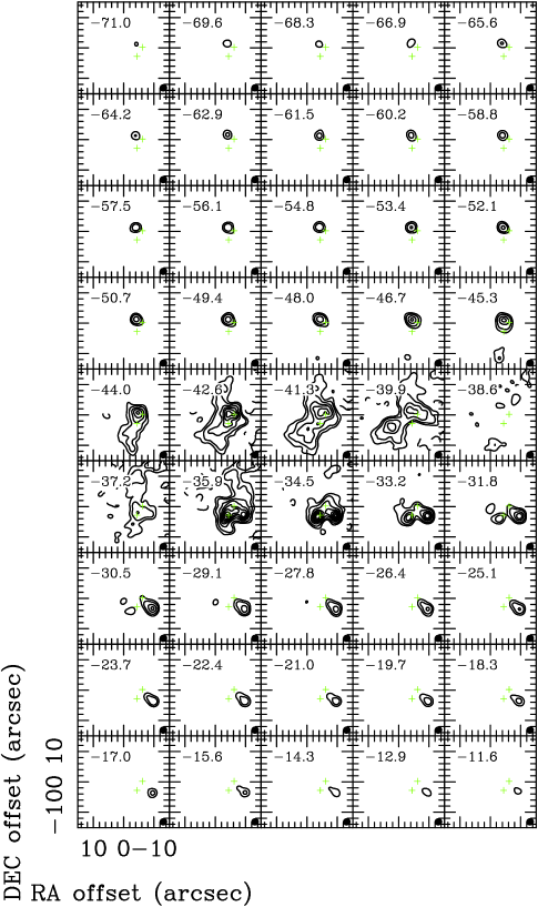
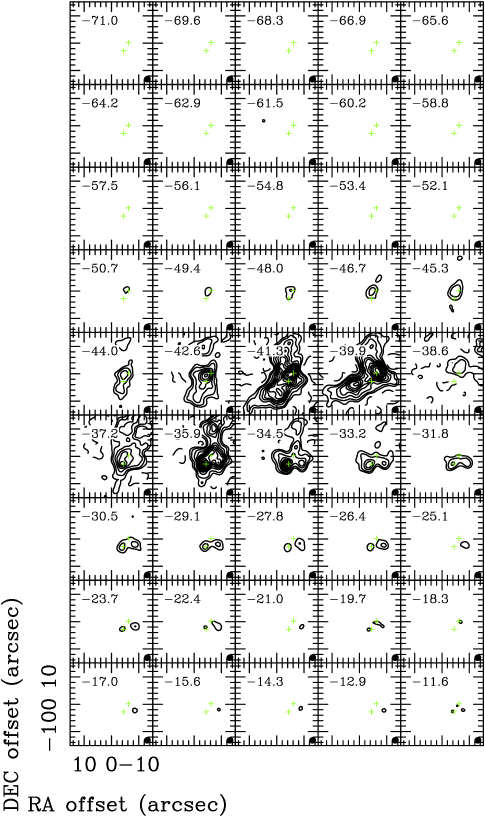
Figure 1.— The channel maps of HCN(3-2) (a: left panel) and HCO⁺(3-2) (b: right panel) with a velocity interval of 1.4 km s^-1. Contours are (-1, 1, 2, 4, 6,…)$\times 5\sigma$, $\sigma$ = 0.045 Jy beam^-1 in both maps with an FWHM beam of 2.5$\arcsec$$\times$2.3$\arcsec$ (–65$\arcdeg$) as marked at right-bottom. The number at left-top in each channel image corresponds to the radial velocity. The green crosses mark the positions of the two proto-stellar objects, SMA-1 and SMA-2.

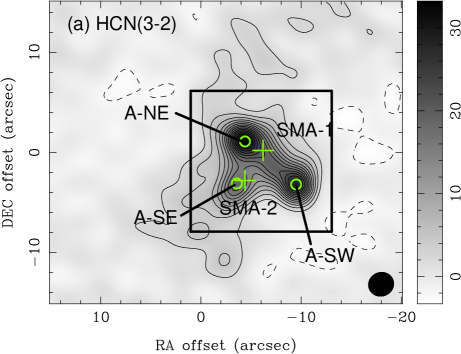
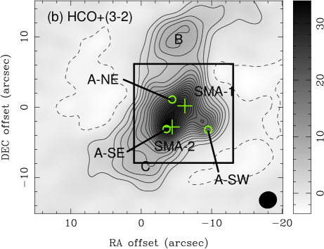
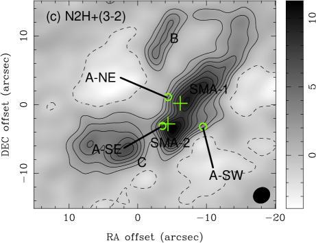
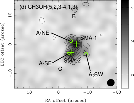
Figure 2.— Integrated intensity maps of (a) HCN(3-2) in the velocity range of (–70.5, –9.8) km s^-1, (b) HCO⁺(3-2) in (–53.0, –21.0) km s^-1, (c) N₂H⁺(3-2) in (–43.5, –34.5) km s^-1 and (d) CH₃OH(5_2,3-4_1,3) in (–44.5, –33.7) km s^-1. Contours are (–1,1,2,3,4…)$\times$3$\sigma$ Jy beam^-1 km s^-1. The rms noises (1 $\sigma$) are $\sim$0.7, $\sim$0.7, $\sim$0.5 and $\sim$0.2 Jy Beam^-1 km s^-1 for the images (a), (b), (c) and (d), respectively. The images (a), (b) and (d) were made from the LSB data observed at $\nu_{\rm LO}=271.7$ GHz with an FWHM beam of $2.5\arcsec\times 2.3\arcsec$ (–65$\arcdeg$). The FWHM beam of the image (c) (USB data) is $2.5\arcsec\times 2.2\arcsec$ (–55$\arcdeg$). Crosses denote the positions of the proto-stellar objects SMA-1 and SMA-2. Open circles mark the three peak positions of the HCN(3-2) line emission (A-NE, A-SW and A-SE). The positions of the weaker emission components B and C observed in HCO⁺(1-0) with the CARMA are also indicated.

Figure 3.— A grid of spectra for the HCN(3-2) line emission. The covered region is marked as the black rectangle in Figure 2a. The pair of numbers in the parenthesis at top-left in each of the spectra gives the offset in units of arcsecond with respect to the reference center.

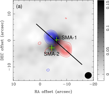
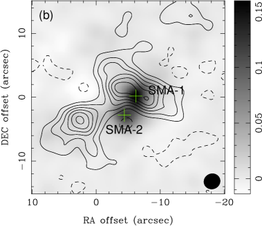
Figure 4.— (a) The high-velocity outflow map in HCN(3-2), integrated from blue wing in the velocity range (–74.1, –45.2) km s^-1 (blue contours) and red wing in (–31.9, –5.8) km s^-1 (red contours). Contours are (-1,1,2,3,4…)$\times$5$\sigma$, 1 $\sigma$ = 0.28 Jy Beam^-1 km s^-1. The position angle of the outflow axis (the thick straight line) is 48$\arcdeg$. (b) The integrated intensity map of the blue-shifted HCN(3-2) emission bump in the velocity range of (–39.9, –39.5) km s^-1, which could somehow trace the distribution of possible infalling gas. Contours are (-1,3,2,3,4…)$\times$3$\sigma$, 1 $\sigma$ = 0.1 Jy Beam^-1 km s^-1. For both the figures the FWHM beam is 2.5$\arcsec$$\times$2.3$\arcsec$, P.A. = –65$\arcdeg$. For both figures the background shows the 1.1-mm continuum distribution, and the wedges are in unit of Jy beam^-1.

Figure 5.— A grid of spectra for the HCO⁺(3-2) line emission. The covered region is marked as the black rectangle in Figure 2b. The pair of numbers in the parenthesis at top-left in each of the spectra gives the offset in units of arcsecond with respect to the reference center.

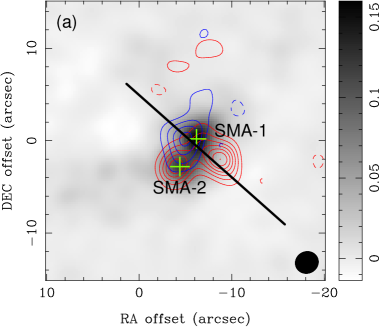
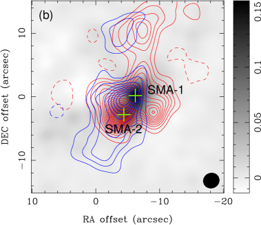
Figure 6.— (a) The high-velocity outflow map in HCO⁺(3-2), integrated from blue wing in the velocity range (–57.9, –45.3) km s^-1 (blue contours) and red wing in (–31.8, –18.8) km s^-1 (red contours). Contours are (-1,1,2,3,4…)$\times$4$\sigma$, 1$\sigma$ = 0.2 Jy Beam^-1 km s^-1. The thick straight line is the same as in Figure 4a. (b) The low-velocity outflow map in HCO⁺(3-2), integrated from blue wing in (–44.9, –41.7) km s^-1 (blue contours) and red wing in (–36.3, –32.3) km s^-1 (red contours). Contours are (-1,1,2,3,4…)$\times$5$\sigma$, 1$\sigma$ = 0.16 Jy Beam^-1 km s^-1. For both the figures the FWHM beam is 2.5$\arcsec$$\times$2.3$\arcsec$, P.A. = –65$\arcdeg$. For both figures the background is the 1.1-mm continuum image, and the wedges are in unit of Jy beam^-1.

Figure 7.— The spectra of HCN(3-2), HCO⁺(3-2), N₂H⁺(3-2) and CH₃OH(5_2,3-4_1,3) (from top to bottom) at SMA-1 (left panels) and SMA-2 (right panels). The vertical dash line in the two figures denotes the peak velocities of the CH₃OH(5_2,3-4_1,3) lines (–39.1 km s^-1), which is used as the systemic velocity through the paper.

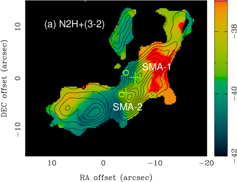
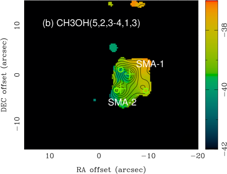
Figure 8.— The centroid velocity maps of (a) N₂H⁺(3-2) and (b) CH₃OH(5_2,3-4_1,3). The contours represent the integrated intensity of the line emission with values of (–1,1,2,3,4…)$\times 3\sigma$ Jy beam^-1 km s^-1 for the given $\sigma=0.5$ and 0.2 Jy beam^-1 km s^-1 with an FWHM beam of $2.5\arcsec\times 2.3\arcsec$ (–65$\arcdeg$) and $2.5\arcsec\times 2.2\arcsec$ (–55$\arcdeg$) in images (a) and (b), respectively. The color wedge scales the radial velocity in the unit of km s^-1.

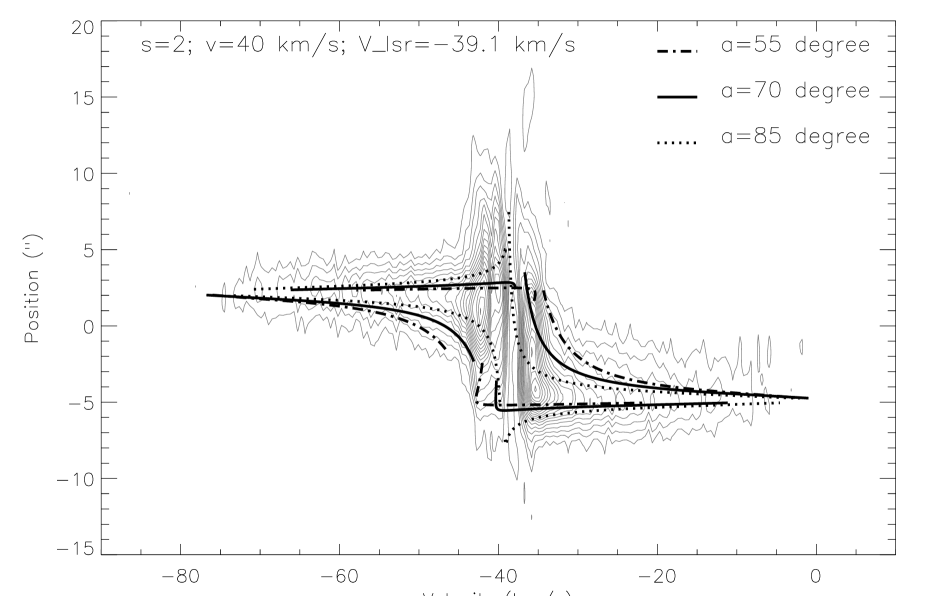
Figure 9.— The position-velocity (P-V) diagram of HCN(3-2) along the outflow axis as indicated with the straight line in Figure 4. The origin in the position axis corresponds to the position of SMA-1 projected on the axis. Contours are 0.2, 0.4, 0.6, 0.8, … Jy beam^-1. The angular and velocity resolutions are 2.7$\arcsec$ and 0.45 km s^-1, respectively. The observed P-V diagram is fitted with the bow-shocked outflow model as discussed in Appendix assuming the systemic velocity in the LSR frame ($V_{\rm sys}=-39.1$ km s^-1), the velocity of the bow-shock ($v=40$ km s^-1), and the spectral index of the power law for the bow-shock surface as function of radius ($s$ = 2). The dashed-dot-dashed, solid, dashed lines stand for the model curves corresponding to the three different values of inclination angle ($\alpha$=55$\arcdeg$, 70$\arcdeg$ and 85$\arcdeg$). The curve with $\alpha$=70$\arcdeg$ appears to represent the best fitting. Note that bow-shock outflow model shows a good fit to the high-velocity gas. The low-velocity gas is probably disturbed by additional processes other than outflow. For example, the emission in the top-left quadrant in the velocities of (–40, –45) km s^-1 and the position offsets of (5$\arcsec$, 6$\arcsec$) are likely from the infalling gas or the gas in the molecular envelope, which is not related to the bow-shock outflow.

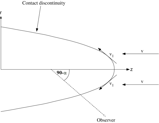
Figure 10.— The sketch illustrates the geometry of the bow-shock outflow model, which is taken from the Figure 6 in Downes & Ray (1999).

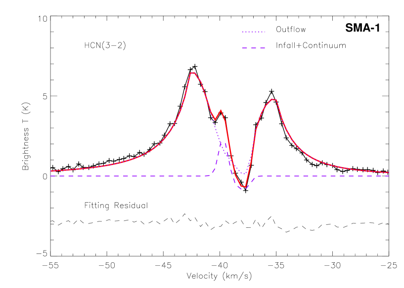
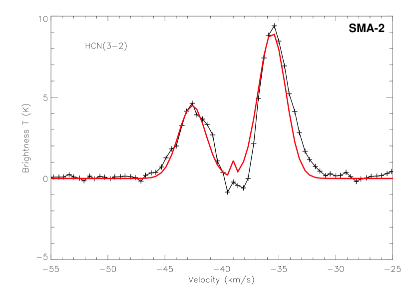
Figure 11.— (a) The observed HCN(3-2) spectral profile towards SMA-1 (solid black curve) is fitted with the four-layer model (red curve) as described by Equation 1, which is discussed in Section 4.2.3 The best fitting gives the optical depths and excitation temperature for the infall gas in front and rear layers ($\tau_{\rm f}=5.0$, $\tau_{\rm r}=0.5$, $J(T_{\rm f})=2$ K, $J(T_{\rm r})=6$ K), and the outflow gas ($\tau_{\rm B}=0.08$, $\tau_{\rm R}=0.06$, $J(T_{\rm out})=76$ K), as well as the dust ($\tau_{\rm c}=0.5$, $J(T_{\rm c})f_{\rm c}=7$ K), respectively. The best fitted velocities and velocity dispersions are ($V_{\rm in}=0.9$ km s^-1, $\sigma_{\rm in}$ = 0.4 km s^-1) and ($V_{\rm out}$ = 3.6 km s^-1, $\sigma_{\rm out}=1.6$ km s^-1) for the infall and the outflow, respectively. The blue dashed and dotted lines represent the best fitted spectral components for the infall and the outflow described in Equation 2, respectively. The line wings are not fitted with the four-layer model; instead, they are simply fitted using a power-law profile with an index of 2. The black dashed line is the residual of subtracting the best fitted model from the data. (b) The observed HCN(3-2) spectral profile towards SMA-2 is fitted to a model with outflow alone ($V_{\rm in}$ = 0 km s^-1) as shown in red curve.

References

- Arce et al. (2006) Arce, H., Shepard, D., Gueth, F., Lee, C.-F., Bachiller, R., Rosen, A., & Beuther, H. 2007, in Protostars and Planets V, ed. B. Reipurth, D. Jewitt, & K. Keil (Tucson, AZ: Univ. Arizona Press), 245
- Attard et al. (2009) Attard, M., Houde, M., Novak, G., Li, H.-B., Vaillancourt, J., Dowell, C. D., Davidson, J. & Shinnaga, H. 2009, ApJ, 702, 1584
- Blitz et al. (1982) Blitz, L., Fich, M. & Stark, A. A. 1982, ApJS, 49, 183
- Bonnell & Bate (2005) Bonnell, I. A. & Bate, M. R. 2005, MNRAS, 362, 915
- Burkert & Bodenheimer (2000) Burkert, A. & Bodenheimer, P. 2000, ApJ, 543, 822
- Caselli et al. (2002) Caselli, P., Benson, P. J., Myers, P. & Tafalla, M. 2002, ApJ, 572, 238
- Di Francesco et al. (2001) Di Francesco, J., Myers, P. C., Wilner, D., Ohashi, N. & Mardones, D. 2001, ApJ, 562, 770
- Downes & Cabrit (2003) Downes, T. P. & Cabrit, S. 2003, RevMexAA, 15, 120
- Downes & Ray (1999) Downes, T. P. & Ray, T. P. 1999, A&A, 345, 977
- Evans et al. (2005) Evans, N. J., II, Lee, J., Rawlings, J. C., & Choi, M. 2005, ApJ, 626, 919
- Goodman et al. (1993) Goodman, A. A., Benson, P. J., Fuller, G. A. & Myers, P. C. 1993, ApJ, 406, 528
- Jorgensen et al. (2004a) Jorgensen, J. K., Hogerheijde, M. R., van Dishoeck, E. F. , Blake, G. A. & Schöier, F. L. 2004, A&A, 413, 993
- Jorgensen et al. (2004b) Jorgensen, J. K., Schöier, F. L. & van Dishoeck, E. F. 2004, A&A, 416, 603
- Lang (1998) Lang, K. R. 1998, Astrophysical Formulae Vol. I (3rd ed.; Berlin: Springer)
- Lay et al. (1995) Lay, O. P., Carlstrom, J. E. & Hills, R. E. 1995, ApJ, 452, L73
- Lee et al. (2000) Lee, C. F., Mundy, L. G., Reipurth, B., Ostriker, E. C. & Stone, J. M. 2000, ApJ, 542, 925
- Lee et al. (2001) Lee, C. F., Stone, J. M., Ostriker, E. C. & Mundy, L. G. 2001, ApJ, 557, 429
- Looney et al. (2000) Looney, L. W., Mundy, L. G. & Welch, W. J. 2000, ApJ, 529, 477
- McKee & Ostriker (2007) McKee, C. F. & Ostriker, E. C. 2007, ARA&A, 45, 565
- Myers et al. (1996) Myers, P. C., Mardones, D., Tafalla, M., Williams, J. P., & Wilner, D. J. 1996, ApJL, 465, L133
- Peretto et al. (2006) Peretto, N., André, P. & Belloche, A. 2006, A&A, 445, 979
- Ruch et al. (2007) Ruch, G. T., Jones, T. J., Woodward, C. E., Polomski, E. F. & Gehrz, R. D. 2007, ApJ, 654, 338
- Sandell et al. (1991) Sandell, G., Aspin, C., Duncan, W. D., Russell, A. P. G. & Robson, E. I. 1991, ApJ, 376, L17
- Sault et al. (1995) Sault, R. J., Teuben, P. J. & Wright, M. C. H. 1995, in Astronomical Society of the Pacific Conference Series, Vol. 77, Astronomical Data Analysis Software and Systems IV, ed. R. A. Shaw, H. E. Payne, & J. J. E. Hayes, 433
- Smith et al. (1997) Smith, M. D., Suttner, G. & Yorke, H. 1997, A&A, 323, 223
- Tohline (2002) Tohline, J. E. 2002, ARA&A, 40, 349
- Ward-Thompson & Buckley (2001) Ward-Thompson, D. & Buckley, H. D. 2001, MNRAS, 327, 955
- Ward-Thompson et al. (1996) Ward-Thompson, D., Buckley, H. D., Greaves, J. S., Holland, W. S. & André, P. 1996, MNRAS, 281, L53
- Wilson et al. (2009) Wilson, T. L., Rohlfs, K. & Hüttemeister, S. 2009, Tools of Radio Astronomy (5th ed.; Berlin: Springer)
- Woods et al. (1975) Woods, R. C., Dixon, T. A., Saykally, R. J. & Szanto, P. G. 1975, PhRvL, 35, 1269
- Wu et al. (2007) Wu, Y., Henkel, C., Xue, R., Guan, X. & Miller, M. 2007, ApJ, 669, L37
- Xu et al. (2006) Xu, Y., Reid, M. J., Zheng, W. W. & Menten, K. M. 2006, Science, 311, 54
- Zhu et al. (2010) Zhu, L., Wright, M., Zhao, J.-H. & Wu., Y. 2010, ApJ, 712, 674