Galaxy And Mass Assembly: Stellar Mass Estimates

Abstract

This paper describes the first catalogue of photometrically-derived stellar mass estimates for intermediate-redshift ($z<0.65$; median $z=0.2$) galaxies in the Galaxy And Mass Assembly (GAMA) spectroscopic redshift survey. These masses, as well as the full set of ancillary stellar population parameters, will be made public as part of GAMA data release 2. Although the GAMA database does include NIR photometry, we show that the quality of our stellar population synthesis fits is significantly poorer when these NIR data are included. Further, for a large fraction of galaxies, the stellar population parameters inferred from the optical–plus–NIR photometry are formally inconsistent with those inferred from the optical data alone. This may indicate problems in our stellar population library, or NIR data issues, or both; hese issues will be addressed for future versions of the catalogue. For now, we have chosen to base our stellar mass estimates on optical photometry only. In light of our decision to ignore the available NIR data, we examine how well stellar mass can be constrained based on optical data alone. We use generic properties of stellar population synthesis models to demonstrate that restframe colour alone is in principle a very good estimator of stellar mass–to–light ratio, $M*/L_{i}$. Further, we use the observed relation between restframe $(g-i)$ and $M_{*}/L_{i}$ for real GAMA galaxies to argue that, modulo uncertainties in the stellar evolution models themselves, $(g-i)$ colour can in practice be used to estimate $M_{*}/L_{i}$ to an accuracy of $\lesssim 0.1$ dex (1$\sigma$). This ‘empirically calibrated’ $(g-i)$–$M_{*}/L_{i}$ relation offers a simple and transparent means for estimating galaxies’ stellar masses based on minimal data, and so provides a solid basis for other surveys to compare their results to $z\lesssim 0.4$ measurements from GAMA.

1 Introduction

One of the major difficulties in observationally constraining the formation and evolutionary histories of galaxies is that there is no good observational tracer of formation time or age. In the simplest possible terms, galaxies grow through a combination of continuous and/or stochastic star formation and episodic mergers. Throughout this process—and in contrast to other global properties like luminosity, star formation rate, restframe colour, or luminosity-weighted mean stellar age—a galaxy’s evolution in stellar mass is nearly monotonic and relatively slow. Stellar mass thus provides a good, practical basis for evolutionary studies.

Further, it is now clear that stellar mass plays a central role in determining—or at least describing—a galaxy’s evolutionary state. Virtually all of the global properties commonly used to describe galaxies—e.g., luminosity, restframe colour, size, structure, star formation rate, mean stellar age, metallicity, local density, and velocity dispersion or rotation velocity—are strongly and tightly correlated (see, e.g., Minkowski, 1962; Faber & Jackson, 1976; Tully & Fisher, 1977; Sandage & Visvanathan, 1978; Dressler, 1980; Djorgovsky & Davis, 1987; Dressler et al., 1987; Strateva et al., 2001). One of most influential insights to come from the ambitious wide- and deep-field galaxy censuses of the 2000s has been the idea that most, if not all, of these correlations can be best understood as being primarily a sequence in stellar mass (e.g. Shen et al., 2003; Kauffmann et al., 2003b, 2004; Tremonti et al., 2004; Blanton et al., 2005; Baldry et al., 2006; Gallazzi et al., 2006). Given a galaxy’s stellar mass, it is thus possible to predict most other global properties with considerable accuracy. Presumably, key information about the physical processes that govern the process of galaxy formation and evolution are encoded in the forms of, and scatter around, these stellar mass scaling relations.

1.1 Galaxy And Mass Assembly (GAMA)

This paper presents the first catalogue of stellar mass estimates for galaxies in the Galaxy And Mass Assembly (GAMA) survey (Driver et al., 2009, 2011). At its core, GAMA is an optical spectroscopic redshift survey, specifically designed to have near total spectroscopic completeness over cosmologically representative volume. In terms of survey area and target surface density, GAMA is intermediate and complementary to wide-field, low-redshift galaxy censuses like SDSS (York et al., 2000; Strauss et al., 2002; Abazajian et al., 2009), 2dFGRS (Colless et al., 2001, 2003; Cole et al., 2005), 6dFGS (Jones et al., 2004, 2009), or the MGC (Liske et al., 2003; Driver et al., 2005) and deep-field surveys of the high redshift universe like VVDS (Le Fèvre et al., 2005), DEEP-2 (Davis et al., 2003), COMBO-17 (Wolf et al., 2003, 2004), COSMOS and zCOSMOS (Scoville et al., 2007; Lilly et al., 2007). The intermediate redshift regime ($z\lesssim 0.3$) that GAMA probes is thus largely unexplored territory: GAMA provides a unique resource for studies of the evolving properties of the general galaxy population.

In a broader sense, GAMA aims to unite data from a number of large survey projects spanning nearly the full range of the electromagnetic spectrum, and using many of the world’s best telescopes. At present, the photometric backbone of the dataset is optical imaging from SDSS and near infrared (NIR) imaging taken as part of the Large Area Survey (LAS) component of the UKIRT Infrared Deep Sky Survey (UKIDSS; Dye et al., 2006; Lawrence et al., 2007). GALEX UV imaging from the Medium Imaging Survey (MIS; Martin et al., 2005; Morrissey et al., 2007) is available for the full GAMA survey region. At longer wavelengths, mid-infrared imaging is available from the WISE all-sky survey (Wright et al., 2010), far infrared imaging is available from the Herschel-ATLAS project (Eales et al., 2010), and metre-wavelength radio imaging is being obtained using the Giant Metre-wave Radio Telescope (GMRT; PI: M. Jarvis). In the near future, the SDSS and UKIDSS imaging will be superseded by significantly deeper, sub-arcsecond resolution imaging from the VST-KIDS project (PI: K. Kuijken) and from the VISTA-VIKING survey (PI: W. Sutherland). Looking slightly further ahead, a subset of the GAMA fields will also be targeted by the ASKAP-DINGO project (PI: M. Meyer), adding 21 cm data to the mix. By combining these many different datasets into a single and truly panchromatic database, GAMA aims to construct ‘the ultimate galaxy catalogue’, offering the first laboratory for simultaneously studying the AGN, stellar, dust, and gas components of large and representative samples of galaxies at low-to-intermediate redshifts.

The stellar masses estimates, as well as estimates for ancillary stellar popualtion parameters like age, metallicity, and restframe colour, form a crucial part of the GAMA value-added dataset. These values are already in use within the GAMA team for a number of science applications.. In keeping with GAMA’s commitment to providing these data as a useful and freely available resource, the stellar mass estimates described in this paper are being made publicly available as part of the GAMA data release 2, scheduled for mid-2011. Particularly in concert with other GAMA value-added catalogues, and with catalogues from other wide- and deep-field galaxy surveys, the GAMA stellar mass estimates are intended to provide a valuable public resource for studies of galaxy formation and evolution. A primary goal of this paper is therefore to provide a standard reference for users of these catalogues.

1.2 Stellar mass estimation

Stellar mass estimates are generally derived through stellar population synthesis (SPS) modelling (Tinsley & Gunn, 1976; Tinsley, 1978; Bruzual, 1993). This technique relies on stellar evolution models (e.g., Leitherer et al., 1999; Le Borgne & Rocca-Volmerange, 2002; BC03, ; M05, ; Percival et al., 2009). Assuming a stellar initial mass function (IMF), these models describe the spectral evolution of a single-aged or simple stellar population (SSP) as a function of its age and metallicity. The idea behind SPS modelling is to combine the individual SSP models according to some fiducial star formation history (SFH), and so to construct composite stellar populations (CSPs) that match the observed properties of real galaxies. The stellar population (SP) parameters—including stellar mass, star formation rate, luminosity weighted mean stellar age and metallicity, and dust obscuration—implied by such a fit can then be ascribed to the galaxy in question (see, e.g. Brinchmann & Ellis, 2000; Cole et al., 2001; Bell et al., 2003; Kauffmann et al., 2003a; Gallazzi et al., 2005).

SPS fitting is most commonly done using broadband spectral energy distributions (SEDs) or spectral indices (see the comprehensive review by Walcher et al., 2011). This presents two interrelated challenges. First is the question of the accuracy and reliability of the spectral models that make up the stellar population library (SPL) used as the basis of the fitting, including both the stellar evolution models that underpin the synthetic spectra, and the SFHs used to construct the SPL. Second, there is the question of what SED or spectral features provide the strongest and/or most robust constraints on a galaxy’s SP, taking into account the uncertainties and assumptions intrinsic to the models.

In principle, the accuracy of SPS-derived parameter estimates is limited by generic degeneracies between different SP models with the same or similar observable properties—for example, the well known dust–age–metallicity degeneracy (see, e.g., Worthey, 1994). Further, the SPS fitting problem is typically badly under-constrained, inasmuch as it is extremely difficult to place meaningful constraints on a given galaxy’s particular SFH. This issue has been recently explored by Gallazzi & Bell (2009), who tested their ability to recover the known SP parameters of mock galaxies, in order to determine the limiting accuracy of stellar mass estimates. In the highly idealised case that the SPL contains a perfect description of each and every galaxy, and that the photometry is perfectly calibrated, and that the dust extinction is known exactly, Gallazzi & Bell (2009) argue that SP model degeneracies mean that both spectroscopic and photometric stellar mass estimates are generically limited to an accuracy of $\lesssim 0.2$ dex for galaxies with a strong burst component, and $\sim 0.10$ dex otherwise.

In practice, the dominant uncertainties in SPS-derived parameter estimates are likely to come from uncertainties inherent to the SP models themselves. Despite the considerable progress that has been made, there remain a number of important ‘known unknowns’. The form and universality (or otherwise) of the stellar IMF is a major source of uncertainty (Wilkins et al., 2008; van Dokkum, 2008; Gunawardhana et al., 2011). From the stellar evolution side, the treatment of NIR-luminous thermally pulsating asymptotic giant branch stars (TP-AGBs; M05, ; Maraston, 2006; Kriek et al., 2010) is the subject of some controversy. As a third example, there is the question of how to appropriately model the effects of dust in the interstellar medium (ISM), including both the form of the dust obscuration/extinction law, and the precise geometry of the dust with respect to the stars (Driver et al., 2007; Wuyts et al., 2009; Wijesinghe et al., 2011). Many of these uncertainties and their propagation through to stellar mass estimates are throughly explored and quantified in the excellent work of Conroy, Gunn & White (2009); Conroy & Gunn (2010), who argue that (when fitting to full UV–to–NIR SEDs) the net uncertainty in any individual $z\sim 0$ stellar mass determination is on the order of $\lesssim 0.3$ dex.

Differential systematic errors across galaxy populations—that is, biases in the stellar masses of different galaxies as a function of mass, age, SFH, etc.—are at least as great a concern as the net uncertainty on any individual galaxy. The vast majority of stellar mass-based science focusses on differences in the (average) properties of galaxies as a function of inferred mass. In such comparative studies, differential biases have the potential to induce a spurious signal, or, conversely, to mask true signal. In this context, Taylor et al. (2010b) have used the consistency between stellar and dynamical mass estimates for SDSS galaxies to argue that any such differential biases in $M_{*}/L_{i}$ (cf. $M_{*}$) as a function of stellar population are limited to $\lesssim 0.12$ dex (40 %); i.e., small.

In a similar way, systematic differential biases in the masses and SP parameters of galaxies at different redshifts are a major concern for evolutionary studies, inasmuch as any such redshift-dependent biases will induce a false evolutionary signal. Indeed, for the specific example of measurement of the evolving comoving number density of massive galaxies at $z\lesssim 2$, such differential errors are the single largest source of uncertainty, random or systematic (Taylor et al., 2009). More generally, such differential biases will be generically important whenever the low redshift point makes a significant contribution to the evolutionary signal; that is, whenever the amount of evolution is comparable to the random errors on the high redshift points. In this context, by probing the intermediate redshift regime and providing a link between $z\approx 0$ surveys like SDSS and 2dFGRS and $z\gg 0$ deep surveys like VVDS and DEEP-2, GAMA makes it possible to identify and correct for any such differential effects. GAMA thus has the potential to significantly reduce or even eliminate a major source of uncertainty for a wide variety of lookback survey results.

1.3 This work

Before we begin, a few words on the ethos behind our SPS modelling procedure: we have deliberately set out to do things as simply and as conventionally as is possible and appropriate. There are two main reasons for this decision. First, this is only the first generation of stellar mass estimates for GAMA. We intend to use the results presented here to inform and guide future improvements and refinements to our SPS fitting algorithm. Second, in the context of studying galaxy evolution, GAMA’s unique contribution is to probe the intermediate redshift regime; GAMA becomes most powerful when combined with very wide low redshift galaxy censuses on the one hand, and with very deep lookback surveys on the other. To maximise GAMA’s utility, it is therefore highly desirable to provide masses that are directly comparable to estimates used by other survey teams. This includes using techniques that are practicable for high redshift studies.

With all of the above as background, the programme for this paper is as follows. After describing the subset of the GAMA database that we will make use of in §2, we lay out our SPS modelling procedure in §3. In particular, in §3.4, we show the importance of taking a Bayesian approach to SP parameter estimation.

In §4, we look at how our results change with the inclusion of NIR data. Specifically, in §4.1, we show that our SPL models do not yield a good description of the GAMA optical–to–NIR SED shapes. Further, in §4.2, we show that for a large fraction of galaxies, the SP parameter values derived from the full optical–plus–NIR SEDs are formally inconsistent with those derived from just the optical data. Both of these statements are true irrespective of the choice of SSP models used to construct the SPL (§4.3).

In order to interpret the results presented in §4, we have conducted a set of numerical experiments designed to test our ability to fit synthetic galaxies photometry, and to recover the ‘known’ SP parameters of mock galaxies. Based on these tests, which we describe in Appendix A, we have no reason to expect the kinds of differences found in §4—we therefore conclude that, at least for the time being, it is better for us to ignore the available NIR data §4.5.

In light of our decision not to use the available NIR data, in §5, we investigate how well optical data can be used to constrain a galaxy’s $M_{*}/L$. Using the SPL models, we show in §5.2 that, in principle, $(g-i)$ colour can be used to estimate $M_{*}/L_{i}$ to within a factor of $\lesssim 2$. In §5.3, we use the empirical relation between ($ugriz$-derived) $M_{*}/L_{i}$ and $(g-i)$ colour to show that, in practice, $(g-i)$ can be used to infer $M_{*}/L_{i}$ to an accuracy of $\approx 0.1$ dex. The derived colour–$M/L$ relation presented in this section is provided to enable meaningful comparison between stellar mass-centric measurements from GAMA and other surveys.

Finally, in §6, we discuss how we might improve on the current SP parameter estimates for future catalogues. In particular, in §6.2, we examine potential causes and solutions for our current problems in incorporating the NIR data. In this section, we suggest that we have reached the practical limit for SP parameter estimation based on grid-search-like algorithms using a static SPL. In order to improve on the current estimates, future efforts will require a fundamentally different conceptual approach. However, as we argue in §6.1, this will not necessarily lead to significant improvements in the robustness or reliability of our stellar mass estimates.

Separately, we compare the SDSS and GAMA photometry and stellar mass estimates in Appendix B. Despite there being large and systematic differences between the SDSS model and GAMA auto SEDs, we find that the GAMA- and SDSS-derived $M_{*}/L$s are in excellent agreement. On the other hand, we also show that, as a measure of total flux, the SDSS model photometry suffers from structure-dependent biases; the differential effect is at the level of a factor of 2. These large and systematic biases in total flux translate directly to biases in the inferred total mass. For SDSS, this may in fact be the single largest source of uncertainties in their stellar mass estimates. In principle, this will have a significant impact on stellar mass-centric measurements based on SDSS data.

Throughout this work, we adopt the concordance cosmology: $(\Omega_{\Lambda},~{}\Omega_{m},~{}h)=(0.7,~{}0.3,~{}0.7)$. Different choices for the value of $h$ can be accommodated by scaling any and all absolute magnitudes or total stellar masses by $+5\log h/0.7$ or $-2\log h/0.7$, respectively (i.e., a higher value of the Hubble parameter implies a lower luminosity or total mass). All other SP parameters, including restframe colours, ages, dust extinctions, and mass-to-light ratios can be taken to be cosmology-independent, inasmuch as they pertain to the stellar populations at the time of observation. We assume a Chabrier (2003) IMF. Our stellar mass estimates are based on the BC03 SP models and the dust obscuration law of Calzetti et al. (2000). We briefly consider the effect of using the M05 or CB07 SP models on the inferred SP parameter estimates in §4.3. In discussions of stellar mass-to-light ratios, we use $M_{*}/L_{X}$ to denote the ratio between stellar mass and luminosity in the restframe $X$-band; where the discussion is generic to all (optical and NIR) bands, we will drop the subscript for convenience. In all cases, the $L_{X}$ in $M_{*}/L_{X}$ should be understood as referring to the absolute luminosity of the galaxy, i.e., without correction for internal dust extinction. We thus consider effective, and not intrinsic stellar mass-to-light ratios. Unless explicitly stated otherwise, quantitative values of $M_{*}/L_{X}$s are given using units of $L_{X}$ equivalent to an AB magnitude of 0 (rather than, say, $L_{\odot,X}$). All quoted magnitudes use the AB system.

2 Data

2.1 Spectroscopic redshifts

The lynchpin of the GAMA dataset is a galaxy redshift survey targeting three $4^{\circ}\times 12^{\circ}$ equatorial fields centred on $9^{\mathrm{h}}00^{\mathrm{m}}+1^{\mathrm{d}}$, $12^{\mathrm{h}}00^{\mathrm{m}}+0^{\mathrm{d}}$, and $14^{\mathrm{h}}30^{\mathrm{m}}+0^{\mathrm{d}}$ (dubbed G09, G12, and G15, respectively), for an effective survey area of 144 $\square^{\circ}$. Spectra were taken using the AAOmega spectrograph (Saunders et al., 2004; Sharp et al., 2006), which is fed by the 2dF fibre positioning system on the 4m Anglo-Australian Telescope (AAT). The algorithm for allocating 2dF fibres to survey targets, described by Robotham et al. (2010) and implemented for the second and third years of observing, was specifically designed to optimise the spatial completeness of the final catalogue. Observations were made using AAOmega’s 580V and 385R gratings, yielding continuous spectra over the range 3720–8850 Å with an effective resolving power of $R\approx 1300$. Observations for the first phase of the GAMA project, GAMA I, have recently been completed in a 68 night campaign spanning 2008–2010. GAMA has just been awarded AAT long term survey status with a view to trebling its survey volume; observations for GAMA II are underway, and will be completed in 2012.

Target selection for GAMA I has been done on the basis of optical imaging from SDSS (DR6; Adelman-McCarthy et al., 2009) and NIR imaging from UKIRT, taken as part of the UKIDSS LAS (Dye et al., 2006; Lawrence et al., 2007). The target selection is described in full by Baldry et al. (2010). In brief, the GAMA spectroscopic sample is primarily selected on $r$-band magnitude, using the (Galactic/foreground extinction-corrected) petro magnitudes given in the basic SDSS catalogue. The main sample is magnitude-limited to $r_{\mathtt{petro}}<19.4$ in the G09/G15 fields, and $r_{\mathtt{petro}}<19.8$ in G12. (The definitions of the SDSS petro and model magnitudes can be found in §B.1.) In order to increase the stellar mass completeness of the sample, there are two additional selections: $z_{\mathtt{model}}<18.2$ or $K_{\mathtt{auto}}<17.6$ (AB). For these two additional selections, in order to ensure both photometric reliability and a reasonable redshift success rate, it is also required that the $r_{\mathtt{model}}<20.5$. The effect of these additional selections is to increase the target density marginally by $\sim 7$ % (1 %) in the G09/G15 (G12) fields. Star–galaxy separation is done based on the observed shape in a similar manner as for the SDSS (see Baldry et al., 2010; Strauss et al., 2002, for details), with an additional $(J-K)$–$(g-i)$ colour selection designed to exclude those double/blended stars that still fall on the stellar locus in colour–colour space.

To these limits, the survey spectroscopic completeness is high ($\gtrsim 98$ %; see Driver et al., 2011; Liske et al., in prep.). The issue of photometric incompleteness in the target selection catalogues has been investigated by Loveday et al. (in prep.) using SDSS Stripe 82: the SDSS imaging completeness is $>99$ (90) % for $\mu<22.5$ (23) mag/$\square^{\prime\prime}$.

The process for the reduction and analysis of the AAOmega spectra is described in Driver et al. (2011). All redshifts have been measured by GAMA team members at the telescope, using the interactive redshifting software RUNZ (developed by Will Sutherland and now maintained by Scott Croom). For each reduced and sky-subtracted spectrum, RUNZ presents the user with a first redshift estimate. Users are then free to change the redshift in the case that the RUNZ-derived redshift is deemed incorrect, and are always required to give a subjective figure of merit for the final redshift determination.

To ensure the uniformity and reliability of both the redshifts and the quality flags, a large subset (approximately 1/3, including all those with redshifts deemed ‘maybe’ or ‘probably’ correct) of the GAMA spectra have been independently ‘re-redshifted’ by multiple team members. The results of the blind re-redshifting are used to derive a probability for each redshift determination, $p_{z}$, which also accounts for the reliability of the individual who actually determined the redshift (Liske et al., in prep.). The final values of the redshifts and quality flags, nQ, given in the GAMA catalogues are then based on these ‘normalised’ probabilities. (Note that this work makes use of ‘year 3’ redshifts, which have yet not undergone the re-redshifting process.) Driver et al. (2011) suggests that the redshift ‘blunder’ rate for galaxies with $\mathtt{nQ}=3$ (corresponding to $0.90<p_{z}<0.95$) is in the range 5–15 %, and that for $\mathtt{nQ}=4$ (corresponding to $p_{z}>0.95$) is 3–5 %. A more complete analysis of the GAMA redshift reliability will be provided by Liske et al. (in prep.).

The redshifts derived from the spectra are, naturally, heliocentric. For the purposes of calculating luminosity distances (see §3.2), we have computed flow-corrected redshifts using the model of Tonry et al. (2000). The details of this conversion will be given by Baldry et al. (in prep.).

The GAMA I main galaxy sample ($\mathtt{SURVEY\_CLASS}\geq 4$ in the GAMA catalogues) comprises 119852 spectroscopic targets, of which 94.5 % (113267/119852) now have reliable ($\mathtt{nQ}\geq 3$) spectroscopic redshifts. Of the reliable redshifts, 83 % (94448/113267) are measurements obtained by GAMA. The remainder are taken from previous redshift surveys, principally SDSS (DR7 Abazajian et al., 2009, 13137 redshifts), 2dFGRS (Colless et al., 2003, 3622 redshifts), and MGCz (Driver et al., 2005, 1647 redshifts). As a function of SDSS fiber magnitude (taken as a proxy for the flux seen by the $2^{\prime\prime}$ 2dF spectroscopic fibres), the GAMA redshift success rate ($\mathtt{nQ}\geq 3$) is essentially 100 % for $r_{\mathtt{fiber}}<19.5$, dropping to 98 % for $r_{\mathtt{fiber}}=20$, and then down to $\sim 50$ % for $r_{\mathtt{fiber}}=22$ (Loveday et al., in prep.). For the $r$-selected survey sample ($\mathtt{SURVEY\_CLASS}\geq 6$), the net redshift success rate is 95.4 % (109222/114250).

Stellar mass estimates have been derived for all objects with a spectroscopic redshift $0<z\leq 0.65$. For the purposes of this work, we will restrict ourselves to considering only those galaxies with $z>0.002$ (to exclude stars), and those galaxies with $\mathtt{nQ}\geq 3$ (to exclude potentially suspect redshift determinations). We quantify the sample completeness in terms of stellar mass, restframe colour, and redshift in §3.5.

2.2 Broadband Spectral Energy Distributions (SEDs)

This work is based on version 6 of the GAMA master catalogue (internal designation catgama_v6), which contains $ugrizYJHK$ photometry for galaxies in the GAMA regions. The photometry is based on SDSS (DR7) optical imaging, and UKIDSS LAS (DR4) NIR imaging. The SDSS data have been taken from the Data Archive Server (DAS); the UKIDSS data have been taken from the WFCAM Science Archive (WSA; Hambly et al., 2008).

In each case, the imaging data are publicly available in a fully reduced and calibrated form. The SDSS data reduction has been extensively described (see, e.g. Strauss et al., 2002; Abazajian et al., 2009). The LAS data have been reduced using the WFCAM-specific pipeline developed and maintained by the Cambridge Astronomical Survey Unit (CASU).

The GAMA photometric catalogue is constructed from an independent reanalysis of these imaging data. The data and the GAMA reanalysis of them are described fully by Hill et al. (2010) and Kelvin et al. (in prep.). We summarise the most salient aspects of the GAMA photometric pipeline below. As described in Hill et al. (2010), the data in each band are normalised and combined into three astrometrically matched Gigapixel-scale mosaics (one for each of the G09, G12, and G15 fields), each with a scale of $0\aas@@fstack{\prime\prime}4$ pix^-1. In the process of the mosaicking, individual frames are degraded to a common seeing of 2^′′ FWHM.

Photometry is done on these PSF-matched images using SExtractor (Bertin & Arnouts, 1996) in dual image mode, using the $r$-band image as the detection image. For this work, we construct multicolour SEDs using SExtractor’s auto photometry. This is a flexible, elliptical aperture whose size is determined from the observed light distribution within a quasi-isophotal region (see Bertin & Arnouts, 1996; Kron et al., 1980, for further explanation) of the $r$-band detection image. This provides seeing- and aperture-matched photometry in all bands.

In addition to the matched-aperture photometry, the GAMA catalogue also contains $r$-band Sérsic-fit structural parameters, including total magnitudes, effective radii, and Sérsic indices (Kelvin et al., in prep.). These values have been derived using GALFIT3 (Peng et al., 2002) applied to (undegraded) mosaics constructed in the same manner as those described above. These fits incorporate a model of the PSF for each image, and so should be understood to be seeing corrected. In estimating total magnitudes, the Sérsic models have been truncated at 10 $R_{\mathrm{e}}$; this typically corresponds to a surface brightness of $\mu_{r}\sim 30$ mag / $\square^{\prime\prime}$. Hill et al. (2010) present a series of detailed comparisons between the different GAMA and SDSS/UKIDDS photometric measures. Additional comparisons between the GAMA and SDSS optical photometry are presented in Appendix B. In this work, we use these $r$-band sersic magnitudes to estimate galaxies’ total luminosities, since these measurements (attempt to) account for flux missed by the finite auto apertures.

For each galaxy, we construct multicolour SEDs using the SExtractor auto aperture photometry. Formally, when fitting to these SEDs, we are deriving SP parameters integrated or averaged over the projected auto aperture. In order to get an estimate of a galaxy’s total stellar mass, it is therefore necessary to scale the inferred mass up, so as to account for flux/mass lying beyond the (finite) auto aperture. We do this by simply scaling each of the auto fluxes by the amount required to match the $r$-band auto aperture flux to the sersic measure of total flux; i.e., using the scalar aperture correction factor $f_{\mathrm{ap}}=10^{-0.4(r_{\mathtt{auto}}-r_{\mathtt{sersic}})}$.

Note that we elect not to use the NIR data to derive stellar mass estimates for the current generation of the GAMA stellar mass catalogue. Our reasons for this decision are the subject of §4.

3 Stellar Population Synthesis (SPS) modelling and stellar mass estimation

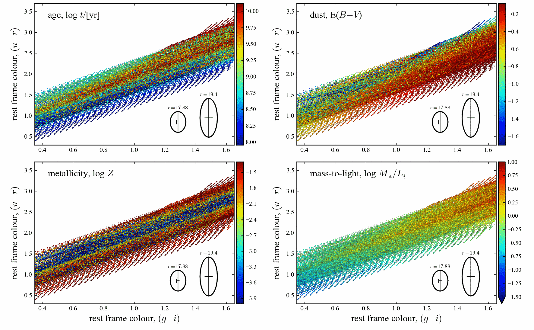
Figure 1: Illustrating the basic idea behind stellar population synthesis modelling.— In each panel of this Figure, we plot the restframe $(u-r)$ and $(g-i)$ colours of the models in our library, colour-coded by an important basic property: CSP age, $t$, dust obscuration, $\mathrm{E}_{B\text{-}V}$, stellar metallicity, $Z$, and mass-to-light ratio, $M_{*}/L_{i}$. In the simplest terms possible, given a galaxy’s restframe $(ugri)$ photometry, the process of stellar population parameter estimation can be thought of as just ‘reading off’ the value of each parameter. For comparison, the the median 1$\sigma$ uncertainty in the observer’s frame $ugri$ colours for GAMA galaxies at the SDSS and GAMA spectroscopic selection limits ($m_{r}=17.88$ and $19.4$, respectively) are shown in each panel. Note that, as is standard practice, we impose an error floor of 0.05 mag in the photometry in each band; the ellipses show the effective uncertainties with the inclusion of this error floor. With the exception of the $u$ band, the catalogued error is almost always less than 0.05 mag; these errors are shown as the error bars within each ellipse. We are limited not by random noise, but by the systematic errors in the relative or cross-calibration of the photometry in the different bands. In each panel, areas where one colour dominates shows where a given parameter can be well constrained using $ugri$ photometry. Conversely, where models with similar $ugri$ colours have a wide range of parameter values, this parameter cannot be well constrained. Thus it can be seen that even though $t$, $\mathrm{E}_{B\text{-}V}$, and particularly $Z$ are generally not well constrained from an optical SED, $M_{*}/L$ can still be relatively robustly estimated.

The essential idea behind SPS modelling is to determine the characteristics of the SPs that best reproduce the observed properties (in our case, the broadband spectral energy distribution; SED) of the galaxy in question. As an illustrative introduction to the problem, Figure 1 shows the distribution of our SPS model templates in restframe $(u-r)$–$(g-i)$ colour–colour space. In each panel of this Figure, we colour-code each model according to a different SP parameter.

Imagine for a moment that instead of using the observed $ugriz$ SEDs, we were to first transform those SEDs into restframe $ugri$ photometry, and then use this as the basis of the SPS fitting. In the simplest possible terms, the fitting procedure could then be thought of as ‘reading off’ the parameters of the model(s) found in the region of the $ugri$ colour–colour space inhabited by the galaxy.

In this Figure, regions that are dominated by a single colour show where a parameter can be tightly constrained on the basis of a (restframe) $ugri$ SED. Conversely, regions where the different colours are well mixed show where models with a wide range of parameter values provide equally good descriptions of a given $ugri$ SED shape; that is, where there are strong degeneracies between model parameters.

In general terms, then, Figure 1 demonstrates that it is difficult to derive strong constraints on $t$ or $Z$; this is the well known age–metallicity degeneracy. Even where such strong degeneracies exist, however, note that the value of $M_{*}/L$ is considerably better constrained than any of the parameters that are used to define each model.

3.1 Synthetic stellar population models

The fiducial GAMA stellar mass estimates are based on the BC03 synthetic SP model library, which consists of spectra for single-aged or simple stellar populations (SSPs), parameterised by their age, $t$, and metallicity, $Z$; i.e., $f_{\mathrm{SSP}}(\lambda;~{}t,~{}Z)$. Given these SSP spectra and an assumed star formation history (SFH), $\psi_{*}(t)$, spectra for composite stellar populations (CSPs) can be constructed, as a linear combination of different simple SSP spectra; i.e.:

$$f_{\mathrm{CSP}}(\lambda;~{}Z,~{}t,~{} \mathrm{E}_{B\text{-}V})=$$

$$k(\lambda;~{} \mathrm{E}_{B\text{-}V})\int\limits_{t^{\prime}=0}^{t}\mathrm{d}t^{\prime}~{}\psi_{*}(t^{\prime})\times f_{\mathrm{SSP}}(\lambda;~{}Z,~{}t^{\prime})~{}.$$ (1)

Here, $k(\lambda;~{}\mathrm{E}_{B\text{-}V})$ is a single-screen dust attenuation law, where the degree of attenuation is characterised by the selective extinction between the $B$ and $V$ bands, $\mathrm{E}_{B\text{-}V}$. Note that this formalism works for any quantity that is additive; e.g. flux in a given band, stellar mass (including sub-luminous stars, and accounting for mass loss as a function of SSP age), the mass contained in stellar remnants (including white dwarfs, black holes), etc.

When using this Equation to construct the CSP models that comprise our SPL, we make three simplifying assumptions. We consider only smooth, exponentially-declining star formation histories, which parameterised by the $e$-folding timescale, $\tau$; i.e., $\psi_{*}(t)\propto e^{-t/\tau}$. We make the common assumption that each CSP has a single, uniform stellar metallicity, $Z$. We also make the (equally common) assumption that a single dust obscuration correction can be used for the entire CSP.

For our fiducial mass estimates, we use a Calzetti et al. (2000) dust attenuation ‘law’. In this context, we highlight the work of Wijesinghe et al. (2011), who look at the consistency of different dust obscuration laws in the optical and ultraviolet. They conclude that the Fischera & Dopita (2005) dust curve is best able to describe the optical–to–ultraviolet SED shapes of GAMA galaxies. In the optical, the shapes of the Fischera & Dopita (2005) and Calzetti et al. (2000) curves are quite similar. Using the Fischera & Dopita (2005) curve does not significantly alter our results.

The models in our SPL are thus characterised by four key parameters: age, $t$; $e$-folding time, $\tau$; metallicity, $Z$; and dust obscuration, $\mathrm{E}_{B\text{-}V}$. In an attempt to cover the full range of possible stellar populations found in real galaxies, we construct a library of CSP model spectra spanning a semi-uniform grid in each parameter. The age grid spans the range $\log t/\left[\mathrm{yr}\right]=8$–8.9 in steps of 0.1 dex, then from $\log t/\left[\mathrm{yr}\right]=9$–10.10 in steps of 0.05 dex, and then with a final value of 10.13 ($\approx 13.4$ Gyr). The grid of $e$-folding times spans the range $\log\tau/\left[\mathrm{yr}\right]=7.5$–8.9 in steps of 0.2 dex, and then from $\log\tau/\left[\mathrm{yr}\right]=9$–10 in steps of 0.1 dex. The dust grid covers the range $\mathrm{E}_{B\text{-}V}=0.0$–$0.8$ in steps of 0.02 mag. We use the native metallicity grid for the BC03 models: $Z=$ (0.0001, 0.0004, 0.004, 0.008, 0.02, 0.05). The fiducial model grid thus includes $34\times 19\times 43\times 6=166668$ models for each of 66 redshifts between $z=0.00$ and $0.65$, for a total of just over 11 million individual sets of 9 band synthetic photometry.

3.2 SED fitting

Synthetic broadband photometry is derived using the CSP spectra and a model for the total instrumental response for each of the $ugriz$- and $YJHK$-bands. The optical and NIR filter response functions are taken from Doi et al. (2010) and from Hewett et al. (2006), respectively. These curves account for atmospheric transmission (assuming an airmass of 1.3), filter transmission, mirror reflectance, and detector efficiency, all as a function of wavelength. For a given a template spectrum $f_{\mathrm{CSP}}$, placed at redshift $z$, the template flux in the (observers’ frame) $X$-band, $T_{X}$, is then given by:

$$T_{X}(\mathrm{CSP};z)=(1+z)~{}\frac{\int\mathrm{d}{\lambda}~{}r_{X}(\lambda)~{}\lambda~{}f_{\mathrm{CSP}}(\frac{\lambda}{1+z})}{\int\mathrm{d}{\lambda}~{}r_{X}(\lambda)~{}\lambda}~{}.$$ (2)

Here, $r_{X}$ is filter response function, and the prefactor of $(1+z)$ accounts for the redshift-stretching of the bandpass interval. Also note that the factor of $\lambda$ in both integrals is required to account for the fact that broadband detectors count photons, not energy (see, e.g., Hogg et al., 2002; Brammer et al., 2008): $T_{X}$ thus has units of counts m^-2 s^-1.

By construction, each of the template spectra in our library is normalised to a total, time-integrated SFH (cf. instantaneous mass) of 1 M_⊙ observed from a distance of 10 pc. A normalisation factor, $A_{T}$, is thus required to scale the apparent flux of the base template to match the data, accounting for both the total stellar mass/luminosity and distance-dependent dimming. It is thus through determining the value of $A_{T}$ that we arrive at our estimate for $M_{*}$ (for a specific trial template, $T$, and given the observed photometry, $F$); viz.:

$$M_{*}(T;~{}F)=A_{T}~{}M_{*,T}(t)~{}\left(\frac{D_{L}(z_{\mathrm{dist}})}{\left[10~{}\mathrm{pc}\right]}\right)^{2}~{}.$$ (3)

Here, $M_{*,T}(t)$ is the (age dependent) stellar mass of the template $T$ (including the mass locked up in stellar remnants, but not including gas recycled back into the ISM), and $D_{L}(z_{\mathrm{dist}})$ is the luminosity distance, computed using the flow-corrected redshift, $z_{\mathrm{dist}}$.

Given the (heliocentric) redshift of a particular galaxy, we compare the observed fluxes, $F$, to the synthetic fluxes for the model templates in our SPL, $T$, placed at the same (heliocentric) redshift. The goodness of fit for any particular template spectrum is simply given by:

$$\chi_{T}^{2}=\sum_{X}\left(\frac{A_{T}~{}T_{X}-F_{X}}{\Delta F_{X}}\right)^{2}~{},$$ (4)

where $\Delta F_{X}$ is the uncertainty associated with the observed $X$-band flux, $F_{X}$.

Following standard practice, we impose an error floor in all bands by adding 0.05 mag in quadrature to the uncertainties found in the photometric catalogue. This is intended to allow for differential systematic errors in the photometry between the different bands (for example, photometric calibration, PSF- and aperture-matching, etc.) as well as minor mismatches between the SPs of real galaxies and those in our SPL.

It is worth stressing that that in almost all cases, the formal photometric uncertainties found in the photometric catalogues are considerably less than 0.05 mag (see Figure 1). This implies that, even with the current SDSS and UKIDSS imaging, we are not limited by random noise, but by systematic errors and uncertainties in the relative or-cross calibration of the different photometric bands. This imposed error floor is thus the single most significant factor in limiting the formal accuracy of our stellar mass estimates.

3.3 Bayesian parameter estimation

For a given $F$ and $T$, we fix the value of the normalisation factor $A_{T}$ that appears in Equation (4) by minimising $\chi_{T}^{2}$. This can be done analytically. We contrast this approach with, for example, simply scaling the model SED to match the observed flux in a particular band (e.g. Brinchmann & Ellis, 2000; Kauffmann et al., 2003a). Our approach has the advantage that the overall normalisation is set with the combined signal–to–noise of all bands.

With the value of $A_{T}$ fixed, the (minimised) value of $\chi_{T}^{2}$ can be used to associate a probability to every object–model comparison; viz., the probability of measuring the observed fluxes, assuming that a given model provides the ‘true’ description of a galaxy’s stellar population, $\mathrm{Pr}(F|T)\propto e^{-\chi_{T}^{2}}$. But this is not (necessarily) what we are interested in—rather, we want to find the probability that a particular template provides an accurate description of the galaxy given the observed SED; i.e., $\mathrm{Pr}(T|F)$. These two probabilities are related using Bayes’ theorem; viz. $\mathrm{Pr}(T|F)=\mathrm{Pr}(T)\times\mathrm{Pr}(F|T)$, where $\mathrm{Pr}(T)$ is the a priori probability of finding a real galaxy with the same stellar population as the template $T$.

The Bayesian formulation thus requires us to explicitly specify an a priori probability for each CSP. But it is important to realise that all fitting algorithms include priors; the difference with Bayesian statistics is only that this prior is made explicit. For example, if we were to simply use the best-fit model from our library, the parameter-space distribution of SPL templates represents an implicit prior assumption on the distribution of SP parameters. In the absence of clearly better alternatives, we make the simplest possible assumptions: namely, we assume a flat distribution of models in all of $t$, $\tau$, $\log Z$, and $\mathrm{E}_{B\text{-}V}$. That is, we have chosen not to privilege or penalise any particular set of SP parameter values. The only exception to this rule is that, as is typical, we exclude solutions with formation times less than 0.5 Gyr after the Big Bang.

The power of the Bayesian approach is that it provides the means to construct the posterior probability density function (PDF) for any quantity, $Q$, given the observations; i.e., $\mathrm{P}(Q=Q_{T}|F)$, where $Q_{T}$ is the value of $Q$ associated with the specific template $T$. The most likely value of $Q$ is then given by a probability weighted integral over the full range of possibilities; i.e.:

$$\left<Q\right> = \int\mathrm{d}T~{}Q(T)~{}\mathrm{Pr}(T|F)$$ (5)

$$= \int\mathrm{d}T~{}Q(T)~{}\mathrm{Pr}(T)~{}\exp\left[-\chi_{T}^{2}(F)\right]~{}.$$

In the parlance of Bayesian statistics, this is referred to as ‘marginalising over the posterior probability distribution for $Q$’. Similarly, it is possible to quantify the uncertainty associated with $\left<Q\right>$ as:

$$\Delta Q=\sqrt{\langle Q^{2}\rangle-\left<Q\right>^{2}}~{}.$$ (6)

3.4 The importance of being Bayesian

Before moving on, in this Section we present a selection of diagnostic plots. Our motivation for presenting these plots is twofold. First, the Figures presented in this Section illustrate the distribution of derived parameter values for all $0.02<z<0.65$ GAMA galaxies with $\mathtt{nQ}\geq 3$ and $\mathtt{SURVEY\_CLASS}\geq 4$ (defined in §2.1). The different panels in each Figure show the 2D-projected logarithmic data density in small cells; the same colour-scale is used for all panels in all of Figures 2—5. Note that by showing the logarithmic data density, we are visually emphasising the more sparsely populated regions of parameter space.

Second, we use these Figures to illustrate the differences between SP parameter estimates based on Bayesian statistics, and those derived using more traditional, frequentist statistics. As described above, Bayesian statistics focuses on the most likely state of affairs given the observation, $P(Q|F)$. Bayesian estimators can be, both in principle and in practice, significantly different to frequentist estimators, which set out to identify the set of model parameters that is most easily able to explain the observations; i.e., to maximise $P(F|Q)$. To make plain the differences between these two parameter estimates, we will compare the Bayesian ‘most likely’ estimator as defined by Equation (5) to a more traditional ‘best fit’ value derived via maximum likelihood. Note that when deriving the frequentist ‘best fit’ values, we have applied our priors through weighting of the value of $\chi^{2}$ for each template; that is, the ‘best fit’ value is that associated with the template $T$ which has the highest value of $\log\mathcal{L}(F|T)=\log\mathrm{Pr}(T)-\chi_{T}^{2}(F)$.

The distribution of these ‘best fit’ SP parameters are shown in Figure 2, as a function of stellar mass, $M_{*}$ and SP age, $t$. It is immediately obvious from this Figure how our use of a semi-regular grid of SP parameters to construct the SPL leads directly to strong quantisation in the ‘best fit’ values of $t$, $\tau$, $Z$, and $\mathrm{E}_{B\text{-}V}$. What is more worrying, however, is that there is also a mild discretisation in the inferred values of $M_{*}/L$, seen in the bottom-lefthand panel of Figure 2 as a subtle striping. This is despite the fact that the SPL samples a much more nearly continuous range of $M_{*}/L$s than $t$s, $\tau$s, or $Z$s.

To explain the origin of this effect, let us return to Figure 1. For a given galaxy, there will be a large number of templates that will be consistent with the observed $ugriz$ photometry. To the extent that a small perturbation in the observed photometry can have a large impact on the inferred SP parameter values, there is a degree of randomness in the selection of the ‘best fit’ solution from within the error ellipse. This means that values of $M_{*}/L$, $(g-i)$, etc. that are ‘over-represented’ within the SPL will be more commonly selected as ‘best fits’. Note that this problem of discretisation in $M_{*}/L_{i}$ is therefore not a sign of insufficiently fine sampling of the SPL parameter space: this problem arises where there very many, not very few, templates that are consistent with a given galaxy’s observed colours.

Figure 2 should be compared to Figure 3, in which we show the distribution of the Bayesian ‘most likely’ parameter values. Consider again Figure 1: whereas the ‘best fit’ value is the one nearest the centre of the error ellipse for any given galaxy, the Bayesian value is found by taking a probability-weighted mean of all values around the observed data point. The process of Bayesian marginalisation can thus be thought of as using the SPL templates to discretely sample a continuous parameter distribution, after effectively smoothing on a scale commensurate with the observational uncertainties. This largely mitigates the discretisation in $t$, $\tau$, and $Z$—as well as in $M_{*}/L$—that comes from using a fixed grid of parameter values to define the SPL.

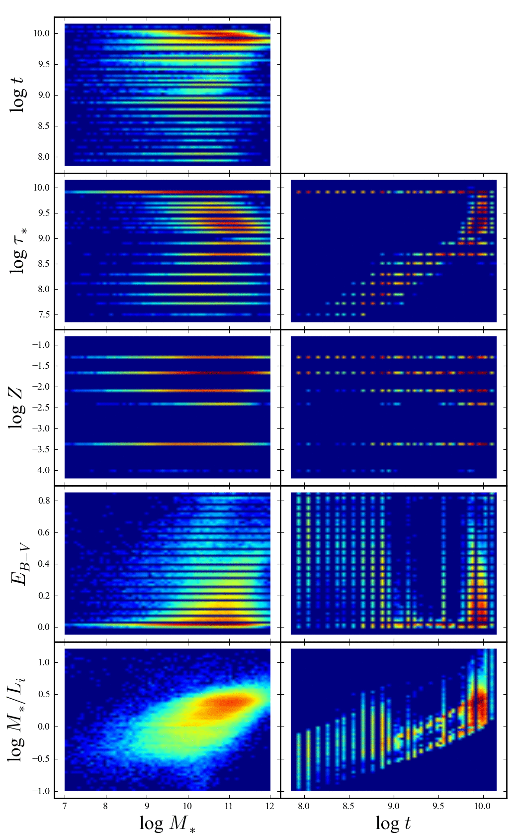
Figure 2: Why ‘best fit’ is not the best parameter estimator.— This Figure shows the distribution of parameter values corresponding to the single ‘best fit’ (i.e., maximum likelihood) template. The distributions shown in this Figure should be compared to the distributions of Bayesian estimators in Figure 3. It is immediately obvious how the use of a semi-regular grid of SP parameter values within our SPL produces strong discretisation in $t$, $\tau$, $Z$, and $\mathrm{E}_{B\text{-}V}$. In the lower-left panel, however, it can be seen that there is some quantisation in $M_{*}/L$, even though the distribution of $M_{*}/L$s in the SPL is more nearly continuous. As described in §3.4, this form of discretisation arises where there are strong degeneracies in the SPS fit that cannot be properly accounted for using a frequentist ‘best fit’ approach.

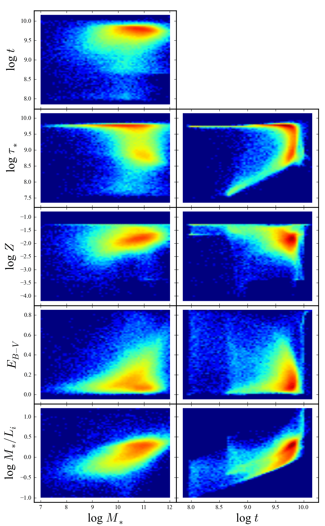
Figure 3: Illustrating the inferred distribution of SP parameters for GAMA galaxies.— In this Figure, we show the interrelationships between several important SP parameters for GAMA galaxies. Note that the SP library covers the full range of $t$, $\tau$, and $\mathrm{E}_{B\text{-}V}$ shown. The observed relations between these parameters shows that information about the process of galaxy formation and evolution can be extracted from galaxies’ SEDs. From an algorithmic point of view, the most important point to take from this plot is that by using a Bayesian approach, we are able for the most part to avoid ‘discretisation’ errors (i.e., preferred parameter values) associated with the use of a discrete grid of parameter values (cf. Figure 2). Further, note that particularly for $t$, $\tau$, and $Z$, these distributions are qualitatively different to those in Figure 2.

That said, this only works where several different parameter combinations provide an acceptable description of the data. If one particular template is strongly preferred—if the observational uncertainties in a galaxy’s SED are comparable to or less than the differences between the SEDs of different templates—then our approach reverts to a ‘best fit’, and we will again suffer from artificial quantisation in the fit parameters. For the same reasons, the formal uncertainty on the SP parameters will be artificially small in this case. Note that, somewhat perversely, this problem will become worse with increasing signal–to–noise. (See also Gallazzi & Bell, 2009, but note, too, that the inclusion of a moderate ‘systematic’ uncertainty in the observed SEDs works to protect against ‘single template’ fits.) In this sense, and in contrast to the quantisation in the ‘best fit’ values discussed above, quantisation in the Bayesian ‘most likely’ values does indicate inadequately fine sampling of the SPL parameter space. We have chosen our parameter grids with this limitation in mind; in particular, we have found that a rather fine sampling in the $\mathrm{E}_{B\text{-}V}$ dimension is required to avoid strong quantisation.

Although our SPL templates span a semi-regular grid in each of $t$, $\tau$, $Z$, and $\mathrm{E}_{B\text{-}V}$, the observed distribution in these parameters is anything but uniform. There is nothing in the calculation to preclude solutions with, for example, young ages and low metallicities. The fact that these regions of parameter space are sparsely- or un-populated shows that there are few or no galaxies with optical SEDs that are consistent with these properties. Figure 3 thus illustrates the mundane or crucial (depending on one’s perspective) fact that the derived SP parameters do indeed encode information about the formation and evolution of galaxies. It is particularly striking that there appears to be a rather tight and ‘bimodal’ relation between $t$ and $\tau$: there is a population of galaxies that are best fit by very long and nearly continuous SFHs ($\tau\approx 10$ Gyr), and another with $t/\tau\approx$ 3—10. There are virtually no galaxies inferred to have $t<\tau$.

The inferred distribution of parameter values is significant in terms of our assumed priors: it is clear that the derived parameter distributions do not follow our assumed priors (see also Figure 12). But this is not to say that the precise values are not more subtly affected by our particular choice of priors. In particular, the local slope of the priors on the scale of the formally derived uncertainties might act to skew the posterior PDF (see also Appendix A). In principle, it is possible to use the observed parameter distributions to derive new, astrophysically motivated priors. Then, if this were to significantly alter the observed parameter distribution, the process could be iterated until convergence. Such an exercise is beyond the scope of this work.

Next, in Figure 4, we show the distribution of inferred uncertainties in each of the parameters shown in Figure 3. As in Figure 3, there is some structure apparent in these distributions: the uncertainties in some derived properties are different for galaxies with different kinds of stellar populations. As a simple example, galaxies with $t\gg\tau$ have considerably larger uncertainties in $\tau$, as information about the SFH is washed out with the deaths of shorter-lived stars. In connection to the discretisation problem, the very young galaxies (seen in Figure 3 to suffer from discretisation in the values of $Z$) also have low formal values for $\Delta\log Z$ and/or $\Delta\log t$. But it is worth noting that in comparison to the uncertainties in other SP parameters, $\Delta\log M_{*}/L_{i}$ is more nearly constant across the population (this is perhaps more clearly apparent in Figure 5, described immediately below).

Our last task for this Section is to directly compare the frequentist ‘best fit’ and Bayesian ‘most likely’ SP values; this comparison is shown in Figure 5 . In each panel of this Figure, the ‘$\Delta$’ plotted on the $y$ axis should be understood as being the ‘best fit’-minus-‘most likely’ value; these are plotted as a function of the Bayesian estimator. Within each panel, the dashed white curves show the median $\pm 3\sigma$ uncertainty in the $y$-axis quantity, derived in the Bayesian way, and computed in narrow bins of the $x$-axis quantity. These curves can thus be taken to indicate the formal consistency between the best fit and most likely parameter values.

In practice, there is an appreciable systematic difference between the frequentist and Bayesian parameter estimates. In general, we find that traditional, frequentist estimates are slightly older (by $\approx 0.14$ dex), less dusty (by $\approx 0.07$ mag), and more massive (by $0.09$ dex) than the Bayesian values. In comparison to the formal uncertainties, these systematic differences are at the 0.5—0.7$\sigma$ level; this is despite the fact that the ‘best fit’ value is within 1.5$\sigma$ of the ‘most likely’ value for 99 % of objects. And again, we stress that, formally, the Bayesian estimator is the correct value to use.

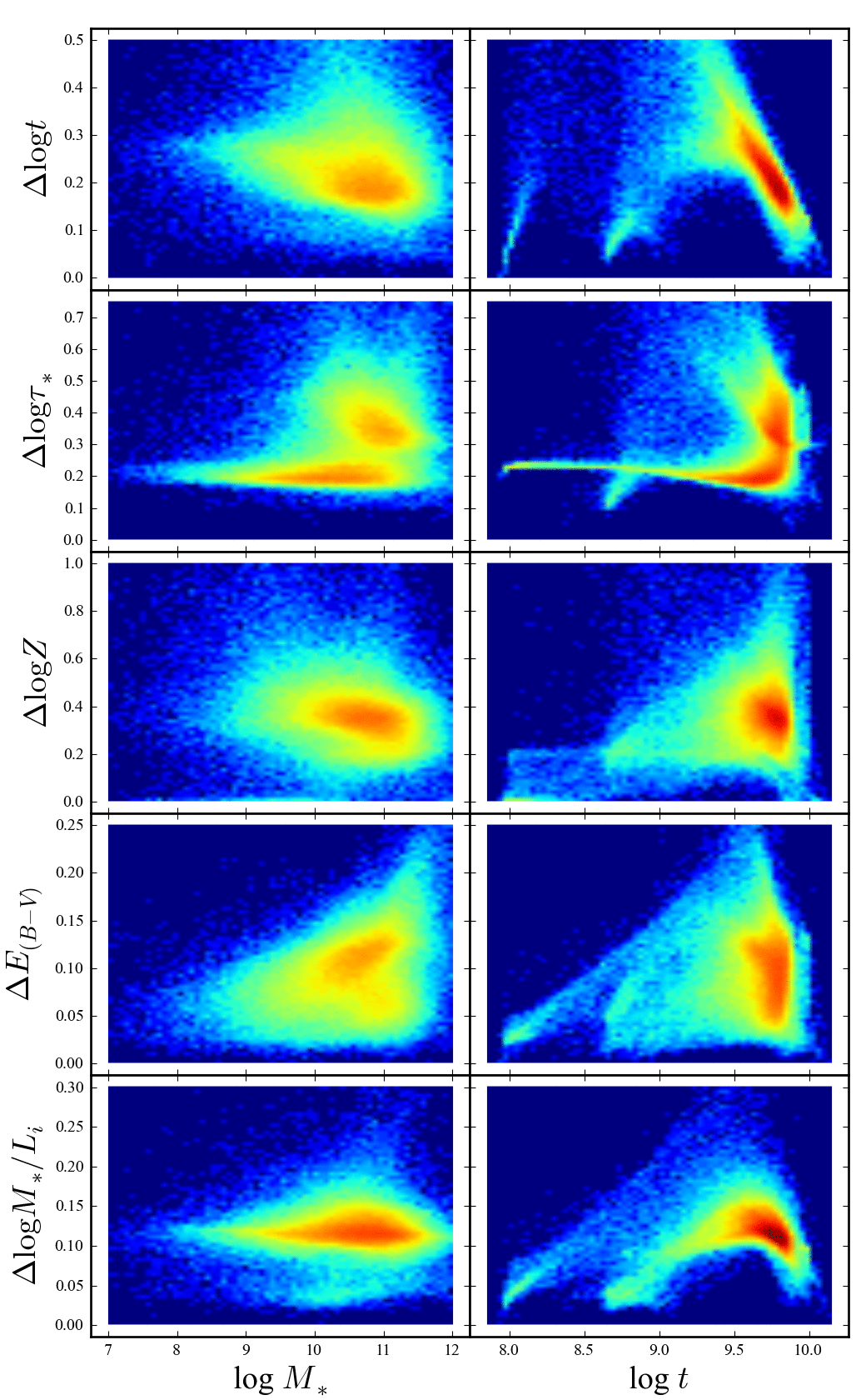
Figure 4: Illustrating the distribution of parameter uncertainties.— In this Figure, we show the formal uncertainties for several important parameters. The structure that is apparent in the different panels of this plot shows that our ability to constrain $t$, $\tau$, and $Z$ is different for different stellar populations. The crucial point to be made from this Figure, however, is that the formal uncertainty in $M_{*}/L_{i}$ is $\approx 0.1$ dex for the vast majority of galaxies, with essentially no dependence on the uncertainties in other parameter values.

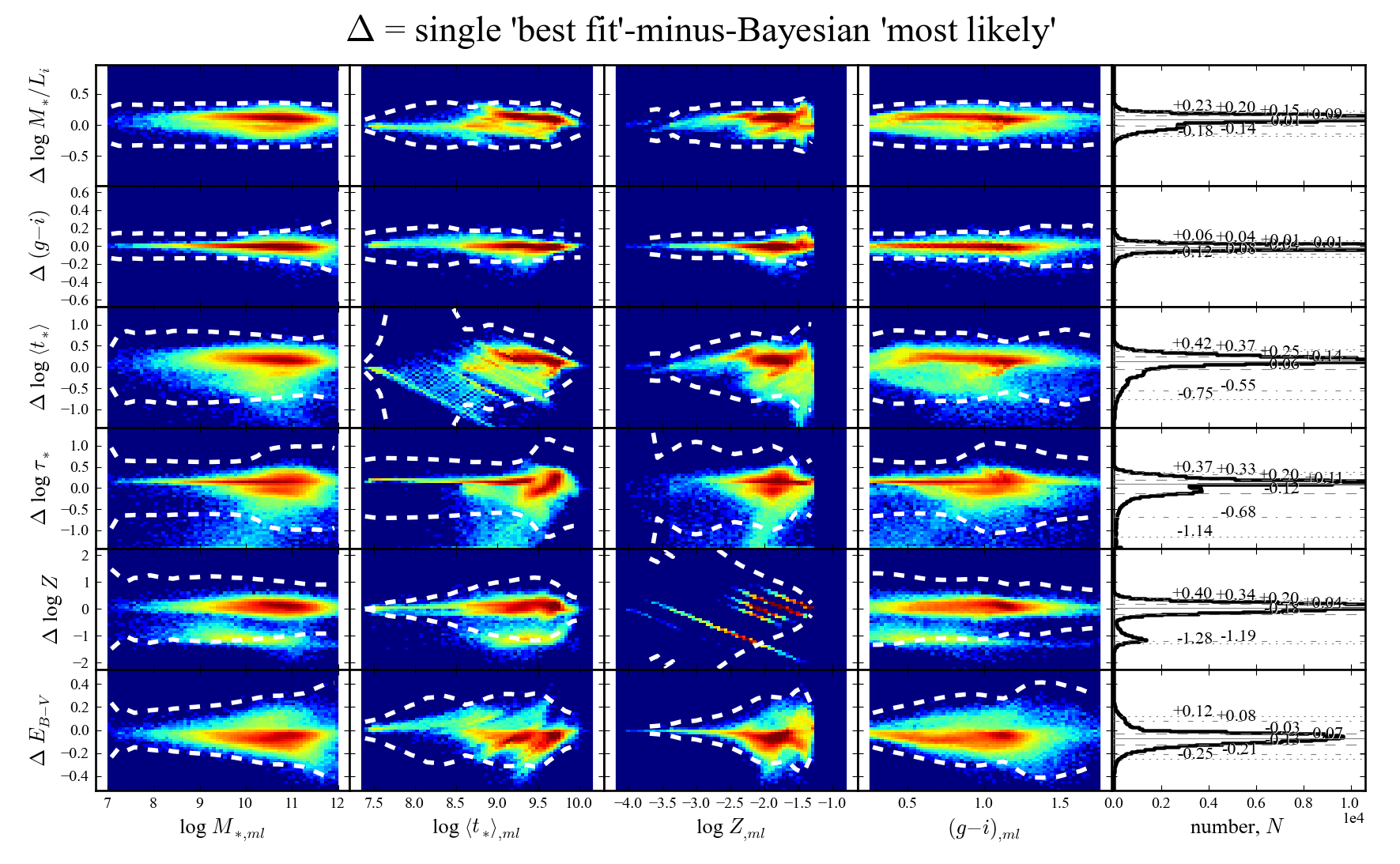
Figure 5: Using a frequentist ‘best fit’ estimator leads to significant biases in the inferred SP parameter values.— In this Figure, we show the difference between the ‘best fit’ (i.e., maximum likelihood) value, and the Bayesian ‘most likely’ value of a number of key parameters. The ‘$\Delta$’ plotted on the $y$ axis should be understood as being the ‘best fit’–minus–‘most likely’ value. Strong quantisation in the ‘best fit’ values can be clearly seen for $\left<t_{*}\right>$ and particularly $Z$. Further, in the right-hand panels of this Figure, we look at the random and systematic differences between these two parameter estimates; the numbers in each panel show the equivalent of the $0$, $\pm 1$, $\pm 2$, and $\pm 3\sigma$ percentiles for each distribution. In particular, note that the ‘best fit’ (which again we stress is not the correct estimator to use) value of $M_{*}/L$ is systematically higher than the ‘most likely’ value by 0.09 dex.

As a final aside for this section, we note that the importance of Bayesian analysis has been recognised in the context of photometric redshift evaluation (a problem which is very closely linked to SPS fitting) by a number of authors, including Benitez (2000) and Brammer et al. (2008). While most of the SPS fitting results for SDSS (e.g. Kauffmann et al., 2003b; Brinchmann et al., 2004; Gallazzi et al., 2005) have been based on a Bayesian approach, it is still common practice to derive SPS parameter estimates using simple $\chi^{2}$ minimisation (Walcher et al., 2011). This is particularly true for high redshift studies (but see Pozetti et al., 2007; Walcher et al., 2008).

3.5 Detection/selection limits and $\mathbf{1/V_{\mathrm{max}}}$ corrections

GAMA is a flux-limited survey. For a number of science applications—most obviously measurement of the mass or luminosity functions—it is important to know the redshift range over which an individual galaxy would be selected as a spectroscopic target. To this end, we have used the SP fits described above to determine the maximum redshift, $z_{\mathrm{max}}$, at which each galaxy in the GAMA catalogue would satisfy the main GAMA target selection criterion of $r_{\mathtt{petro}}<19.4$, or, for the G12 field, $r_{\mathtt{petro}}<19.8$. (Recall that the target selection is done on the basis of the SDSS, rather than the GAMA, petro magnitude.)

This has been done for each galaxy using the best-fit template spectrum. Knowing the best-fit template, including the normalisation factor, $A_{T}$, we consider how the observers’ frame $r$-band flux of the template declines with redshift. Knowing that galaxy’s observed $r_{\mathtt{petro}}$, it is then straightforward to determine the redshift at which the observers’ frame $r$-band flux drops to the appropriate limiting magnitude. The only complication here is accounting for both the cosmological redshift and the Doppler redshift due to peculiar velocity in the redshift. This is done by recognising that $(1+z_{\mathrm{helio}})=(1+z_{\mathrm{dist}})(1+z_{\mathrm{pec}})$; the values of $z_{\mathrm{max}}$ should be taken as pertaining to $z_{\mathrm{dist}}$.

In Figure 6, we use the value of $z_{\mathrm{max}}$, so derived, to show GAMA’s stellar mass completeness limit expressed as a function of redshift and restframe colour. This Figure shows the two-fold power of GAMA in relation to SDSS. First, for dwarf galaxies, GAMA is $\approx 95$ % complete for $M_{*}\approx 10^{8}$ M_⊙ and $z\approx 0.05$; at these masses, SDSS completeness is $\lesssim 80$ % even for $z<0.02$. GAMA thus provides the first census of $10^{7.5}<M_{*}<10^{8.5}$ M_⊙ galaxies. Further, for massive galaxies, GAMA probes considerably higher redshifts: for $M_{*}\sim 10^{10.5}$ ($10^{11}$) M_⊙, where SDSS is limited to $z\lesssim 0.1$ (0.15), GAMA can probe out to $z\approx 0.25$ (0.3). Said another way, GAMA probes roughly twice the range of lookback times of SDSS. GAMA thus opens a new window on the recent evolution of the massive galaxy population.

In the right-hand panel of Figure 6, we show these same results in complementary way. The solid lines in this Figure show the mean value of $z_{\mathrm{max}}$ as a function of $M_{*}$ and restframe $(g-i)$. These values are for the main $r_{\mathtt{petro}}<19.4$ selection only; for the G12 field, these limits should be shifted down in mass by 0.16 dex.

In this panel, for comparison, we also show the incompleteness-corrected bivariate colour-mass distribution for $z<0.12$ galaxies; i.e., individual galaxies have been weighted by $1/V_{\mathrm{max}}$, where $V_{\mathrm{max}}$ is the survey volume implied by $z_{\mathrm{max}}$. Note that in the construction of this plot, we have only included galaxies with a relative weight $<30$ (i.e., $z_{\mathrm{max}}>0.0375$); in effect, this means that we have not fully accounted for incompleteness for $M_{*}\lesssim 10^{8}$ M_⊙. Again, we see that GAMA probes the bulk of the massive galaxy population ($M_{*}\gtrsim 10^{10.5}$ M_⊙) out to $z\approx 0.25$.

Before moving on, we make two further observations. First, it is clear that the red sequence galaxy population extends well below the ‘threshold mass’ of $10^{10.5}$ M_⊙ suggested by Kauffmann et al. (2003b). Secondly, it appears that we are seeing the low-mass end of the red sequence population: the apparent dearth of galaxies with $(g-i)\gtrsim 0.8$ and $10^{8.5}\lesssim M_{*}/$M_⊙ $\lesssim 9.5$ is not a product of incompleteness. We will investigate these results further in a future work.

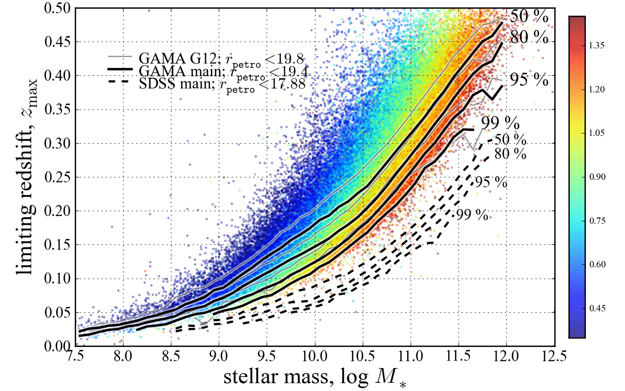
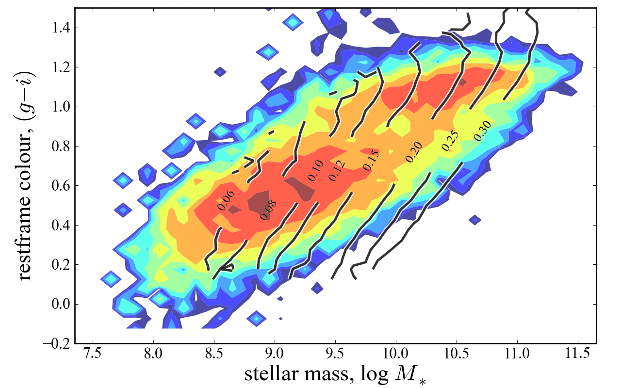
Figure 6: The GAMA stellar mass completeness limits as a function of redshift and restframe colour.— Both panels of this plot use the derived values of $z_{\mathrm{max}}$ (that is, the maximum redshift at which any individual galaxy would satisfy the $r$-band selection limit) to show the redshift-dependent GAMA completeness limit as a function of stellar mass and restframe colour. In the left panel, we show the stellar mass for which GAMA is 50/80/95/99 % complete, computed in narrow bins of $z_{\mathrm{max}}$. The heavier solid lines show the completeness for the main $r_{\mathtt{petro}}<19.4$ GAMA selection limit; the lighter solid lines show that for the deeper $r_{\mathtt{petro}}<19.8$ limit for the G12 field; the dashed lines show the completeness for the SDSS $r_{\mathtt{petro}}<17.88$ main galaxy sample selection limit. In this panel, individual plots are colour-coded according to their restframe $(g-i)$ colour; only galaxies from the main $r_{\mathtt{petro}}<19.4$ sample are shown. In the right panel, the black contours show the mean value of $z_{\mathrm{max}}$, again for the main $r_{\mathtt{petro}}<19.4$ sample, projected onto the colour–stellar mass diagram. For comparison, the filled, coloured contours in this panel show the incompleteness corrected bivariate colour–stellar mass distribution of $z<0.12$ galaxies; these contours are logarithmically spaced by factors of 2. In constructing this plot, individual galaxies have been weighted by $w=V(z=0.12)/V(z_{\mathrm{max}})$. We have only counted galaxies with a relative weighting $w<30$. In effect, this means that we have not fully corrected for incompleteness for $z_{\mathrm{max}}<0.04$ or $M_{*}\lesssim 10^{8.5}$ M_⊙.

4 How much does NIR data help (or hurt)?

Conventional wisdom says that that using NIR data leads to a better estimate of stellar mass. The principal justification for this belief is that, in comparison to optical wavelengths, and all else being equal, NIR luminosities 1. vary less with time, 2. depend less on the precise SFH, and 3. are less affected by dust extinction/obscuration. Further, whereas old stellar populations can have very similar optical SED shapes to younger and dustier ones (see Figure 1), the optical–NIR SED shapes of these two populations are rather different. The inclusion of NIR data can thus break the degeneracy between these two qualitatively different situations, and so provide tighter constraints on each of age, dust, and metallicity—and hence, it is argued, a better estimate of $M_{*}/L$.

There are, however, several reasons to be suspicious of this belief. First, while stellar evolution models have been well tested in the optical regime, there is still some controversy over their applicability in the NIR. This has been most widely studied and discussed recently in connection with TP-AGBs stars in the models of BC03 and M05 (e.g., Maraston, 2006; Bruzual, 2007; Kriek et al., 2010). The different models have been shown to yield stellar mass estimates that vary by as much as $\sim 0.15$ dex for some individual galaxies (e.g., Kannappan & Gawiser, 2007; Wuyts et al., 2009; Muzzin et al., 2009), but only if restframe NIR data are used in the fits.

Separately from the question as to the accuracy of SP models in the NIR, there are a number of empirical arguments suggesting that optical data alone can be used to obtain a robust and reliable stellar mass estimate. A number of authors have found that there is a remarkably tight relation between optical colour and stellar mass-to-light ratio (Bell & de Jong, 2001; Bell et al., 2003; Zibetti et al., 2009; Taylor et al., 2010a). As described in §1.2, Gallazzi & Bell (2009) have argued that a stellar mass estimate based on a single colour is nearly as reliable and robust as one based on a full optical–to–NIR SED fit, or even one based on spectral diagnostics. Further, using their NMF-based kcorrect algorithm that eliminates the need for assuming parametric SFHs, Blanton & Roweis (2007) have shown that they are able to use optical SEDs to predict galaxies’ NIR fluxes. Each of these results implies that the NIR SED does not, in practice, contain qualitatively ‘new’ information not found in the optical.

With this as background, our goal in this Section is to examine how the inclusion of NIR data affects our stellar mass estimates. We will take an empirical approach to the problem, looking at how both the quality of the fits and the quantitative results themselves depend on the models and photometric bands used. We will argue that, at least at the present time, the NIR data cannot be satisfactorily incorporated into our SPS fitting. We explore the possible causes of our problems in dealing with the NIR SEDs to §4.4. In the next Section, we will then look at whether and how our decision to ignore the NIR data affects the quality of our stellar mass and SP parameter estimates.

4.1 How well do the models describe the optical-to-NIR SEDs of GAMA galaxies?

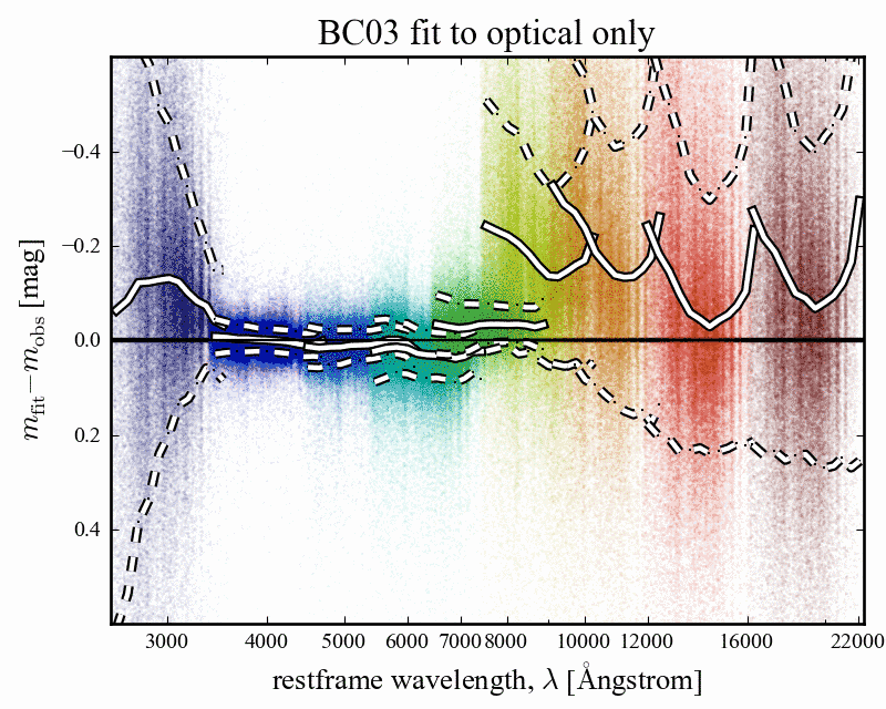
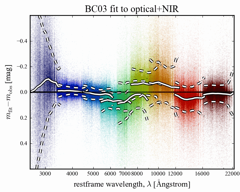
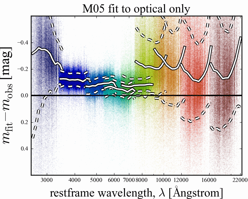
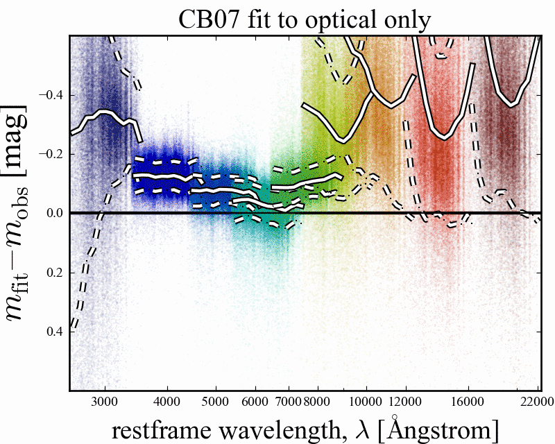
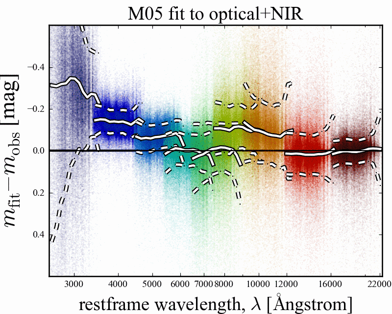
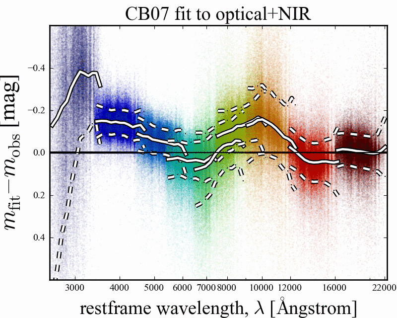
Figure 7: Illustrating how well the models describe the observed photometry of real galaxies.— Each panel of this Figure shows the residuals when fitting either to the optical $ugriz$ (left panels) or the full $ugrizYJHK$ (right panels) SEDs. The main upper panels are for fits based on the BC03 stellar evolution models; the lower panels show the same using the M05 or CB07 models. Within each panel, the different colours refer to the different observed bands. For each band the white lines show the median (solid lines) and 16/84 percentile (dashed lines) residual in each band as a function of restframe wavelength or, equivalently, redshift. This Figure should be compared to Figure 16. From the left-hand panels, it is clear that all three of these SPS models provide an acceptable description of the optical SEDs, with relatively small residuals as a function of restframe wavelength. That said, these optical-only fits overpredict the NIR fluxes by $\sim 0.2$ dex. In the righthand panels, it can be seen that including the NIR data significantly degrades the quality of the optical fits, particularly in the $i$- and $z$-bands. Each of the three sets of models show qualitatively and quantitatively similar residuals: while each set of models yield similarly good fits to the optical data alone, none of these models provides a good description of the optical–to–NIR SEDs of GAMA galaxies. Based on our experiences with mock galaxy photometry in Appendix A, these results suggest strong inconsistencies between the optical–minus–NIR colours of real galaxies and those contained within our SPL.

In Figure 7, we show the residuals from the SED fits as a function of restframe wavelength; i.e., $m_{X,\mathrm{fit}}-m_{X,\mathrm{obs}}$ as a function of $\lambda_{X}/(1+z)$. Figure 7 should be compared to Figure 16 in Appendix A. This Appendix describes how we have applied our SPS fitting algorithm to mock galaxy photometry, which we have constructed from the fits to the actual $ugriz$ SEDs of GAMA galaxies. In this way, as in Gallazzi & Bell (2009), we have tested our ability to fit galaxy SEDs in the case that the SPL provides perfect descriptions of the stellar populations of ‘real’ galaxies, and that the data are perfectly calibrated (i.e., no systematics in the photometric cross-calibration). Inasmuch as they can inform our expectations for the real data, the results of these numerical experiments (shown in Figure 16) can help interpret the offsets seen in Figure 7.

In Figure 7, as in Figure 16, the lefthand panels show the residuals when only the optical data is used for the fit. The NIR points in these panels are thus predictions for the observers’ frame NIR photometry derived from the optical SED. The right-hand panels of both Figures 7 and 16 show the residuals for fits to the full 9 band optical–to–NIR SED. In Figure 7, we show the residuals when using several different sets of SSP models to construct our SPL. In this Figure, the larger upper panels are for the fits based on the BC03 SSP models; the panels below show the same using the SSP models of M05 and CB07 for comparison.

Looking first at the lefthand panels of Figure 7, we see that our SPS fits provide a reasonably good description of the observed $ugriz$ SEDs of real GAMA galaxies. The fit residuals are qualitatively and quantitatively similar when using each of the three different SSP models to construct the SPL. The median offset in each of the $(ugriz)$-bands is $\approx$ ($-$0.10, $-$0.00, +0.01, +0.02, $-$0.03) mag. In terms of the formal uncertainties from the fits, the median offsets are at the level of $\approx$ ($-$0.3, $-$0.0, +0.2, +0.5, $-$0.5)$\sigma$. The systematic biases in the fit photometry are thus weakly significant, but, at least for the $griz$-bands, well within the imposed error floor of 0.05 mag.

How does this compare to what is seen for the mocks in Figures 16? We find qualitatively similar offsets when fitting to the mock $ugriz$ photometry. More specifically, we see a similar ‘curvature’ in the residuals, with slight excesses in the fit values for the $u$- and $z$-band photometry, and the $gri$- band photometry being very slightly too faint. It is true that, quantitatively, the offsets seen in Figure 7 are about twice as large as we might expect based on our numerical experiments ($\lesssim 0.5\sigma$ for the real data, as opposed to $\lesssim 0.2\sigma$ for the mocks). But even so, the fact that we see similar residuals when fitting to the mocks shows that such residuals are to be expected, even in the ideal case where both the SPL and photometry are perfect. We do not, therefore, consider the mild systematic offsets between the fit and observed photometry as evidence for major problems in the $ugriz$ fits.

Unlike Blanton & Roweis (2007), we seem unable to use the optical SEDs to satisfactorily predict NIR photometry. The fits to the $ugriz$ data predict $YJHK$ photometry that is considerably brighter (by up to $\sim 0.2$ mag) than what is observed. The systematic differences between the predicted and observed fluxes for the BC03 models are $-3.3\sigma$ $-2.8\sigma$, $-1.6\sigma$, and $-2.5\sigma$ in $YJHK$, respectively. For the M05 models, the residuals are slightly larger ($-3.3\sigma$, $-3.0\sigma$, $-2.3\sigma$, and $-2.8\sigma$), and larger again for the CB07 models ($-4.7\sigma$, $-5.6\sigma$, $-6.0\sigma,$ and $-8.2\sigma$).

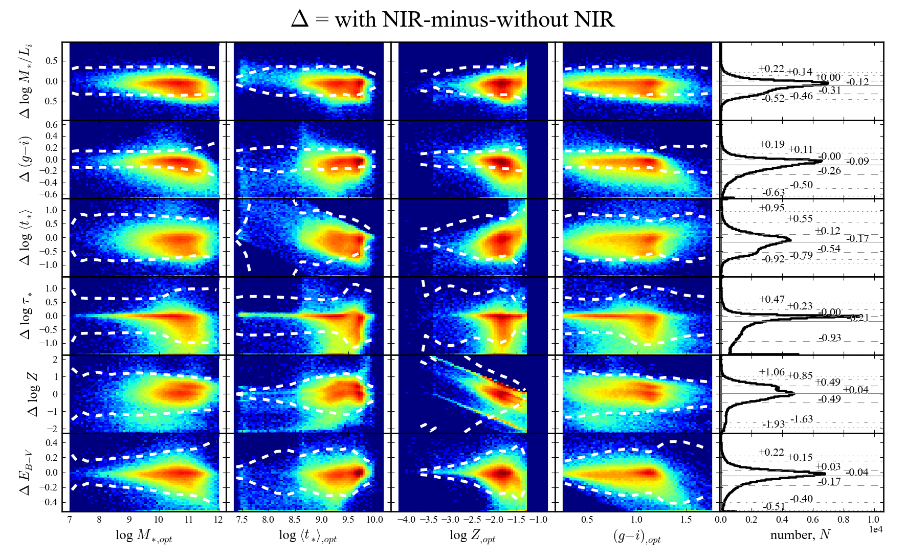
Figure 8: The effect of including the NIR data on the inferred stellar population parameters.— In each panel of this Figure, we show the difference between the stellar population parameters derived using only the $ugriz$ photometry, and those derived using the full $ugrizYJHK$ SEDs. In all cases, the ‘$\Delta$’ should be understood as ‘optical-plus-NIR-derived’–minus–‘optical-only-derived’. As in Figure 5, the histograms in the right-hand panels show the distribution of ‘$\Delta$s’ and the 1/2.5/15/50/85/97.5/99 percentiles. In the other panels, the ‘$\Delta$’ is plotted as a function of the ‘optical-only-derived’ value; the colourscale shows the logarithmic data density for the full GAMA sample. In these panels, the dashed lines show the $\pm 3\sigma$ uncertainties as derived from the fits to the 5 optical bands. The median effect of including the NIR data is to systematically reduce the inferred value of $M_{*}$ by $\approx 0.1$ dex. It is important to note these offsets NIR-derived values are formally inconsistent with the optical-only-derived uncertainties at the $\gtrsim 2.5\sigma$ level. This is particularly significant in the case of the restframe $(g-i)$ colour (median $\Delta(g-i)=0.1$ mag), which should be independent of the NIR data. Coupled with the fact that the models do not provide a satisfactory description of the observed SEDs (see Figure 7), we are thus obliged to consider the NIR-derived SP parameters as suspect.

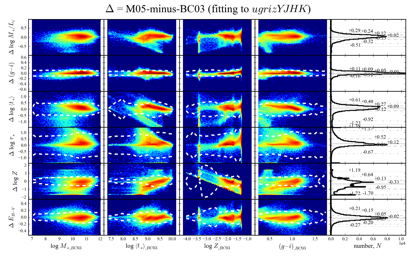
Figure 9: Comparison between M05- and BC03-based parameter estimates, derived from fits to the $ugrizYJHK$ SEDs.— The ‘$\Delta$’s in this Figure should be understood as the M05-based-minus-BC03-based parameter values; all symbols and their meanings are analogous to Figure 8. While, as expected, there are some systematics in the inferred values of $M_{*}$ as a function of $\left<t_{*}\right>$, the global agreement is very good. In comparison to Figure 8, the systematic differences between parameters derived on the basis of the different stellar evolution models (but the same $ugrizYJHK$ data) are considerably larger than the differences between the values inferred with or without the inclusion of the NIR data (but the same stellar evolution models). This suggests that our apparent inability to adequately fit the observed optical-to-NIR SED shapes of GAMA galaxies is not a product of errors in the stellar evolution models. At the same time, however, the ‘random’ differences between the M05- and BC03-based SP parameter estimates are larger than the formal uncertainties when the NIR data are included. This is not true when using only the optical data. That is, the model dependence of the SP parameter estimates becomes significant if, and only if, the NIR data are included.

The fits to the mock galaxies’ optical SEDs also over-predict the ‘true’ NIR fluxes, but, as can be seen in Figure 16, in a qualitatively different way to what we see for real galaxies. In the case of the mock galaxies, the offset between the predicted and actual NIR fluxes is a much smoother function of rest-frame wavelength, as might be expected from simple extrapolation errors. This is in contrast to the sharp discontinuity in the residuals seen in Figure 7 between the optical and NIR bands.

Looking now at the righthand panels of Figure 7, we see that none of the three stellar population libraries are able to satisfactorily reproduce the optical–NIR SED shapes of GAMA galaxies without significant systematic biases. Each of the models shows a significant excess of flux for 7000 Å$\lesssim\lambda\lesssim$ 12000 Å. The significance of the offsets in the $i$-, $Y$-, and $J$-bands are $\sim+1.8\sigma$, $-1.6\sigma$, and $-1.4\sigma$, respectively. Based on our numerical experiments, there is no reason to suspect that we should be unable to reproduce the observed optical–to–NIR SED shapes of real galaxies. As can be seen in Figure 16, the fits to the mock $ugrizYJHK$ SEDs are near perfect.

Each of the issues highlighted above point to inconsistencies between the optical–to–NIR colours of our SPL models on the one hand, and of real galaxies on the other. Further, the fact that the models fail to satisfactorily describe the NIR data immediately calls into question the reliability of parameter estimates derived from fits to the full optical-to-NIR photometry. The rest of this section is devoted to exploring the nature of this problem.

4.2 How including NIR data changes the parameter estimates

Figure 8 shows the difference between stellar population parameters derived from the $ugriz$ and the $ugrizYJHK$ photometry, and using the BC03 models to construct our stellar population library as per §3.2. In this Figure, the ‘$\Delta$’s plotted on the $y$-axis should be understood as the 9-band–minus–5-band-derived value; these offsets are plotted as a function of the 5-band-derived value.

In the simplest possible terms, the 9-band fits yield systematically lower values for all of $M_{*}$, $M_{*}/L_{i}$, $\mathrm{E}_{B\text{-}V}$, $\left<t_{*}\right>$, and $(g-i)$ than the 5-band fits. Again, based on our experiences with the mock catalogues described in Appendix A, we have no reasons to expect these sort of discrepancies: for the mocks, we are able to recover the input SP parameters with virtually no systematic bias using either the optical–only or optical–plus–NIR SEDs (see Figure 17).

In each case, based on the formal uncertainties from the 5-band fits, the median significance of the offset in the SP parameter estimates is $\gtrsim 1.5\sigma$. For each of these quantities, the 9-band-derived value is formally inconsistent with the 5-band-derived value at the $>3\sigma$ level for $\approx$ 25 % of galaxies. (Using the M05 models, we find a similar fraction; using the CB07 models, this fraction goes up to 30–40 %.) This shows that the residuals seen in Figure 7 are more than merely a cosmetic problem—they are symptomatic of inconsistencies between the fits with and without the inclusion of the NIR.

To make plain the importance of these systematic offsets, consider the fact that there are large and statistically significant differences in the $(g-i)$ colours inferred from the 9-band and 5-band fits. The median values inferred from the fits with the NIR included are 0.10 mag bluer than those based on the optical alone. In comparison to the formal uncertainties in the 5-band derived values of $(g-i)$, this amounts to an inconsistency at the $\sim 2.5\sigma$ level. And this is despite the fact that the NIR data by definition contain no information about $(g-i)$. Looking at Figure 7, it is clear that the 5-band fits are a more reliable means of inferring a restframe $(g-i)$ colour: for the 9-band fits, the differential offset between the $g$ and $i$ bands is $\approx 0.10$ mag; for the 5-band fits, the differential offset is $\lesssim 0.03$ mag.

Said another way, because the 9-band fits have the wrong SED shape, they cannot be used to infer a restframe colour. But the same is true of any other derived property—simply put, if the models cannot fit the data, they cannot be used to interpret them.

4.3 The sensitivity of different SSP models to the inclusion/exclusion of NIR data

One possible explanation for the large residuals seen in Figure 8 is problems with the BC03 SSP models. In particular, one might worry that these are related to the NIR contributions of TP-AGB stars. In this context, let us begin by noting that if this were to be the source of the problems that we are seeing, then we would expect the optical–only fits to underpredict the ‘true’ NIR fluxes, particularly for the BC03 models. But this is not what we see: the optical–only fits overpredict galaxies’ NIR fluxes using both the BC03 and the M05 models, and by similar amounts in both cases.

In Figure 9, we show the comparison between the M05 - and BC03 -derived SP parameter values, based on fits to the full $ugrizYJHK$ SEDs. It is clear from Figure 9 that there are systematic differences between the models, particularly (and as expected) for $\left<t_{*}\right>\sim 10^{8.5}$—$10^{9.5}$ Gyr.

Taking an empirical perspective on the problem, we can consider these differences as an indication of the degree of uncertainty tied to uncertainties in the stellar evolution tracks that underpin the SSP spectra. Using only the optical data, the systematic differences between any of the SP parameter values derived using the different models is small: for $M_{*}/L_{i}$, the median offset is 0.01 dex. That is, when using optical data only, these famously ‘disagreeing’ models yield completely consistent results. This is in marked contrast to a number of results emphasising the importance of differences in the modelling of TP-AGB stars in the BC03 and M05 models when NIR data are used (e.g. Cimatti et al., 2008; Wuyts et al., 2009). In terms of ‘random’ differences, the inferred values of $M_{*}$ based on the two sets of models agree to within $\pm 0.3$ dex (a factor of 2) for 99 % of galaxies. We can treat the 15/85 percentile points of the distribution of the ‘$\Delta$’s as indicative of the 1$\sigma$ random ‘error’ associated with the choice of SSP model. For $M_{*}/L$, this ‘error’ is $\lesssim 0.10$ dex. That is, when using only optical data, the SP parameter estimates are not significantly model dependent.

When we include the NIR data in the fits, the agreement between the SP values inferred using the two different sets of SSP models is not as good. The inferred values of $M_{*}$ using the BC03 or M05 models agree to within $\pm 0.5$ dex (a factor of 3) for 99 % of galaxies; the 1$\sigma$ random ‘error’ in $M_{*}$ is $\approx 0.12$ dex. While the inferred values of $M_{*}/L$ agree reasonably well, the differences in the other inferred stellar population parameters— $\mathrm{E}_{B\text{-}V}$, $Z$, and especially $\left<t_{*}\right>$—are larger. For $\left<t_{*}\right>$, the $1\sigma$ ‘error’ is $\approx 0.3$ dex; this should be compared to the formal uncertainty in $\left<t_{*}\right>$ of $\sim 0.2$ dex. Thus we see that the ‘error’ in SP parameter estimates associated with the choice of model becomes comparable to the formal uncertainties when, and only when, NIR data is included in the fit.

4.4 What is the problem with the NIR?

What can have possibly gone wrong in the fits to the NIR data? There are (at least) three potential explanations for our inability to obtain a good description of the optical–NIR SED shapes of GAMA galaxies using the models in our SPL. The first is problems in the data. The second is problems in the stellar evolution models used to derive the SSP spectra that form the basis of our template library. The third is problems in how we have used these SSP spectra to construct the CSPs that comprise our SPL.

4.4.1 Is the problem in the data? Maybe.

We cannot unambiguously exclude the possibility of errors in, for example, the basic photometric calibration of the NIR imaging data. In this context, we highlight the qualitative difference in our ability to use optical data to predict NIR fluxes for the real GAMA galaxies on the one hand, and for mock galaxies on the other. In particular, the sharp discontinuity in the residuals between the $z$- and $Y$-bands for the real galaxies would seem to suggest a large inconsistency between these two bands at the level of $\sim 0.1$–$0.2$ mag.

As described in §2.2, GAMA has received the NIR data fully reduced and calibrated. In order to ensure that there are not problems in our NIR photometric methods (which are not different from those in the optical), we have verified that there are no large systematic offsets between our photometry and that produced by CASU. This would suggest that any inconsistencies would really have to be in the imaging data themselves.

The accuracy of the UKIRT WFCAM data calibration has been investigated by Hodgkin et al. (2009) through comparison to sources from the 2MASS point source catalogue (Cutri et al., 2003; Skrutskie et al., 2006): they argue that the absolute calibrations of the $Y$- and $JHK$-band are good to $\sim 2$ and $\sim 1.5$ %, respectively. Taken at face value, this argues against there being such large inconsistencies in the photometry.

In light of the fact that we have not been directly involved in the reduction or calibration of these data, and with the anticipated availability of the considerably deeper VISTA-VIKING NIR imaging in the near future, we will not investigate this further here.

4.4.2 Is the problem in the SSP models? Probably not.

From what we have already seen, we can exclude errors in the SSP models as a likely candidate. We have shown in Figure 7 that none of the BC03 , M05 , or CB07 models provides a good description of the full optical-to-NIR SEDs of real galaxies—these models all show qualitatively and quantitatively similar fit residuals. Taken together, the results in Figures 8 and 9 show that (for the same data) the SP parameters derived using different models show small systematic differences, while at the same time (for any given set of SSP models) there is a large systematic difference between the values derived with or without the NIR data. This is not to say that the models are perfect, but the offsets seen in Figure 7 would appear to be larger than can be explained by uncertainties inherent in the SSP models themselves.

4.4.3 Is the problem in the construction of the SPL? Probably.

This leaves the third possibility that the assumptions that we have made in constructing our SPL are overly simplistic, in the sense that they do not faithfully describe or encapsulate the true mix of SPs found in real galaxies. We defer discussion of this possibility to §6.2. For now, however, we stress that the present SPL does seem to be capable of describing the optical SED shapes of real galaxies.

4.5 Summary—why the NIR (currently) does more harm than good

We have now outlined three reasons to suspect that, at least in our case, SP parameter estimates based only on optical photometry are more robust than if we were to include the NIR data:

1. Regardless of which set of SSP models we use, we see much larger than expected residuals in the SED fits when the NIR data are included. If the models do not provide a good description of the data, then we cannot confidently use them to infer galaxies’ SP properties.

2. The consistency between the SP parameter estimates derived with or without the inclusion of the NIR data is poor. For a sizeable fraction of GAMA galaxies ($\gtrsim 25$ %), the SP parameter values inferred from fits to the optical–plus–NIR SEDs are statistically inconsistent (at the $3\sigma$ level) with those based on the optical alone.

3. When using different models to construct the SPL templates, the agreement between the derived SP parameters is very good when the NIR data are excluded, but considerably worse when the NIR data are included. That is, the fit results become significantly model-dependent when, and only when, we try to include the NIR data.

For these reasons, and for the time being, we choose not to use the NIR data when deriving the stellar mass estimates. This begs the question as to how accurately $M_{*}/L$ can be constrained based on optical data alone, which is the subject of the next Section.

5 The theoretical and empirical relations between $\mathbf{M_{*}/L}$ and colour

As we have said at the beginning of §4, conventional wisdom says that NIR data provides a better estimate of stellar mass. Our conclusion in §4, however, is that we are unable to satisfactorily incorporate the NIR data into the SPS calculation. With this as our motivation, we will now look at how well $M_{*}/L$ can be constrained on the basis of optical data alone. In particular, we want to know whether or to what extent the accuracy of our stellar mass estimates is compromised by our decision to ignore the NIR data.

5.1 Variations in $\mathbf{M_{*}/L}$ at different wavelengths

Part of the rationale behind the idea that the NIR provides a better estimate of $M_{*}/L$ is that galaxies show less variation in their NIR $M_{*}/L$s than they do in the optical. We address this issue in Figure 10; this Figure merits some discussion. Each panel of Figure 10 shows a subsample of the models in our SPL. Within each panel, models are colour-coded according to their metallicity (from the lowest metallicity in blue to the highest metallicity in red). For each metallicity, the slightly heavier line shows how the single burst (i.e., $\tau\rightarrow 0$) track evolves with time, $t$; the other single-colour lines then connect models with the same age (but different $\tau$s) or the same SFH $e$-folding time (but different ages). Finally, the colour-graded lines connect models with the same $t$ and $\tau$, but different metallicities. In this way, each panel shows a 2D projection of the 3D ($t$, $\tau$, $Z$) grid of SPL templates. Note that we only show zero-dust models in this Figure; the dust-extinction vector is shown in the lower-right corner of each panel.

Each row of Figure 10 shows the mass–to–light ratio in different bands ($uiJK$, from top to bottom). Let us look first at the first column, in which we plot each of these $M_{*}/L$s as a function of time. For fixed $Z$ and $\tau$, and particularly for $t\gtrsim 2$ Gyr, it is true that the NIR $M_{*}/L$ varies less with $t$ than does the optical $M_{*}/L$—but not by all that much. For the SSP models, the total variation in $M_{*}/L$ between 2 and 10 Gyr is $\lesssim 1.2$ dex in the $u$ band, compared to $\lesssim 0.7$ dex in the $i$-band, and $\approx 0.6$ dex in the $J$- and $K$-bands. Similarly, it is also true that at fixed $t$ and $Z$, the spread in $M_{*}/L$s for different $\tau$s is slightly smaller for longer wavelengths: the total variation goes from $\lesssim 1.2$ dex in the $g$-band to $\lesssim 0.4$ dex in the $i$-band, to $\lesssim 0.3$ dex in the $J$- and $K$-bands. Considering variations in $M_{*}/L$ with all of $t$, $\tau$, and $Z$, the full range of $M_{*}/L$s becomes 2.7, 1.4, 1.2, and 1.3 dex in the $uiJK$-bands, respectively; these values imply mass accuracy on the order of factors of 22, 5.5, 4.0, and 4.5.

While it is thus true that galaxies tend to show less variation in their values of $M_{*}/L$ towards redder wavelengths (see also Bell & de Jong, 2001), it seems that the most important thing is to use a band that is redder than the 4000 Å and Balmer breaks—the range in $M_{*}/L_{i}$ is not all that much greater than that in $M_{*}/L_{K}$ or $M_{*}/L_{J}$.

5.2 The generic relation between $\mathbf{M_{*}/L}$ and restframe colour

Let us turn now to the second column of Figure 10, where we show the relation between $M_{*}/L$ and restframe $(g-i)$ colour (cf., e.g., Figure 2 of Bell & de Jong 2001; Figure 1 of Zibetti et al. 2009). The principal point to be made here is that, at fixed ($g-i$), the range $M_{*}/L_{i}$ is $\lesssim 0.5$ dex, whereas, and particularly for blue galaxies, the spread in the NIR $M_{*}/L$ is more like 0.65—1.0 dex. That is, by the same argument we have used above, using only $g$- and $i$-band photometry, it is possible to derive stellar mass estimates that are accurate to within a factor of $\lesssim 2$.

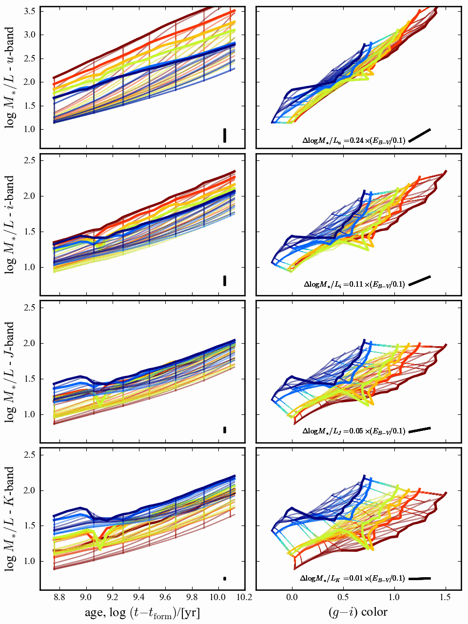
Figure 10: Variations in $M_{*}/L$ as a function of age and colour for models in our SPL.— This Figure is discussed at length in §5.1 and §5.2. Each panel of this Figure shows a projection of our SP model grid. Individual models are colour-coded by their metallicity. The lines connect models that differ in only one of age, $e$-folding time, or metallicity. We only show zero-dust models; the dust vector is given in the lower-right-hand corner of each panel. From top to bottom, the different rows show the spread of $M_{*}/L$s in the $u$-, $i-$, $J$ and $K$-bands within the models; these values are plotted as a function of SP age (left panels), and restframe $(g-i)$ colour (right panels). The results shown in this panel imply that $u$-, $i$-, $J$-, or $K$-band fluxes on their own can be used to infer stellar masses to within a factor of 22, 5.5, 4.0, and 4.5, respectively. That is, on its own, $L_{i}$ is almost as good an indicator of $M_{*}$ as $L_{J}$ or $L_{K}$. At the same time, the variation in $M_{*}/L_{i}$ at fixed $(g-i)$ is considerably smaller: $M_{*}/L_{i}$ can in principle be predicted to within a factor of 2 using $(g-i)$ colour alone.

5.2.1 The effects of dust

In what we have said so far in this Section, we have completely ignored dust. This may have seemed like a very important oversight, so let us now address this issue. The dust vector in $(g-i)$–$M_{*}/L_{i}$ space is ($\Delta(g-i),~{}\Delta(\log M_{*}/L_{i})$) = (0.19, 0.11) $\times\mathrm{E}_{B\text{-}V}/0.1$. Compare this to the empirical $(g-i)$–$M_{*}/L_{i}$ relation for GAMA galaxies, which, as we show in §5.3 below, has a slope of 0.73. Because these two vectors are roughly aligned, the first order effect of dust obscuration is merely to shift galaxies along the $(g-i)$–$M_{*}/L_{i}$ relation (see also Bell & de Jong, 2001; Nicol et al., 2010). This means that the accuracy of $(g-i)$-derived estimates of $M_{*}/L_{i}$ are not sensitive to a galaxy’s precise dust content. Said another way, although there may be large uncertainties in $\mathrm{E}_{B\text{-}V}$, this does not necessarily imply that there will also be large uncertainties in $M_{*}/L_{i}$.

To see this clearly, imagine that we were only to use zero-dust models in our SPL, and take the example of a galaxy that in reality has $\mathrm{E}_{B\text{-}V}=0.1$ mag. In comparison to the zero-dust SPL model with the same $t$, $\tau$, and $Z$, this dusty galaxy’s $(g-i)$ colour becomes 0.19 mag redder, and its absolute luminosity drops by 0.11 dex; the effective $M_{*}/L_{i}$ is thus increased by the same amount. (Recall that $L_{i}$ denotes the effective absolute luminosity without correction for internal dust obscuration, rather than the intrinsic luminosity produced by all stars.) Now, using the slope of the $(g-i)$–$M_{*}/L_{i}$ relation, the inferred value of $M_{*}/L_{i}$ for the $\mathrm{E}_{B\text{-}V}=0.1$ mag galaxy will be $0.70\times 0.19=0.13$ dex higher than it would be for the same galaxy with no dust. That is, in this simple thought experiment, the error in the value of the effective $M_{*}/L_{i}$ implied by $(g-i)$ would be $0.02\times(\mathrm{E}_{B\text{-}V}/0.1)$ dex, even though we would be using completely the wrong kind of SPS model to ‘fit’ the observed galaxy.

Note that this argument holds only to the extent that dust can be accurately modelled using a single dust vector; i.e.a single screen approximation. Using the Fischera & Dopita (2005) attenuation curve, which is a single screen approximation to a fractal dust distribution, does not produce a large change in the derived values of $M_{*}/L$. Using the model of Tuffs et al. (2004) and Popescu et al. (2000), Driver et al. (2007) show how variations in both viewing angle and bulge–to–disk ratio can produce a spread in the color–$M_{*}/L$ dust vectors. These results suggest that in some cases, dust geometry may have a significant effect on the colour-inferred value of $M_{*}/L$, at the level of $\Delta M_{*}/L_{V}\sim 0.1\mathrm{E}_{B\text{-}V}$. One avenue for further investigation of the effects of dust geometry is through detailed radiative transfer modelling for galaxies whose geometries can be accurately constrained. While this is clearly impractical for large galaxy samples, an alternative would be to construct spatially resolved mass maps (see, e.g. Conti et al., 2003; Lanyon-Foster et al., 2007; Welikala et al., 2008; Zibetti et al., 2009), using a single-screen approximation for each pixel individually.

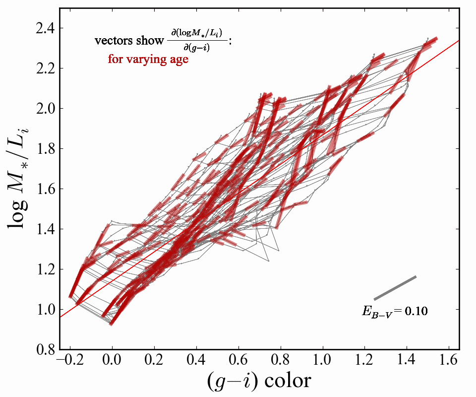
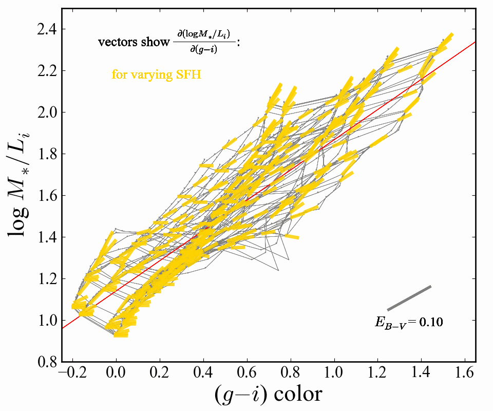
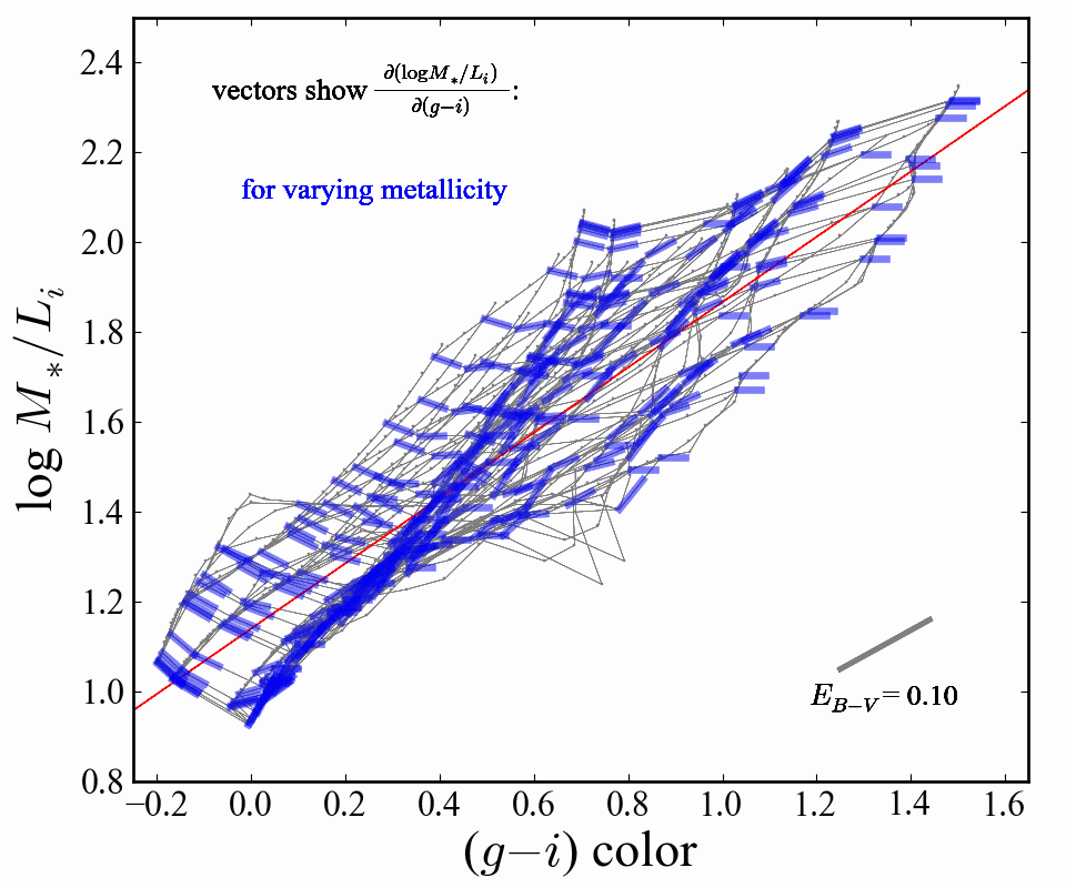
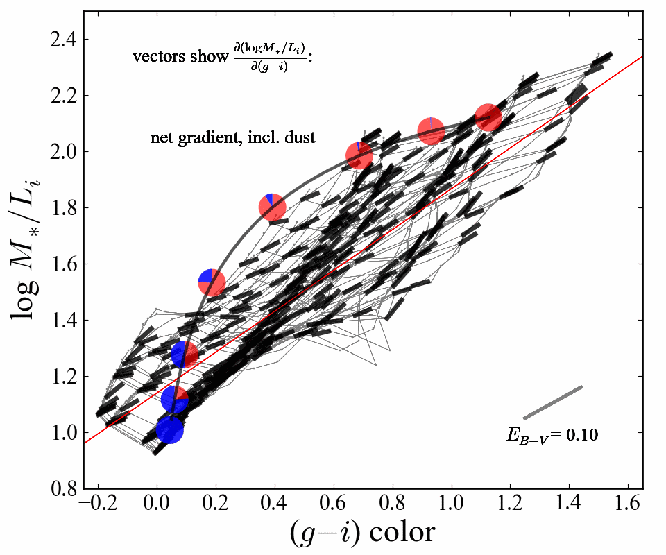
Figure 11: The generic relation between restframe $(g-i)$ colour and $M_{*}/L_{i}$ for the models in our SPL.— The first three panels of this Figure show the movement of the models in our SPL in the $(g-i)$–$M_{*}/L_{i}$ plane with variations age, SFH, and metallicity, respectively. In each of these panels, the vectors show the age, SFH, or metallicity analogues of the dust vector for $\Delta(g-i)=0.05$; that is, the change in $M_{*}/L_{i}$ that is associated with a change in $t$, $\tau$, or $Z$ such that the restframe $(g-i)$ colour changes by 0.05 mag. In the fourth panel, the black vectors show the net variation in $\Delta M_{*}/L_{i}$ with a 0.05 mag change in $(g-i)$, obtained by marginalising over the $t$, $\tau$, and $Z$ priors. The fact that each of these vectors—both individually and en masse—are roughly aligned with one another means that variations in any of these parameters largely preserves both the slope of and scatter in the relation between $(g-i)$ and $M_{*}/L_{i}$ (see §5.2). Further, in the final panel, we provide a qualitative illustration of how multi-component SPs affect the $(g-i)$–$M_{*}/L_{i}$ relation by combining an old and passive SP with a young, star forming one. These are shown as the large circles connected by the smooth black curve. The relative young:old mass ratio is indicated by the relative area of the blue and red regions within each circle for young mass fractions of approximately (right to left) 0, 1, 3, 9, 24, 50, 76, and 100 %. Even for this rather extreme example of multi-component stellar populations, it remains true that $(g-i)$ colour can, in principle, be used to estimate $M_{*}/L_{i}$ to within a factor of $\sim 2$ ($0.3$ dex).

5.2.2 Dependence on $t$, $\tau$, and $Z$

Just as $(g-i)$ can be used to estimate $M_{*}/L_{i}$ without being strongly sensitive to dust, variations in each of age, SFH, and metallicity do not have a large impact on $(g-i)$-inferred estimates of $M_{*}/L_{i}$. This is demonstrated in Figure 11, in which we use our SPL models to show how variations in any one of $t$, $\tau$, or $Z$ shift galaxies in the $(g-i)$–$M_{*}/L_{i}$ plane. We do this as follows: for an individual model, we ask how great a change in any one of $t$, $\tau$, or $Z$ (while holding the other two parameters fixed) is required to change $(g-i)$ by 0.05 mag; we then look at the corresponding change in $M_{*}/L_{i}$ that comes with this variation. In other words, we are looking at how uncertainties in each of $t$, $\tau$, and $Z$ affect the accuracy of $(g-i)$–inferred estimates of $M_{*}/L_{i}$. These are shown as the red, yellow, and blue vectors, respectively.

Focussing on each set of vectors individually, it can be seen that for the bulk of the models, the effect of independent variations in any of $t$, $\tau$, or $Z$ is to move the model point more or less parallel to the main cloud. Note, too, that closer to the centre of the main cloud, the three separate vectors tend to come into closer alignment.

To first order, then, variations in any one of these quantities simply shift galaxies along the main $(g-i)$–$M_{*}/L_{i}$ relation. By the same argument presented above in regard to dust, this implies that $(g-i)$ can be used to infer $M_{*}/L_{i}$ to high accuracy, even if the ‘best fit’ model of the same $(g-i)$ colour has completely the wrong values of $t$, $\tau$, or $Z$. Figure 11 thus shows that, uncertainties in any of $t$, $\tau$, and $Z$ do not produce large errors in the value of $M_{*}/L_{i}$ inferred from the $(g-i)$ colour.

5.2.3 The net covariance between $M_{*}/L_{i}$ and $(g-i)$

Considering the combined effect of variations in all three of $t$, $\tau$, and $Z$, the robustness of $(g-i)$–derived estimates of $M_{*}/L_{i}$ is even greater. The black vectors in this plot show the net variation in $M_{*}/L_{i}$ allowing for the uncertainties in all of $t$, $\tau$, and $Z$ that come with an observational uncertainty of $\Delta(g-i)=0.05$. Notice how closely aligned these vectors are with the empirical $(g-i)$–$M_{*}/L_{i}$ relation for real galaxies.

This shows that while there may well be a relatively large range of models with different values of $t$, $\tau$, and/or $Z$ that are consistent with the observed value of $(g-i)$ for any given galaxy, because all of these models will follow more or less the same relation between $(g-i)$ and $M_{*}/L_{i}$, the spread of $M_{*}/L_{i}$s among these models will still be relatively low. That is, through a coincidence of dust and SP evolution physics, the dust–age–metallicity degeneracy actually helps in the estimate of $M_{*}/L_{i}$ (see also, e.g. Bell & de Jong, 2001; Nicol et al., 2010). Furthermore, as a corollary to this statement, because the estimated value of $M_{*}/L_{i}$ does not depend strongly on the accuracy of the inferred values of $t$, $\tau$, $Z$, or $\mathrm{E}_{B\text{-}V}$, it is not necessary to model these aspects of the SPL models exactly.

5.2.4 Multicomponent stellar populations

The last commonly-cited bugbear of stellar mass estimation is the effect of ‘secondary’ populations in general, and of bursts in particular, on the inferred value of $M_{*}/L$. To explore this issue, consider the case of a combination of two SPs with ($t$, $\tau$, $Z$) = (10 Gyr, 0.5 Gyr, $Z$_⊙) and (0.5 Gyr, 30 Myr, $Z$_⊙); i.e., an old and passive SP and a very young and star forming SP. These two individual SPs are highlighted in the fourth panel of Figure 11. Now let us combine these two SPs in varying amounts. The track connecting these two points show where the combined SP would lie in the $M_{*}/L_{i}$–$(g-i)$ plane. The large points highlight the cases where the mass of the burst component is $10^{-2}$, $10^{-1.5}$, …, $10^{0.5}$ times the mass of the old component.

We again see that the $M_{*}/L_{i}$–$(g-i)$ relation is largely preserved. In particular, the effect of small bursts ($f_{\mathrm{young}}\lesssim 0.05$) on the $M_{*}/L_{i}$–$(g-i)$ colour relation is very slight. At least for the specific case that we have chosen to illustrate, we see that if a very old galaxy were to experience a modest burst ($0.05\lesssim f_{\mathrm{young}}\lesssim 25$ %), then this will shift the galaxy along the edge of the main cloud. The greatest concern is a largely star-forming galaxy with a sizeable underlying population of very old stars ($0.25\lesssim f_{\mathrm{old}}>\lesssim 0.75$). In this case, $M_{*}/L_{i}$ can shift by up to 0.5 dex with only a small change in colour; $\Delta(g-i)\lesssim 0.2$.

It is thus clear from this panel that secondary stellar populations in general, and those with $0.25\lesssim f_{\mathrm{young}}\lesssim 0.75$ in particular, are better able to shift galaxies away from the main $M_{*}/L_{i}$–$(g-i)$ relation than are variations in any or all of $t$, $\tau$, $Z$, or $\mathrm{E}_{B\text{-}V}$ within one of our smooth and exponential CSPs. That said, we stress this specific example represents something of an extreme case: the two separate SPs we have chosen are at opposite ends of the SP values that we find for real galaxies, and the problem is only significant where the two populations are comparable in mass. Furthermore, even for this extreme example, note that the combined SP still lies within the main cloud of SPs within our SPL. The claim that $M_{*}/L_{i}$ can be estimated to within a factor of $\lesssim 2$ based on the $(g-i)$ colour alone is true even for galaxies with relatively complex SFHs.

5.3 The empirical relation between $\mathbf{(g-i)}$ and $\mathbf{M_{*}/L_{i}}$

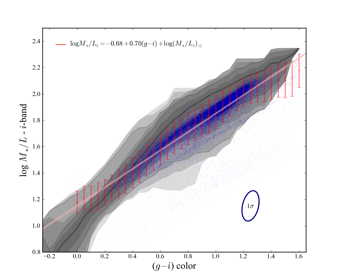
Figure 12: The empirical relation between restframe $(g-i)$ colour and $M_{*}/L_{i}$.— The points show the inferred values of $(g-i)$ and $M_{*}/L_{i}$ for galaxies in the GAMA catalogue. The red points show the median value of $M_{*}/L_{i}$ in narrow bins of $(g-i)$; the error bars on these points reflect the median $\pm 1\sigma$ upper and lower limits on $M_{*}/L_{i}$ in each bin. These error bars thus reflect the combination of the (small) intrinsic scatter in the $(g-i)$–$M_{*}/L_{i}$ relation and the (larger) observational uncertainties in $M_{*}/L_{i}$ at fixed $(g-i)$. The solid red line shows the best fit to the empirical relation between $(g-i)$ and $M_{*}/L_{i}$, with the form as given at top left. In fitting this relation, we have fully accounted for the covariant errors in $(g-i)$ and $M_{*}/L_{i}$; the median error ellipse is shown at bottom right. For comparison, the underlaid greyscale contours show the prior-weighted distribution of $M_{*}/L_{i}$s for the models in our SPL, computed in narrow bins of $(g-i)$. The heavy central line shows the prior-weighted median, and the contours are spaced at the equivalent of the $\pm 0.5$, 1.0, … 3.0 $\sigma$ percentiles of the prior-weighted distribution. The observed relation for real galaxies is both more nearly linear and tighter than might be expected from the models alone. This implies both that the full $ugriz$ SED contains additional information concerning a galaxy’s stellar population not embodied in the $(g-i)$ colour alone, and that the precise form of and scatter around the $(g-i)$–$M_{*}/L_{i}$ relation is a product of galaxies’ formation and evolutionary histories. In this sense, we have calibrated the ($g-i$)–$M_{*}/L_{i}$ relation such that, modulo uncertainties in the stellar population models used to derive these values, the $(g-i)$ colour can be used to predict $M_{*}/L_{i}$ to a $1\sigma$ accuracy of $\approx 0.10$ dex.

So far in this Section, our discussion has been restricted to the range of $M_{*}/L$s and colours spanned by the models in our SPL, and has thus focussed on the theoretical relation between $(g-i)$ and $M_{*}/L_{i}$. In this sense, our conversation has been completely generic—at least insofar as the SP models we have used provide an accurate description of the stellar content of real galaxies.

Let us now turn to Figure 12, and consider how well $(g-i)$ can be used to estimate $M_{*}/L_{i}$ in practice. In this Figure, the grey-scale contours show the prior-weighted distribution on $M_{*}/L_{i}$ for the models, again in bins of $(g-i)$, as the grey-scale contours: the darkest line shows the median prior-weighted value; the greyscale shows the equivalent of the $\pm 0.5$, 1.0, …, 3.0 $\sigma$ percentiles. This Figure also shows the empirical relation between $(g-i)$ and $M_{*}/L_{i}$ that we infer for real GAMA galaxies, based on our $ugriz$ SPS fits. The data themselves are shown as the blue points.

Consider for a moment what would happen if we were to have only (restframe) $g$- and $i$-band photometry for a real galaxy. The inferred value of $M_{*}/L_{i}$ would just be the mean value of all models in our SPL with a similar colour (weighted both by the consistency between the observed and model photometry, and the prior probability of that model). Further, for a given $(g-i)$, the inferred uncertainty in $M_{*}/L_{i}$ would simply reflect the prior-weighted range of values spanned by models of the same colour. That is, we would expect to ‘recover’ the prior-weighted distribution shown as the grey contours in Figure 12.

This is not what we see for the real galaxies: there are clear differences between the form of and scatter around the relations between $(g-i)$ and $M_{*}/L_{i}$ for the models on the one hand, and for the data on the other. Particularly for intermediate colours, the median value of $M_{*}/L_{i}$ is considerably lower than the probability-weighted mean of the models. This demonstrates that the $u$-, $r-$, and $z$-band data do provide additional information concerning $M_{*}/L_{i}$ that cannot be gleaned from $(g-i)$ alone.

Further, the effect of this additional information is to significantly reduce the observed scatter in the relation between $(g-i)$ and $M_{*}/L_{i}$. The red points in Figure 12 show the median values of $M_{*}/L_{i}$ for GAMA galaxies in narrow bins of $(g-i)$. The error bars on these points show the mean values of the formal 1$\sigma$ upper and lower limit on $M_{*}/L_{i}$ in each bin; these error bars thus show the intrinsic, astrophysical scatter in the relation convolved with the formal, observational uncertainties. Even considering the formal uncertainties for individual galaxies, the scatter around the mean colour–$M_{*}/L_{i}$ relation is considerably lower than what would expected from the models alone: quantitatively, the scatter in $M_{*}/L_{i}$ is constrained to being $\lesssim 0.1$ dex for all values of $(g-i)$. This shows that, the apparent tightness of the relation between $(g-i)$ and $M_{*}/L_{i}$ is not a mere consequence of the central limit theorem.

In other words, the precise form of the empirical relation between $(g-i)$ and $M_{*}/L_{i}$ encodes information about the distributions of SPs among real galaxies. Both the linearity and tightness of the observed relation are therefore fortuitous coincidences of the physics of galaxy formation and evolution.

Fitting the empirical relation for GAMA galaxies, we find:

$$\log M_{*}/L_{i}=-0.68+0.70(g-i)~{}.$$ (7)

(To convert $L_{i}$ from our preferred AB-centric units to Solar units, note that the absolute AB magnitude of the sun in the $i$-band is $M_{i,\odot}=4.58$.) This fit is shown in Figure 12 as the solid red line. In the fitting, we have fully accounted for the covariant errors in the derived values of $(g-i)$ and $M_{*}/L_{i}$; the mean error ellipse is shown in the lower-right corner of this panel. Rearranging Equation 7 to put all observables to one side, we have in effect calibrated the empirical relation between $(g-i)$ colour, $i$-band luminosity, and stellar mass as:

$$\log M_{*}/[M_{\odot}]=-0.68+0.70(g-i)-0.4M_{i}~{},$$ (8)

where $M_{i}$ is the absolute magnitude in the restframe $i$-band, expressed in the AB system. This relation can be used to estimate $M_{*}/L_{i}$ to a 1$\sigma$ accuracy of $\sim$ 0.10 dex using (restframe) $g$- and $i$-band photometry alone.

5.4 Comparison with other recent works

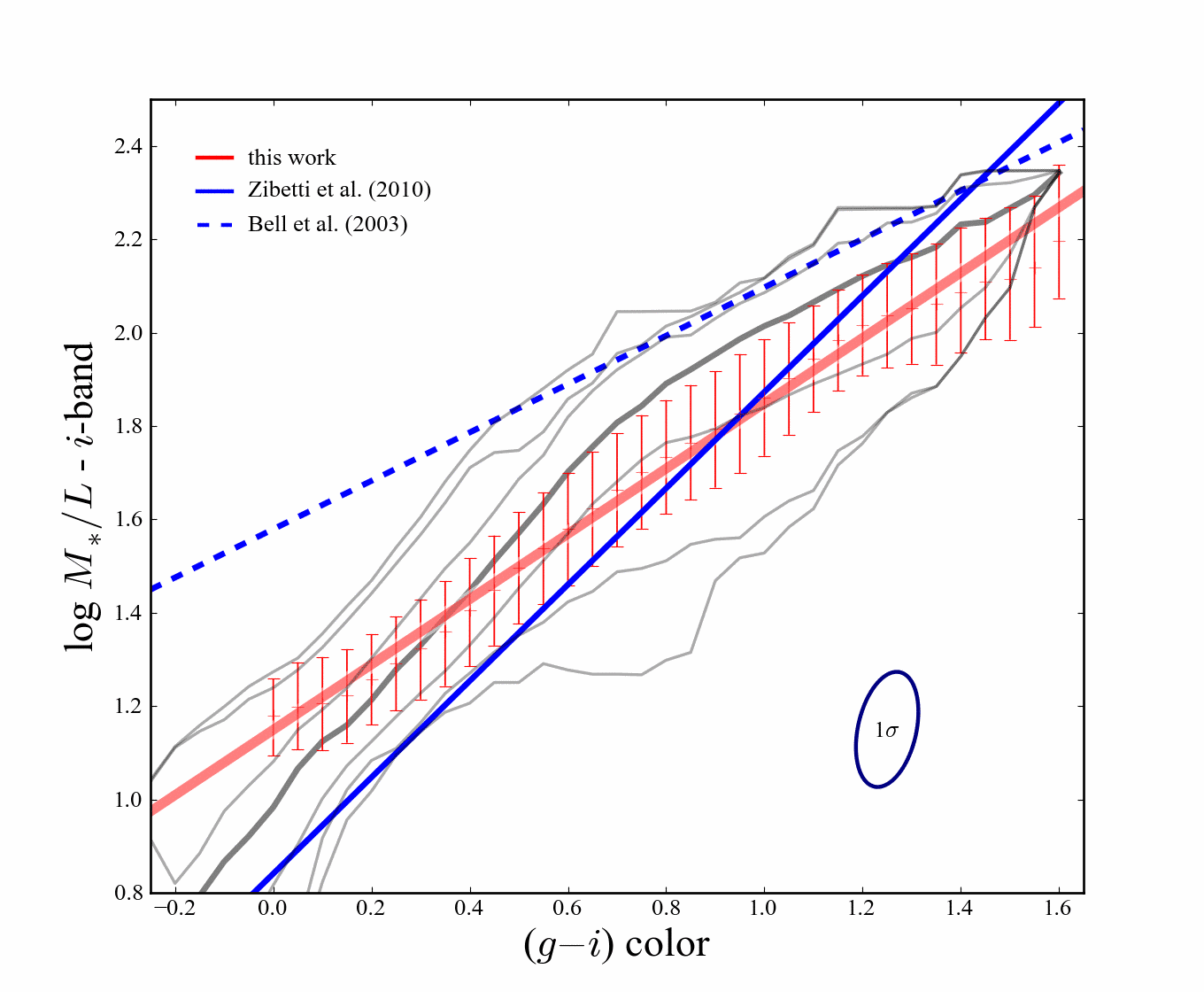
Figure 13: Comparison between our empirical $M_{*}/L_{i}$–$(g-i)$ relation and other recent works.— The dashed and solid blue lines in this Figure shows the relations between $M_{*}/L_{i}$ and $(g-i)$ presented by Bell et al. (2003) and Zibetti et al. (2009), respectively; all other symbols are as in Figure 12. The Bell et al. (2003) relation has been derived for galaxies from the SDSS EDR, and should thus be compared to our empirical relation. Note, however, that the Bell et al. (2003) relation should be understood to include evolution corrections. The Zibetti et al. (2009) relation has been obtained by marginalising over the models in their SPL in bins of $(g-i)$. This relation thus cannot be considered to be ‘empirical’, and should be compared to the prior-weighted median for our SPL, shown as the heavier grey line. The significant systematic differences between these relations underscore the importance of ensuring that any cross-survey comparisons are based on a comparable mass scale.

In Figure 13, we compare our empirically calibrated $M_{*}/L_{i}$–$(g-i)$ relation to two other recent works. From the outset, let us stress that these relations are not directly comparable, in the sense that they have been derived in very different ways, and therefore should be interpreted as having rather different meanings.

First, the dashed blue line shows the relation given by Bell et al. (2003), which has been derived from least-squares SED fitting to $ugriz$ SEDs for galaxies from the SDSS Early Data Release (EDR Stoughton et al., 2002) coupled with $K$-band photometry from 2MASS (Cutri et al., 2003; Skrutskie et al., 2006), and using Pegase (Le Borgne & Rocca-Volmerange, 2002) SSP models as the basis of the SPL. We have scaled the Bell et al. (2003) relation down by 0.093 dex to account for their use of a ‘diet Salpeter’ rather than Chabrier (2003) IMF. Most importantly, Bell et al. (2003) explicitly attempt to account for evolution between the epoch of observation and the present day by running forward the implied SFH to $z=0$. With that caveat, the Bell et al. (2003) relation is derived from fits to the observed relation between $M_{*}/L$ and colour for real galaxies in a similar way as in this work, and so can be compared to our relation, shown in Figure 13 as the solid red line.

Second, the solid blue line shows the relation derived by Zibetti et al. (2009), which is based on a Monte Carlo realised SPL modelled after Kauffmann et al. (2003a) (i.e., including secondary SF bursts), with a sophisticated treatment of dust extinction using the formalism of Charlot & Fall (2000). The relation shown has been derived by marginalising over all SPL models in bins of $(g-i)$. The Zibetti et al. (2009) relation should therefore be compared to the heavier gray line in Figure 13, which shows the prior-weighted median value of $M_{*}/L_{i}$, computed in bins of $(g-i)$, for our SPL. That said, there is still one important caveat: Zibetti et al. (2009) have marginalised over their dust priors, whereas the gray line in Figure 13 is based only on the zero-dust models in our SPL. Note that the precise form of the Zibetti et al. (2009) line is determined almost entirely by their assumed priors (i.e., the relative weighting given to the different models in their SPL); no observational data has been used to derive this relation.

The reader may be forgiven for being startled by the apparently poor agreement between these relations in the first instance, and then equally by the subtleties in their meanings. The point to take from this comparison is simply that there are important systematic differences between each of these mass determinations. (Although, again, we stress that we have shown our $M_{*}/L_{i}$ estimates to be in excellent agreement with the well-tested and widely used SDSS values.) It is clear from Figure 13 that comparing results based on different mass determination methods would not be fair, or at best, would be misleading. The utility of these relations is therefore primarily that they provide a means for simply and transparently reproducing the results of more sophisticated calculations, ‘warts and all’; i.e., including any and all systematics. The derived relation between $(g-i)$ and $M_{*}/L_{i}$ thus provides a solid basis for comparison between results from GAMA (and, by extension, SDSS), and from other survey projects.

6 Discussion—Where to from here?

In this penultimate Section, we look at how our SP parameter estimates might be improved for future GAMA catalogues. First, in §6.1, we look at what might be gained by successfully integrating NIR data into our SPS calculations. Then, in light of our present difficulties in incorporating the available NIR data, in §6.2, we explore potential avenues for improving on the present SP parameter estimates. In particular, we argue that any future improvements in our SPS calculations will require a new conceptual framework.

6.1 The value of NIR data

Let us now consider what additional information may be provided by the inclusion of NIR data, or, conversely, what we have sacrificed by excluding the available NIR data for the present catalogue of stellar masses and SP parameters. Our discussion of this question is based on Figure 14. As in Figure 10, these panels show the variation in $M_{*}/L$ at different wavelengths for our SPL. The lefthand panels show $M_{*}/L$ as a function of $(g-i)$ colour; the righthand panels show the same as a function of $(i-K)$ colour. Using this Figure, then, we can compare the information encoded in optical–minus–optical and optical–minus–NIR colours.

Figure 14 shows that most of the additional information encoded within optical–to–NIR colours is concerning metallicity: the fact that each of the single-metallicity surfaces are well separated in the righthand panels shows that the different metallicity models can be easily distinguished by their $(i-K)$ colours. While the single-age metallicity surfaces are well-separated, however, the fact that each of these surfaces spans a narrower range of $(i-K)$ colours than $(g-i)$ colours shows that both $t$ and $\tau$ are better constrained by $(g-i)$. That is, the inclusion of NIR data will not necessarily lead to tighter constraints on galaxies’ individual SFHs. Further, by the same argument that we have used in §5.1 and §5.2, it is immediately clear from Figure 14 that the $(i-K)$ colour encodes virtually no information directly pertaining to $M_{*}/L$: the range of $M_{*}/L$ within our SPL is nearly constant as a function of $(i-K)$. To be sure, optical–to–NIR SED shape is a powerful means of breaking degeneracies associated with metallicity, but this has very little bearing on the inferred value of $M_{*}/L_{i}$.

In this way, Figure 14 offers a means of understanding the results of the numerical experiments presented in Appendix A. In this Appendix, we find that the principal gain that comes with the inclusion of the NIR is in our ability to recover the known values of $Z$ for the mock galaxies. Although the inclusion of NIR data has little to no effect on our ability to recover $t$ or $\tau$ individually, our ability to recover $\left<t_{*}\right>$ is improved (from $\sim 80$ % to $\sim 55$ %) with the inclusion of the NIR. That is, while NIR data do help to break the degeneracy between metallicity and luminosity-weighted mean stellar age, it does not help to constrain galaxies’ precise SFHs. We also find that including the NIR data has little effect on our ability to recover the known values of $M_{*}/L$ for synthetic galaxies: we are able to recover the known values of $M_{*}/L$ to within $\approx 0.05$ and $\approx 0.06$ dex with and without the inclusion of NIR data, respectively.

We therefore conclude that the robustness and reliability of our stellar mass estimates will not necessarily be improved simply by folding the NIR data into the SPS calculations—or, said another way, our decision to exclude the NIR data for the current catalogue does not necessarily have a large adverse effect on the quality of our stellar mass estimates.

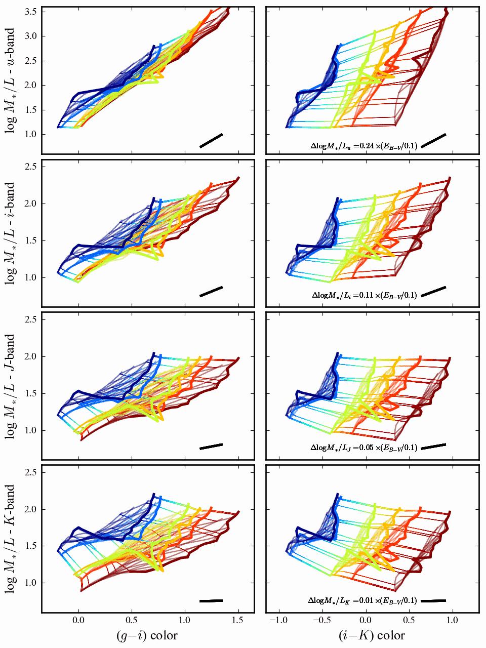
Figure 14: Variations in $M_{*}/L$ as a function of restframe $(g-i)$ and $(i-K)$ colour for models in our SPL.— All symbols and their meanings are as in the directly comparable Figure 10. In contrast to $(g-i)$, optical–minus–NIR colours contain virtually no information directly pertaining to $M/L$, or to age. Instead, the optical–to–NIR colour is sensitive primarily to variations in dust and metallicity. While the inclusion of NIR data into the SPS fitting calculation may in principle lead to tighter constraints on $t$, $\tau$, $Z$, and $\mathrm{E}_{B\text{-}V}$, it will have little to no impact on the accuracy of our $M_{*}/L$ estimates.

6.2 Building a better synthetic stellar population library

In §4.4, we have suggested that our problems in satisfactorily incorporating the available NIR data into the SPS calculation may reflect that our present SPL is inadequate to the task of describing galaxies’ full optical–to–NIR SED shapes. In this Section, with an eye towards the availability of the much deeper VST-KIDS and VISTA-VIKING optical and NIR imaging in the near future, we discuss possible avenues for deriving improved SP parameter constraints. In particular, we are interested in the first instance in what kinds of expansions of our SPL are likely to have the greatest impact on our SPS calculation; secondarily to this, we want to know whether and what modifications to our SPS algorithm will be required to fully exploit these high quality data.

Our discussion is based on Figure 15, in which we show colour-colour diagrams for two heavily populated redshift intervals in the GAMA sample. The coloured lines in Figure 15 show the evolutionary tracks for models in our SPL with different values of $\tau$ and $Z$. Each track is colour-coded according to its metallicity. For clarity, we only show the models with zero dust; the $\mathrm{E}_{B\text{-}V}=0.1$ dust vector is shown at the bottom right of each panel. These tracks should be compared to the actual observations, which are shown as the black points. Based on this Figure, let us now consider how our ability to fit the optical–to–NIR SEDs of real galaxies might change with an expanded SPL template set.

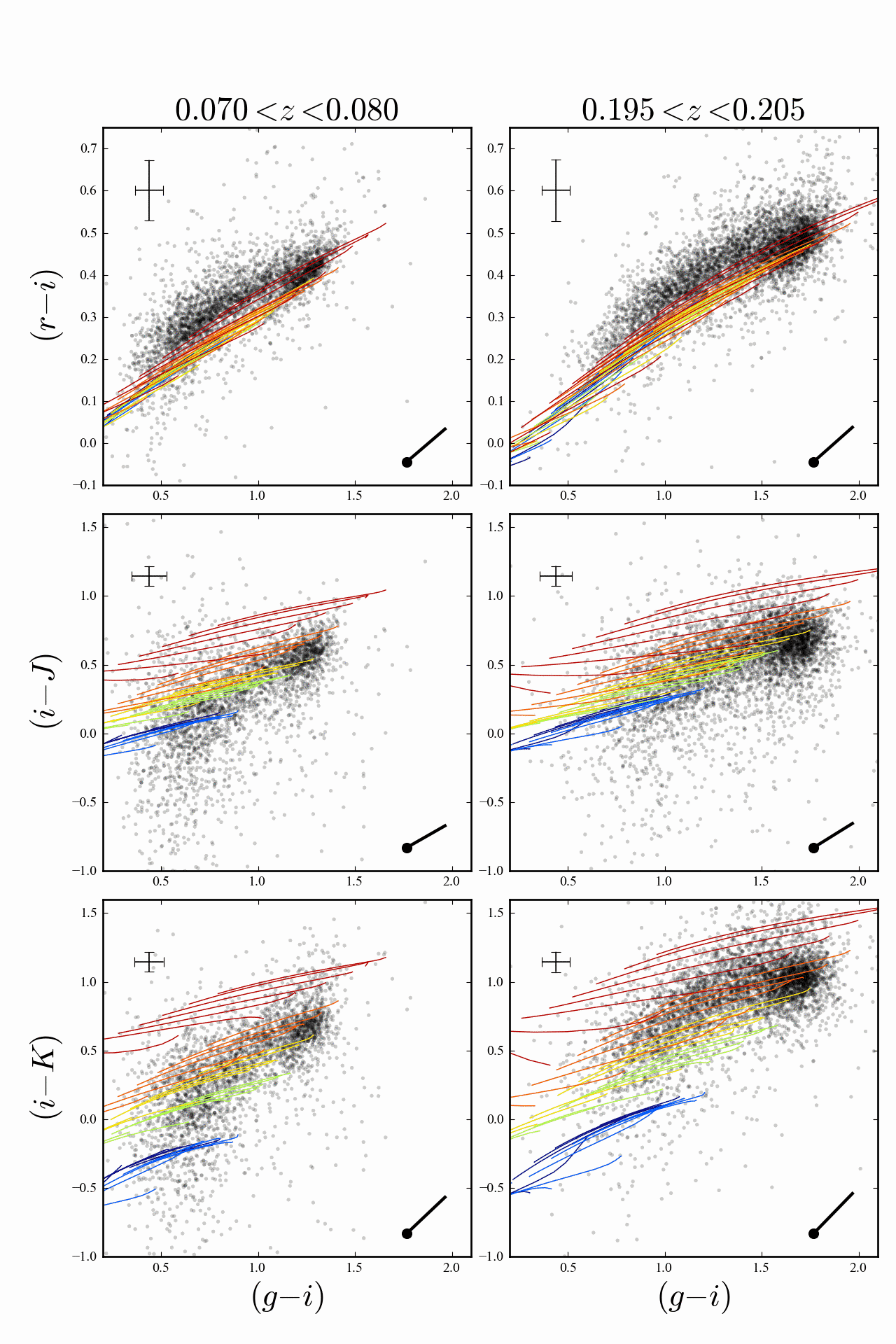
Figure 15: Comparing the model and observed optical and NIR colours for galaxies in two narrow redshift intervals.— Each panel of this Figure shows a (observers’ frame) colour-colour diagram for these two redshift intervals: from top to bottom, we plot $(r-i)$, $(i-J)$, and $(i-K)$ against $(g-i)$. The grey points show the observed colours of GAMA galaxies. We have deliberated selected two well-populated spikes in the GAMA redshift distribution. The coloured tracks show models from our SPL, colour-coded by their metallicity. The $\mathrm{E}_{B\text{-}V}=0.1$ dust obscuration vector is shown in the lower right corner of each panel. The point to be made from this Figure is that the single metallicity stellar populations in our library only sparsely cover the observed optical–NIR colour–colour space of real galaxies. A finer metallicity grid in the stellar evolution models is required for adequate synthetic stellar population modelling including NIR data.

6.2.1 Expanding the metallicity grid

The upper panels of Figure 15 show $(g-i)$ versus $(r-i)$. Note that in the optical, the different uniform metallicity models in our SPL almost completely overlap. But as you go further towards the NIR (lower panels), the distance between the different metallicity tracks steadily grows. Looking at the bottom panels, it is clear that the relatively coarse grid of $Z$ values used for our present SPL only sparsely samples the $giK$ color space of real galaxies. Particularly for the gap between $\log Z=-3.4$ and $-2.4$, the distance between the distinct metallicity tracks in $(i-K)$ becomes comparable to the imposed error floor of 0.05 mag (see §3.2). This explains the origin of the most striking feature of Figure 9: the rather strong quantisation in $Z$. Galaxies with colours that lie between the distinct metallicity tracks can only be fit by adopting the too-blue, lower metallicity model, with the addition of some dust to compensate.

The implication, then, is that a finer grid of metallicities is required when working with NIR data than when working with optical data alone. (This is a direct corollary to the fact that optical–minus–NIR colours are sensitive to metatllicity in a way that optical colours are not.) The problem here is twofold. The first problem is a mundane, practical one: the size of our current SPL is already about as big as we can deal with. With the current architecture of our code, we cannot easily expand the grid in any one dimension without reducing its size in some other dimension to compensate.

The bigger problem is that the BC03 (like the M05 and CB07) SSP models cover only a relatively coarse grid in stellar metallicities. In principle, it is trivial to generate models with arbitrary metallicity by interpolating between the SSP models provided by BC03 , M05 , or whomever. However, at fixed age, the $Z$-dependence of both flux and SP properties is complex. For this reason, we consider it unwise to blindly interpolate between models of different metallicities.

To ensure that our coarse metallicity grid is not responsible for the problems we are seeing with the NIR data, however, we have tried re-fitting the galaxies in our main sample with $z<0.12$ galaxies (i.e., we have reduced the size of our redshift grid by a factor of $\sim 5$) using a finer $Z$ grid for the SPL. This grid, which we have generating by interpolating between the different metallicity SSP models at fixed age and wavelength, spans the same range as the native BC03 SSP grid in 24 logarithmically spaced steps.

Using a finer metallicity grid makes no appreciable difference to the quality of the fits to the optical–plus–NIR data. The biggest difference between the two fits is that, with the finer $Z$ grid, the inferred values of $Z$ for galaxies with $-3.5\lesssim\log Z\lesssim-2.5$ are systematically higher by $\approx 0.3$ dex. But even so, compared to the optical–plus–NIR fits using the native BC03 metallicity grid, the change in the inferred value of $M_{*}/L_{i}$ is less than 0.06 dex for 99 % of galaxies; the median change is $<0.01$ dex. We therefore conclude that simply expanding our metallicity grid does not fix our current problems with incorporating the NIR data into the SPS fits, nor does it significantly improve the accuracy of our stellar mass estimates.

In principle, it is easy to accommodate more sophisticated treatments of mixed metallicities by generalising Equation (3.1) so that the SFR is an explicit function of $Z$ as well as $t$. In practice, however, the principal disadvantage to doing so is that we would want to specify or parameterise the relations between $\psi_{*}(t)$, and $Z(t)$, whether explicitly, or in terms of appropriate priors. (Further, this does not address the issue of whether and how one can safely generate SSP models of arbitrary metallicity.) One simple way to accomplish this would be to assume an exponentially-declining gas accretion rate with a characteristic timescale $\tau_{\mathrm{gas}}$, coupled with assumptions about stellar gas recycling back into the ISM (as done by, e.g., Pégase; Le Borgne & Rocca-Volmerange, 2002). Again, the apparent insensitivity of our $M_{*}/L$ estimates argues against this having a large impact on our stellar mass estimates; it may, however, lead to improvements in our estimates of both $Z$ and $\left<t_{*}\right>$.

6.2.2 Allowing for secondary stellar population components

For the present work, we have limited ourselves to considering smooth, exponentially declining SFHs. A number of authors have attempted to incorporate or allow for more complicated SFHs in their SPS calculations. One approach has been to increase the dimensionality of the SPL parameter space by introducing additional SP components as short bursts (e.g. Kauffmann et al., 2003a; Brinchmann et al., 2004; Gallazzi et al., 2005).

We can also use Figure 15 to explore what impact the inclusion of more complicated SFHs in our SPL might have. Consider what happens to any of the models in Figure 15 with the addition of a secondary burst of star formation. If any two of the models shown in Figure 15 are combined in any proportion, the evolutionary track of the resultant SP must necessarily lie between the individual tracks of the two distinct SP components. If you were to combine any two SPs with the same dust and metallicity, but different SFHs, the result will necessarily still lie trapped within the region of colour space spanned by the smooth models. That is, so long as any secondary stellar population has the same dust and metallicity, it will not be easily distinguishable from any of our existing smooth models.

This insight is significant in terms of the results of Gallazzi & Bell (2009). These authors find that SFH-related degeneracies mean that the inclusion of bursty SFHs among the SPL model templates does little to reduce this bias for bursty galaxies. Further, there is the potential that the inclusion of too many bursty SPL models can lead to biases in non-bursting galaxies. In other words, because these scenarios cannot be distinguished on the basis of their SEDs, a bias in $M_{*}/L$ is inevitable, whether that be a small bias for the many ‘smooth SFH’ galaxies, or a large bias for the fewer bursty galaxies. Note, too, that in this picture, the degree of the bias is strongly dependent on the assumed priors.

The implication from the above, then, is that the inclusion of models with mixed metallicities and/or multi-component SFHs will improve our SP parameter estimates only to the extent that they expand the high-dimensional colour space spanned by the full ensemble of SPL models. And then, multi-component SFHs will only expand the SPL colour space if and only if the different components are allowed to have different amounts of dust and/or metals.

In order to meaningfully incorporate dual-component SPs thus requires the addition of at least five parameters to describe the secondary SP: the equivalent of a ‘formation time’; some characteristic timescale for the secondary SFH (i.e., an $e$-folding time, or some equivalent); its mass relative to the primary; and then both its metallicity, and its dust content. With the current architecture of our SPS code, such an expansion of parameter space is completely impractical.

6.2.3 The need for a new conceptual framework

We would therefore appear to have reached the practical limits of complexity that can be covered by discrete grid-search-like fitting algorithms using a static SPL. Independently of the question of NIR data issues, any future expansion of the model parameter space will have to be accompanied by a change in the conceptual framework that underpins our SPS modelling procedure.

Alternative approaches apply standard dimensionality-reducing techniques, developed in the context of data compression, to the problem. One example is the MOPED algorithm (Heavens, Jiminez & Lahov, 2000; Panter, Heavens & Jiminez, 2003), which uses a variant of principal component analysis (PCA) to efficiently perform a 23-component SPS fit to full SDSS spectra, including a generalised 10-bin SFH (see also VESPA; Tojeiro et al., 2008). Another example is kcorrect (Blanton & Roweis, 2007), which uses the technique of non-negative matrix factorisation (NMF). The idea here is to determine the basis set of template spectra that optimally describes the observed SEDs of real galaxies. The NMF basis set is constructed as a combination of SP template spectra; this means that the basis templates constructed using the NMF algorithm can be considered as SPS template spectra with realistic, multi-component, non-parametric SFHs. The principal motivation for and advantage of these approaches is that they can eliminate entirely the need to assume parametric forms for the SFH. In the context of the above discussion, the operational advantage of such approaches can be thought of as shifting from sampling a static and semi-regular grid of parameter values to a dynamic sampling of an expanded but continuous parameter space.

The main point to take from the above discussion is that proper modelling of the optical-to-NIR SED shapes of galaxies is considerably more challenging than modelling just the optical SED. Part of the reason for this is that, for a fixed optical colour, a galaxy’s optical–NIR colour is sensitive to both $Z$ and to $\left<t_{*}\right>$. Said another way it is precisely because a galaxy’s optical–NIR SED can break metallicity-related degeneracies that it becomes necessary to model each of these quantities in more detail—indeed, in more detail than is practical within the present architecture of our code. On the other hand, the relatively strong degeneracies between a galaxy’s SP properties and its optical SED shape means that SPS fitting of optical SEDs can be done using a relatively crude SPL.

7 Summary

The primary purpose of this work has been to present and describe the ‘first generation’ estimates of stellar mass and other ancillary stellar population parameters for galaxies in the GAMA survey. We have deliberately set out to use widely used and accepted techniques to derive these values, partially in order to allow for the fairest comparison between results from GAMA and other high and low redshift galaxy surveys. Our stellar mass estimates are based on the synthetic stellar population models of BC03 , assuming a Chabrier (2003) IMF and a Calzetti et al. (2000) dust law (§3.1). In constructing the stellar population library that forms the backbone of the calculation, we have used the standard assumptions of a single metallicity and a continuous, exponentially-declining star formation history for all stellar populations, with dust modelled as a single, uniform screen (§3.2).

The most significant ‘non-standard’ element of the calculation is that we use a Bayesian approach when determining the fiducial values of all parameters and their associated uncertainties (§3.3). As we show in Figure 5, this decision has an important systematic effect on the parameter estimates: averaged over the full GAMA sample, the most likely (in a Bayesian sense) values of $M_{*}/L_{i}$ are $\sim 0.10$ dex higher than those taken from the single best fit (i.e., maximum likelihood) SP template. While the MPA-JHU mass estimates for SDSS used a Bayesian approach, this is not (yet) generally done in high redshift studies.

Comparisons between GAMA and SDSS

Through comparison between the GAMA- and SDSS-derived values of $M_{*}/L$ and $M_{*}$ (Appendix B), we highlight two important issues with the SDSS model photometry. First, we show that as a measure of total flux, the SDSS model photometry has serious systematics as a function of (true) Sérsic-index (Figure 19). For galaxies best-fit by an exponential model profile, the differential bias between $n\sim 0.5$ and $n\sim 1.5$ is $\gtrsim 0.2$ mag ($\sim 20$ %); for those best-fit by a de Vaucouleurs model profile, the differential bias between $n\sim 2$ and $n\sim 8$ is $\approx 0.7$ mag (a factor of 2). These systematic biases in total luminosity translate directly to biases in total stellar mass: this may be the single largest source of error in the SDSS mass estimates based on model photometry.

Second, if we apply our algorithm to the SDSS model SEDs, we see very large differences between our derived values and those from the MPA-JHU catalogue (Figure 21). These differences are directly tied to strong systematic differences between the SDSS model and GAMA AUTO colours (§B.1.2), such that the net systematic offset in $(u-z)$ is as large as 0.2 mag (Figure 20). We therefore suggest that it may be more appropriate to use petro SEDs when analysing data from the SDSS photometry catalogues.

Despite these differences in the SDSS and GAMA photometry, the fiducial GAMA values of $M_{*}/L$ are in excellent agreement with those found in the latest generation MPA-JHU catalogue for SDSS DR7 (Section B), which have been shown to be well consistent with dynamical mass estimates (Taylor et al., 2010b). (We investigate the consistency between GAMA-derived stellar and dynamical mass estimates in a companion paper.) As we argue in §B.4, the inclusion of a dust prior in the MPA-JHU stellar mass estimation algorithm may have effectively circumvented the potential bias in stellar population parameters based on the SDSS model photometry; using the GAMA AUTO photometry, we find no need for such a prior.

NIR data (currently) does more harm than good

For the present generation of stellar mass estimates, we have elected not to include the available $YJHK$ NIR photometry in the SED-fitting; the stellar population parameters presented here are based on fits to the optical $ugriz$ SEDs only.

As summarised in §4.4, there are three reasons for this decision. First, none of the commonly used stellar population models (BC03, ; M05, ; CB07, ) provide good fits to the full optical–to–NIR SEDs (Figure 7). Second, while the inclusion of the NIR data does have an impact on the derived values—the median value of $M_{*}$ goes down by 0.15 dex when the NIR data are included—the values derived with the NIR are formally inconsistent with those derived from the just the optical data for a large fraction of galaxies. Both of these points suggest inconsistencies between the optical–to–NIR SED shapes of real galaxies and those of the models in our SPL. The third reason is that we find that the ‘random’ differences in inferred SP parameters—particularly $\mathrm{E}_{B\text{-}V}$, $Z$, and $\left<t_{*}\right>$—using different SSP models are larger than than the formal uncertainties once the NIR data are included. That is, our SP parameter estimates become significantly model dependent when, and only when, the NIR data are used.

That said, the systematic differences in the inferred SP parameters based on different SSP models are small: for $M_{*}/L$, the median difference in the value of $M_{*}/L$ using the BC03 and M05 SSP models is just 0.02 dex. We therefore consider it unlikely that the failure of the models to adequately accommodate the NIR data is due to differences between or uncertainties in the stellar evolution models themselves.

This leaves two possibilities: that there may be problems in the NIR data, and/or that the stellar population library that we have used is insufficient to describe the full range of stellar populations that exist in the local universe. These issues will have to be addressed—both through additional data validation and verification and through expansion of our stellar population library to include additional metallicities and possibly more sophisticated star formation histories—in the construction of future generations of the GAMA stellar mass catalogues. We have discussed possible avenues for expanding our SPL in §6.2, and conclude that any future expansion to our SPL parameter space will have to be accompanied by a change in the conceptual framework of our SPS fitting procedure. We would appear to have reached the practical limit of complexity for a simple grid-search-like approach using a static SPL.

Note that future catalogues will make use of considerably deeper VST optical imaging from KIDS and VISTA NIR imaging from the VIKING survey. In this context, it is highly significant that, even with the present photometry, the accuracy of our SP parameter estimates are not currently limited by signal–to–noise, but by systematics. With the exception of the $u$-band, the photometric errors are smaller than the error floor of 0.05 mag that we have imposed for the fits (see §3.2). The extent to which the deeper data will improve on the present SPS fitting results will depend crucially on how well the data can be self-consistency cross-calibrated, including biases due to PSF- and aperture-matching, colour gradients, and background subtraction, as well as the basic photometric calibration. As a corollary to this, it will be incumbent upon us to ensure that the model photometry in any future SPL can be considered accurate to the same level as the real data; $\textit{i.e.},\lesssim 0.05$ mag.

The robustness and reliability of our optical-derived stellar mass estimates

In light of our decision to ignore the presently available NIR data, we have reexamined the commonly-held belief that NIR data are crucial to deriving a robust and reliable estimate of stellar mass (§5). We use generic properties of the stellar population models to demonstrate that on its own, the $i$-band flux is nearly as good a representation of the total stellar population as is the NIR flux (§5.1). More quantitatively, assuming a constant $M_{*}/L_{i}$ or $M_{*}/L_{K}$, it is possible to use $L_{i}$ or $L_{K}$ to estimate $M_{*}$ to within a factor of 5.5 or 4.5, respectively.

Using a similar argument, we show that the variation in $M_{*}/L_{i}$ at fixed $(g-i)$ is $\lesssim 0.5$ dex (Figure 10). The effect of dust is largely to shift galaxies along the $(g-i)$–$M_{*}/L_{i}$ relation. Dust thus does not significantly affect one’s ability to estimate $M_{*}/L_{i}$ using $(g-i)$. Similarly, we show that, for a given model, variations in age, SFH, and metallicity act to largely preserve the relation between $M_{*}/L_{i}$ and $(g-i)$ colour (Figure 11). Further, we show that multi-component stellar populations (e.g., a burst superposed over an old and passive stellar population) fall within the same region of $(g-i)$–$M_{*}/L_{i}$ space as the exponentially-declining star formation histories that comprise our stellar population library. In this way, based on generic properties of stellar evolution models, we show that $(g-i)$ colour can be used to estimate $M_{*}$ to within a factor of $\lesssim 2$, even considering the well known dust–age–metallicity degeneracy, and even for multi-component stellar populations (§5.2).

Finally, we consider the empirical relation between $M_{*}/L_{i}$ and $(g-i)$ for GAMA galaxies. It is significant that the observed relation between $M_{*}/L_{i}$ and $(g-i)$ is both more linear and considerably tighter (at fixed colour, the scatter in $M_{*}/L_{i}$ is $\lesssim 0.1$ dex) than we might expect by simply taking the prior-weighted average of the models in our stellar population library (Figure 12). This implies that the full $ugriz$ SED shape contains additional information not found in the $(g-i)$ colour, and that this information is sufficient to exclude a significant range of the models in our library. The tightness of the $(g-i)$–$M_{*}/L_{i}$ relation is not merely a consequence of the central limit theorem.

In other words, there are two completely separate reasons why $(g-i)$ is an excellent predictor of $M_{*}/L_{i}$, both of which are entirely fortuitous. First, variations in age, SFH, dust, and metallicity—independently and en masse—largely preserve the $(g-i)$–$M_{*}/L_{i}$ relation. This is a coincidence produced by the physics of stellar evolution. Second, the stellar populations of real galaxies produce a $(g-i)$–$M_{*}/L_{i}$ relation that is both tighter and more nearly linear than might be expected from stellar population models alone. This is a coincidence produced by the physics of galaxy formation and evolution.

In this sense, presuming that both our derived values and their associated uncertainties are reasonable, we have effectively ‘calibrated’ the $(g-i)$–$M_{*}/L_{i}$ relation to a precision of $\lesssim 0.1$ dex ($1\sigma$). The derived relation offers a reliable and robust means for observers to derive stellar masses based on minimal information. Similarly, under the (non-trivial) assumption that the relation does not evolve strongly with redshift, it offers a simple and transparent basis for fair comparison between results derived from GAMA and other low- and high-redshift surveys. As an important caveat on the use of this relation, however, any and all systematic errors or uncertainties in the SPL itself—including, e.g., the IMF and errors in the treatment of the optical stellar evolution tracks—are not included in the quoted uncertainty of 0.1 dex. On the other hand, the relation given does offer a solid means for other surveys to compare their stellar mass-centric measures to those from GAMA under the identical assumptions.

Concluding remarks

The stellar mass estimates we have described have been or will be used for a wide variety of recent and ongoing studies by the GAMA collaboration. These include studies of variability in the stellar IMF Gunawardhana et al. (2011), measurement of the $z\approx 0$ mass function (Baldry et al., in prep.), the properties of galaxies at the lowest end of the H$\alpha$ luminosity function (Brough et al., 2011), and studies of galaxy demographics in the field (Taylor et al. in prep.), in groups (Prescott et al. in prep.), and in filaments (Pimbblett et al. in prep.). Further, they provide an important benchmark for any and all future GAMA stellar mass and SP parameter estimates.

In line with the legacy goals of the GAMA survey, these stellar mass estimates are also being made publicly available for use by the wider astronomical community as part of GAMA DR 2 (scheduled for mid-2011). GAMA’s unique combination of depth and survey area have been deliberately chosen to bridge the gap between large-scale local universe surveys like 6dFGS, SDSS and 2dFGRS, and deep surveys of the high redshift universe like VVDS, DEEP-2, and zCOSMOS. Particularly in combination with these other major surveys, the GAMA catalogues are intended to provide a valuable laboratory for studies of galaxy formation and evolution.

Appendix A Numerical Experiments—
SPS fitting of mock galaxy photometry

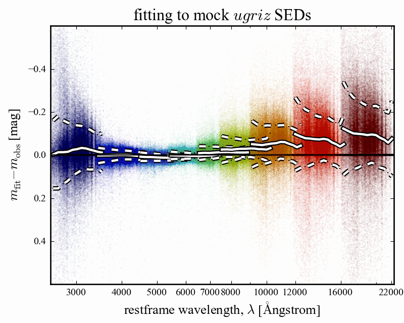
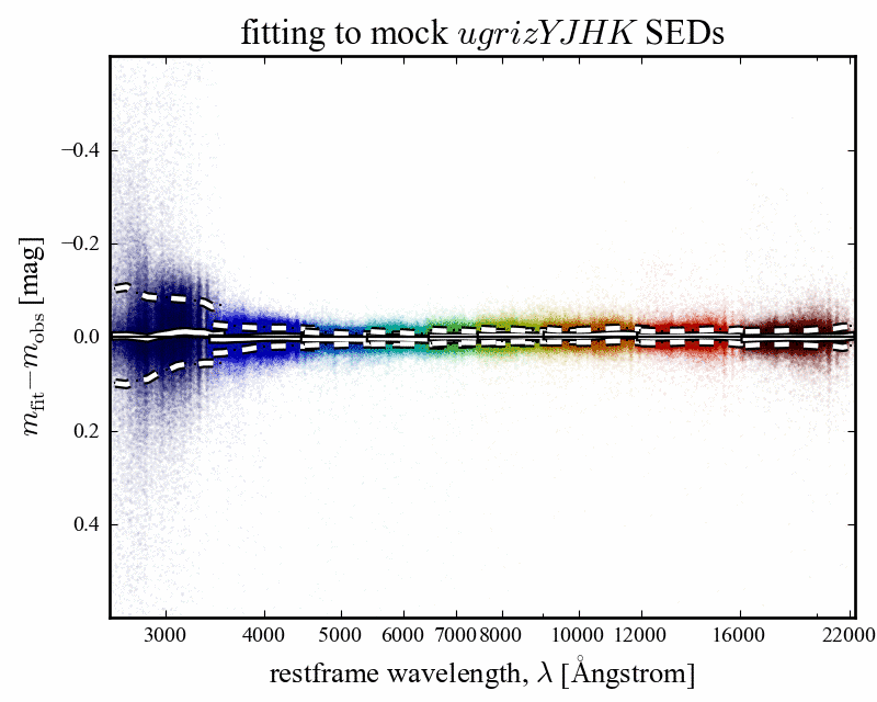
Figure 16: Quality of the SED fits for mock galaxy photometry.— This Figure shows the residuals from the SED fits to the mock galaxy photometry described in Appendix A. The left-hand panel shows the residuals when fitting only the the optical $ugriz$-bands; the right-hand panel shows those for fits to the full $ugrizYJHK$ SEDs. All symbols and their meanings are as in Figure 7, to which these plots should be compared. As argued in §A.1, the fact that the optical–only fits tend to over-predict the ‘true’ NIR fluxes is possible due to the mismatch between our assumed priors and the ‘true’ multi-variate distribution of SP parameters within the mock catalogue. At least qualitatively, the similar residuals seen in Figure 7 for the real galaxies does not then suggest that the fits are necessarily ‘bad’. Further, and in contrast to Figure 7, we are able to reproduce or describe the full optical–to–NIR shapes of the mock galaxies. This strongly suggests that the large residuals seen in Figure 7 are due to problems in the data, short-comings in the SPL models, or both. In any case, the large systematics seen in the right-hand panels of Figure 7 do give reason to treat the results of the optical–to–NIR SED fits with some suspicion.

In this Appendix, we examine our ability to recover the known SP parameters of a set of mock galaxies with a realistic distribution of SP parameters. To this end, we have used the results of our ‘live’ SPS fits to the real GAMA $ugriz$ data to construct a catalogue of mock galaxy photometry. Specifically, for each galaxy, we have take the SPL template SED that most closely matches its ‘most likely’ SP values, added random perturbations commensurate with the actual observational uncertainties for the original galaxy, and then fed that photometry back into the SPS fitting algorithm. Note that the distribution of SP parameters in this mock catalogue is, by construction, the same as what we observe for GAMA galaxies; i.e., it is quite different to our assumed priors.

In §4.1, we have argued that our seeming inability to satisfactorily fit the optical–to–NIR SEDs of GAMA galaxies calls into question the validity of SP parameter estimates inferred from such fits. We have also argued that our inability to predict NIR photometry based on just the optical SEDs—with the implication that the NIR contains additional information not found in the optical—does not imply that the optical cannot be used to reliably infer stellar mass-to-light ratios. In order to provide context for these arguments, we will first spend some time looking at the quality of the photometric fits to the mock photometry in §A.1. We will then go on to look at how accurately and precisely we can recover the known SP parameters of the mock galaxies in §A.2.

A.1 Quality of fits

A.1.1 How well can you fit the optical–to–NIR SEDs?

In the Figure 16, we show the analogue of Figure 7 for this mock galaxy catalogue. Let us look first at the right-hand panel of this Figure, in which we show the difference between the known, input photometry, and the recovered, output photometry, after fitting to the mock $ugrizYJHK$ SEDs. Put simply, the quality of the fits is near perfect. The residuals are at the millimag level for all but the $u$-band; the median residual in the $u$-band is still just 0.02 mag. None of these residuals is significant at the 0.1$\sigma$ level.

A.1.2 How well can you predict NIR photometry based on optical SEDs?

Now consider the left-hand panel of Figure 16, in which we show the residuals when fitting to the mock $ugriz$ SEDs. Our primary interest here is in how well we are able to predict NIR photometry for the mock galaxies using their $ugriz$ SEDs. In comparison to Figure 7, there are three features of this plot that we find striking.

First, it is clear that, as in Figure 7, the NIR photometry predicted from the mock optical SEDs is systematically too bright. Quantitatively, in comparison to Figure 7, the size of the discrepancy is considerably smaller. For the mock galaxies, the residuals are $\lesssim 0.1$ mag; roughly half that seen for real GAMA galaxies. Compared to the photometric errors, the median significance of these offsets is $0.5$, $0.7$, $1.3$, and $1.7\sigma$ in the $YJHK$ bands; again, roughly half that seen in Figure 7.

Second, the residuals for the mock galaxies show a qualitatively different dependence on rest-frame wavelength/redshift than is seen in Figure 7. Whereas for real galaxies, the offsets in each individual band appear to be greatest at the highest and lowest redshifts, for the mock galaxies, the offsets grow rather smoothly for longer and longer wavelengths. That is, for the mock galaxies, our results suggest that one’s ability to predict NIR photometry depends primarily on how far one is willing to extrapolate off the red end of the observed optical SED.

Third, we note that, just as in Figure 7, we do see some residuals in the optical bands. Quantitatively, the median residual in each of the $ugriz$ bands is $-0.02$, $+0.00$, $+0.01$, $+0.00$, and $-0.01$ mag, respectively; in all cases, this is insignificant at the level of $\lesssim 0.2\sigma$. In comparison to those seen in Figure 7, these residuals are again roughly half the size as for real galaxies, but show a qualitatively similar ‘curvature’ with wavelength.

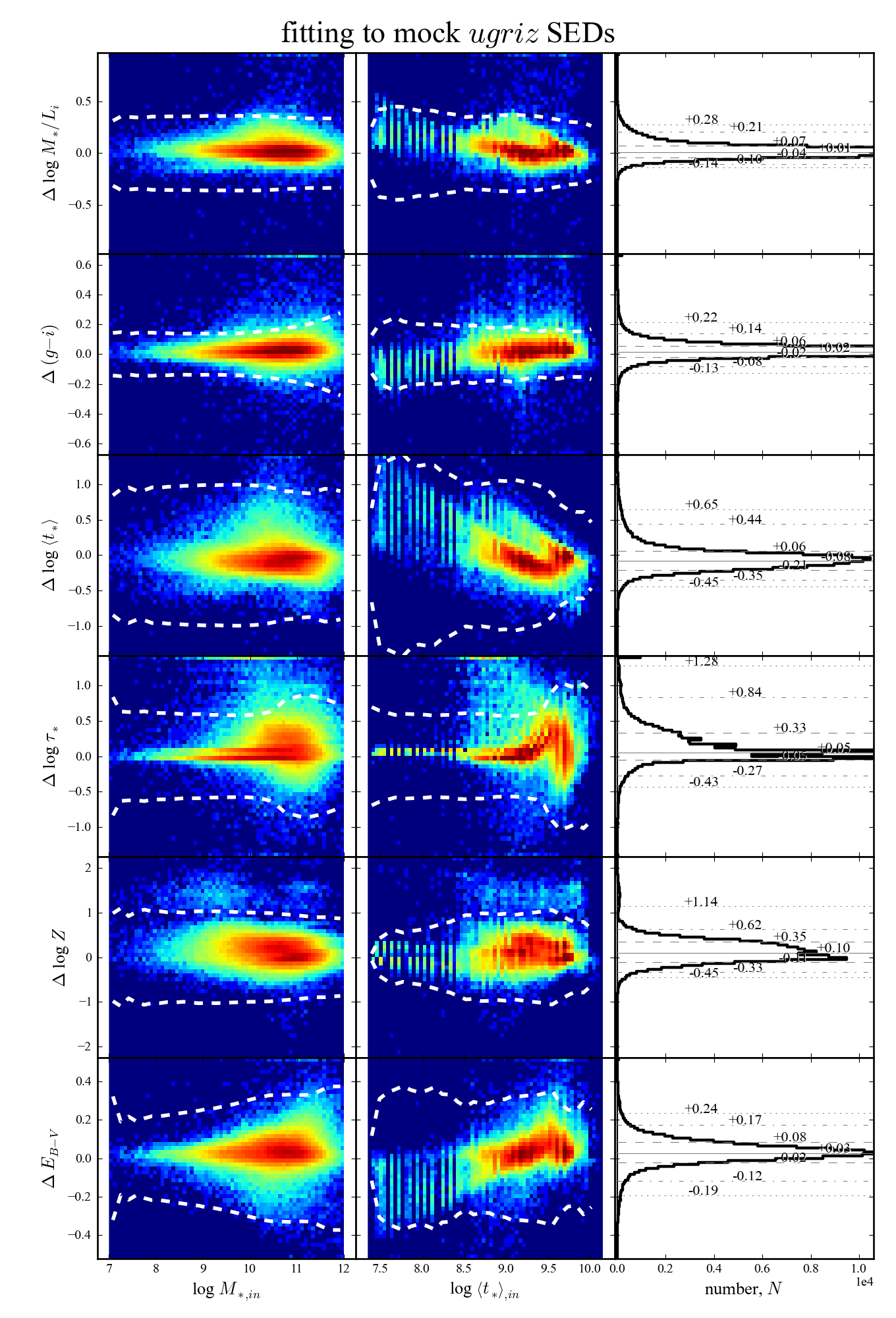
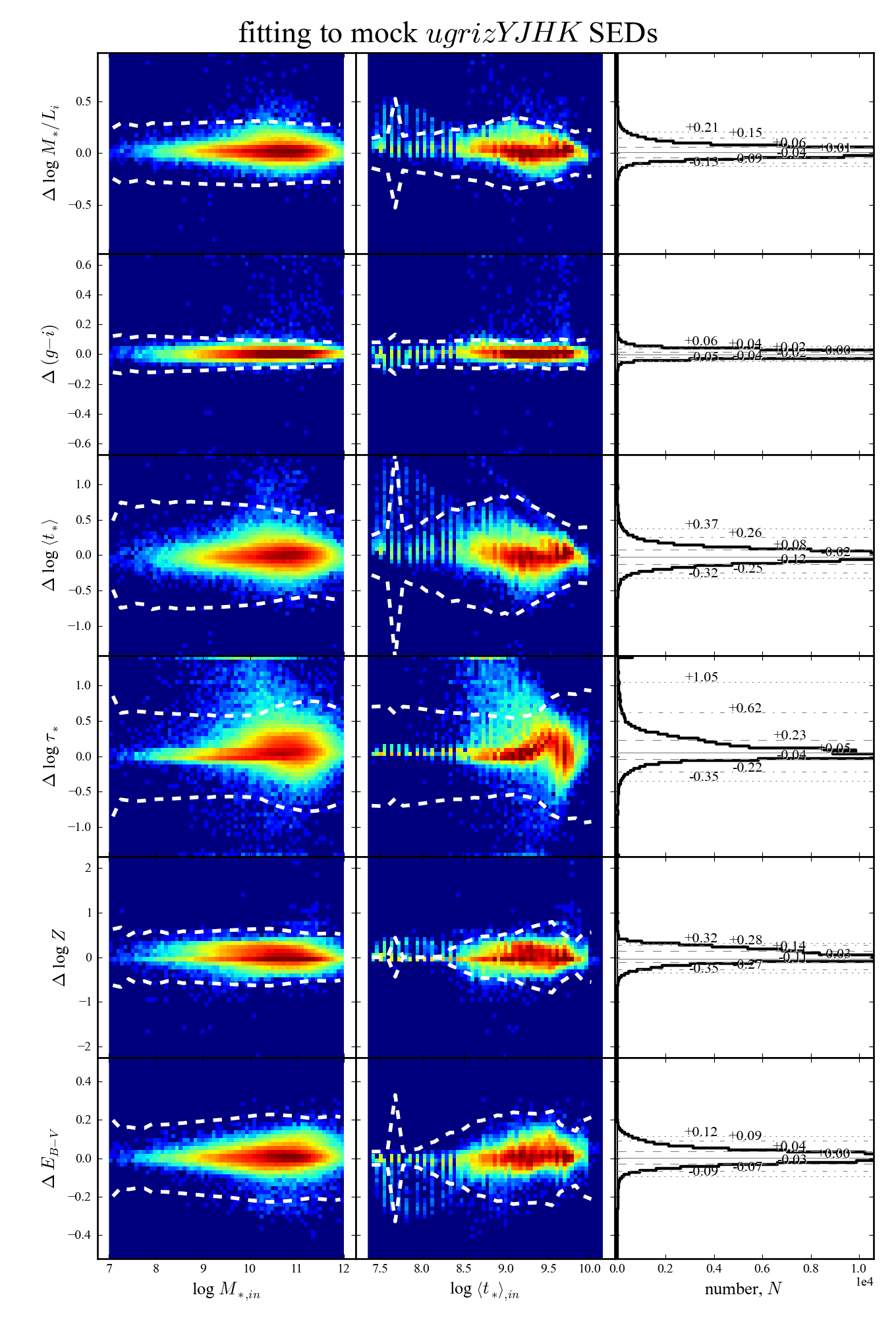
Figure 17: Stellar population parameter recovery for mock galaxy photometry.— These plots are based on the mock galaxy photometry described in Appendix A; each panel shows the difference between the ‘known’ parameter of a mock galaxy and that inferred from a fit to optical–only (left panels) or the optical–plus–NIR (right panels) photometry. In all cases, the ‘$\Delta$’s on the $y$ axes should be understood as ‘recovered–minus–input’; the quantities on the $x$ axes relate to the ‘known’ value. As in Figures 8 and 9, the histograms show the distribution in the ‘$\Delta$’s, with the percentile equivalents of the $\pm 0$/1/2/3$\sigma$ points as marked. In both cases, we are able to recover the SP parameters of the mock galaxies with little to no systematic bias. This is particularly true for $M_{*}/L_{i}$: the reliability of the optical–plus–NIR–derived estimates (median error $\sim 0.05$ dex) is not significantly better than that based on only the optical (median error $\sim 0.06$ dex).

A.1.3 Implications for SED fitting—the subtle role of priors

Given the above, what are we to make of the (very slight) residuals in the $ugriz$ fits? Since we are fitting to the same $ugriz$ photometry in both of the above experiments, the additional information provided by the NIR photometry must exclude some of those models that are consistent with the optical data on its own. In other words, the models allowed by the 5-band fits span a broader range of SP parameter values than those allowed by the 9-band fits; the set of SPL templates allowed by the 5-band fits must be a superset of those allowed by the 9-band fits. (We will look at precisely how the SP parameter estimates change with the inclusion of the NIR data in a moment; for now, let us keep the discussion general.) The implication of this, as is well known, is that an optical SED simply does not encode sufficient information to fully constrain a galaxy’s SP parameters.

Naturally, the models are distinguished by their SED shapes. From the fact that the $ugriz$ fits tend to over-predict the ‘true’ NIR photometry of our mock galaxies, we know that the optical-only fits are consistent with a range of SPL models, and that these models are on average redder than the ‘real’ solution. Now, the fiducial parameter estimate is derived from marginalising over the PDF á la Equation 5. Again, for the optical-only fits, this includes a disproportionally large number of models with the ‘wrong’ SED shape; specifically, models that are substantially too red in the NIR. But these models will also have (very) slightly different optical SED shapes. Hence the very slight offsets seen in the optical bands when the NIR data are excluded.

Consider what would happen if we were to significantly change the form of our assumed priors in such a way as to make these redder fits less likely—for example, by making higher dust extinctions or metallicities less likely than lower ones. Reducing the prior probability of these models directly reduces their contribution to the integral in Equation 5, which defines the Bayesian ‘most likely’ parameter value. This implies that if we were to use more realistic priors, we might be able to do a substantially better job of predicting the NIR photometry based on the optical SEDs. (Parenthetically, this may be why kcorrect is so successful at predicting NIR photometry from optical colours.)

In this context, it is significant that the $ugriz$ residuals seen when fitting only to the optical bands disappear when the NIR data are included. This shows that our SPS algorithm is in fact able to near-perfectly match galaxies’ SEDs given sufficient information, where we have also now shown that ‘sufficient information’ means both optical and NIR photometry. Furthermore, this is possible even despite the fact that the assumed priors are very different from the real distribution intrinsic to the data. These experiments thus suggest that the GAMA optical–plus–NIR dataset can, in principle, be used to constrain galaxies’ SP parameters to the extent that the quality of the fits is not sensitive to the assumed priors. Said another way (and more accurately), so long as NIR data are available, the way that the photometry uncertainties map onto SP parameter space means the allowed range of SP parameters is small enough that the assumption that the priors are locally flat is a good one.

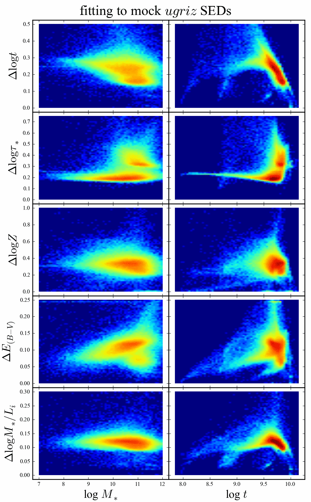
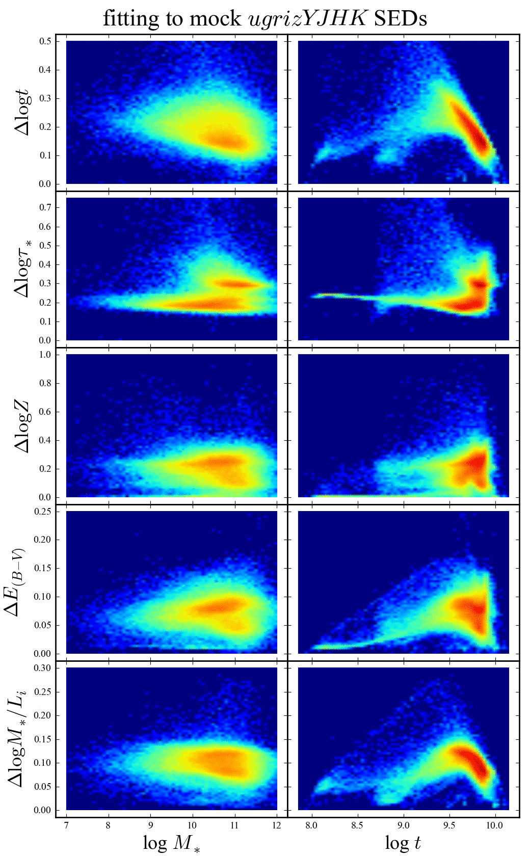
Figure 18: Precision of stellar population parameter estimates for mock galaxies.— In analogy to Figure 4, these plots show the distributions of the formal uncertainties in the inferred SP parameter values for the mock galaxies based either on the optical-only (left panels), or the optical–plus–NIR (right panels) SED fits. If the NIR data are included, the formal uncertainties in the recovered values of all of $t$, $\tau$, $Z$, and $\mathrm{E}_{B\text{-}V}$ are considerably smaller than if they are excluded. However, the formal uncertainties in $M_{*}/L$ are virtually unchanged. By breaking the age–metallicity–dust degeneracies, NIR data provides a better estimate of the ancillary SP parameters, but this has little to no bearing on the precision with which $M_{*}/L$ can be constrained.

As we have already pointed out in §7, there is an important corollary to the idea that we are, in principle, able to near-perfectly match the ‘observed’ SEDs in our mock catalogue. Once NIR data are included, the quality of the fits is no longer limited by the amount of information that is encoded in the data, but instead by how closely the stellar populations that comprise the SPL represent those found in the wild. This means that, to the extent that more complex stellar populations—including more complicated SFHs, a mix of stellar metallicities, and patchy dust geometries—change the shape of a galaxies SEDs, these effects must be adequately folded into the construction of the SPL. In other words, precisely because NIR data provides the additional SP parameter information not found in the optical, robust and reliable fits to optical–plus–NIR SEDs require more sophisticated SPLs (see also §6.2.)

A.2 Parameter recovery

Whereas in the previous section we have focussed on how well our SPS fitting algorithm is able to describe or reproduce the SED shapes of mock galaxies, we now turn to the question of how well galaxies’ SP parameters can be constrained from their broadband SED shapes.

A.2.1 Reliability

In Figure 17, we show how accurately we are able to recover the SP parameters associated with the mock galaxies based either on their optical-only (left panels) or optical–to–NIR (right panels) photometry, and in the face of realistic observational uncertainties. In all cases, the ‘$\Delta$s’ on the $y$ axis should be understood as being the ‘output–minus–input’ parameter value, plotted as a function of the ‘known’, input value from the mock catalogue. As in Figures 8 and 9, the colour-scale shows the logarithmic data density, with the percentile equivalents of the $\pm 0/1/2/3\sigma$ points of the distributions given with the histograms at right.

The first—and, in the context of our main argument, the most crucial—point to be made from these plots is that we are able to recover the $M_{*}/L_{i}$s of the mock galaxies with no discernible bias based on the optical SEDs alone. Further, the $M_{*}/L_{i}$ determinations derived from fits including NIR photometry are not all that much more reliable than those based only on the optical data: on the one hand, the 1 $\sigma$ ‘errors’ are ${}^{+0.07}_{-0.04}$ dex; on the other, they are ${}^{+0.06}_{-0.04}$ dex.

In line with the results of the previous section, where we have shown that our priors tend to over-weight models with redder SED shapes, the optical-only fits imply slightly too-red $(g-i)$ colours. Empirically, the error is $0.015^{+0.057}_{-0.020}$ mag; using the slope of the empirical $(g-i)$–$M_{*}/L_{i}$ relation, this translates to an error of $0.010^{+0.040}_{-0.014}$ dex in $M_{*}/L_{i}$.

For the other SP parameters, as for $M_{*}/L_{i}$, the inclusion of NIR data does not appear to be crucial to obtaining reliable parameter estimates. The median offset between the known and the recovered SP parameter values for the optical–plus–NIR fits is not clearly less than for the optical–only fits. That said, the inclusion of NIR data clearly does reduce the ‘random’ error in the derived SP parameters—that is, the robustness—particularly in the case of $Z$ and $\mathrm{E}_{B\text{-}V}$, as well as $\tau$ for those ‘passive’ galaxies with $t/\tau\gg 1$.

A.2.2 Robustness

The final question to be considered here is how precisely galaxies’ SP parameters can be constrained based on SED fits with or without NIR photometry. We address this question with reference to Figure 18, which shows the distribution of the formal uncertainties in SP parameter estimates derived from the mock photometric catalogues, based on fits to optical–only (left panels) or optical–plus–NIR (right panels) SEDs.

Looking at the global distribution of uncertainties for all galaxies in the mock catalogues, the greatest effect of the NIR is to reduce the uncertainties on $Z$ and on $\left<t_{*}\right>$. The median value of $\Delta\log Z$ goes from 0.35 dex to 0.25 dex with the inclusion of the NIR, while the median value of $\Delta\log\left<t_{*}\right>$ goes from 0.26 dex to 0.19 dex. By comparison, the improvement in $\Delta\log\mathrm{E}_{B\text{-}V}$ is relatively minor: the median value goes from 0.10 dex to 0.07 mag. It is interesting to compare this improvement in $\Delta\log\left<t_{*}\right>$ to that in $\Delta\log t$, which goes from 0.21 to 0.18 dex, and in $\Delta\log\tau$, which remains nearly unchanged at 0.21 dex. This suggests that while NIR photometry helps to break degeneracies between $\left<t_{*}\right>$ and $Z$ (and to a lesser extent $\mathrm{E}_{B\text{-}V}$), and so helps provide a better constraint on instantaneous mean stellar age, it does not provide much additional information concerning the precise SFH.

But again, the NIR data does not lead to a substantial improvement in the accuracy with which $M_{*}/L_{i}$ can be determined: the median value of $\Delta\log M_{*}/L_{i}$ goes from 0.11(4) dex ($\approx 30$ %) to 0.09(8) dex ($\approx 25\%$). The NIR encodes virtually no additional information concerning a galaxy’s stellar mass that cannot be found in the optical.

This fact has one important implication for future stellar mass catalogues. In the previous section, we found that we were able to recover $M_{*}/L_{i}$ for the mock galaxies with an empirical $1\sigma$ ‘error’ on the order of $\pm 0.05$ dex, both with and without the inclusion of NIR data; i.e., more precisely than might be expected from the formal uncertainties of $\pm 0.10$ dex. The reason for this is that, in generating the mock photometry, we have added random photometric errors commensurate with the random photometric errors; in the fitting, on the other hand, we include an error ‘floor’ of 0.05 mag. This error is intended to account for potential differential systematic errors between the different photometric bands. The implication is thus that the accuracy of our stellar mass determinations is not limited by signal–to–noise (i.e., the random observational uncertainties in the photometry in each band), but instead by the relative accuracy of the photometry in the different bands with respect to one another (i.e., differential systematic errors between the different bands). This means that the extent to which the considerably deeper VST and VISTA photometry will improve our ability to constrain galaxies’ stellar masses will depend crucially on how well we are able to control systematic photometric errors in the different bands, including the accuracy of the basic photometric calibrations.

Appendix B Comparisons between GAMA and SDSS

In this Appendix, as a means of validating our stellar mass estimates, we compare them to the latest generation of stellar mass estimates from the MPA-JHU catalogue for SDSS DR7. The motivation for this comparison stems from the fact that the MPA-JHU mass-to-light ratios have been well tested; they thus provide a useful set of benchmark measurements. They are in excellent agreement with other frequently used MPA-JHU mass determinations; e.g., the Kauffmann et al. (2003a) DR4 catalogue. That is, the (SED-derived) DR7 mass estimates are wholly consistent with values derived from spectra. Further, Taylor et al. (2010b) have compared the DR7 MPA-JHU stellar masses to dynamical mass estimates, derived using the Sérsic-fit structural parameters of Guo et al. (2009). Based on the consistency between these stellar mass estimates and dynamical mass estimates, Taylor et al. (2010b) have argued that any differential biases in the stellar-to-dynamical mass ratio as a function of stellar population parameters may be as low as $\lesssim 0.12$ dex ($\sim 40$ %).

There are two facets to this comparison: differences in SDSS and GAMA photometry from which the mass estimates are derived, and differences in the algorithms used to actually derive the mass estimates. We compare the GAMA and SDSS photometry in §B.1. After describing the key differences between the SDSS and GAMA algorithms in §B.2, we will then look at our ability to reproduce the SDSS stellar mass and stellar mass-to-light ratio values using first SDSS model the and then the GAMA auto photometry in §B.3 and §B.4, respectively. In this way, we will hope to identify whether and how these differences affect the derived values for $M_{*}/L$ and $M_{*}$. Before we begin, let us again stress that the rationale behind this comparison is that the SDSS mass-to-light ratios have been well tested; our main concern is thus our ability to reproduce the SDSS values for the galaxies that are common to both SDSS and GAMA.

B.1 Comparing the GAMA and SDSS photometry

The basic SDSS catalogue contains two different photometric measures in each of the $ugriz$ bands. Following the recommendation of Stoughton et al. (2002), it is standard practice to use model photometry to construct multi-band SEDs. This photometry comes from fitting either an exponential or a de Vaucouleurs profile to the observed light distribution. The choice of profile shape and structural parameters (i.e., effective radius, ellipticity, and position angle) are based on the $r$-band image. For the $ugiz$-bands these parameters are then held fixed during fits, so that only overall normalisation is allowed to vary; this is then the model flux. The MPA-JHU mass estimates are based on the model SEDs taken from the basic SDSS catalog.

The second photometric measure is the petro magnitude, which is based on the idea of Petrosian (1976). This flux is measured within a flexible circular aperture, the size of which is based on the observed (radial) surface brightness profile. Again following the recommendations of Stoughton et al. (2002), it is standard practice to use the petro photometry as a measure of total flux. Accordingly, when we consider $\log M_{*}$ below, we will scale the MPA-JHU mass estimates by $-0.4(r_{\texttt{petro}}-r_{\texttt{model}})$ to obtain ‘total’ mass estimates. This is directly analogous to our use of SEDs based on matched aperture auto photometry, scaled to match sersic total magnitudes.

B.1.1 $r$-band Magnitudes

In Figure 19, we compare the different GAMA and SDSS photometric measures of $r$-band flux. This comparison is based on the $\sim 12000$ SDSS-targeted galaxies that appear in the GAMA catalogue. In this Figure, we distinguish between those galaxies whose SDSS model photometry is based on an exponential (blue points) or a de Vaucouleurs (red points) profile.

In each case, it is clear that the relation between different photometric measures depends most strongly on profile shape (parameterised by the GAMA $r$-band derived Sérsic index, $n$). For $n\gtrsim 2$, the difference between the GAMA Sérsic-fit and SDSS petro fluxes is more or less as expected: the fraction of missed flux increases rapidly from $\approx 0$ for $n\sim 2$, to $\approx$ 0.1 mag for $n\approx 4$ galaxies, to $\approx 0.5$ mag for $n\approx 8$, and so on.

The most striking feature of Figure 19 is the large $n$-dependent differences between the SDSS model and GAMA sersic and auto photometry. The crucial assumption behind the SDSS model photometry is that galaxies can be well described by a Sérsic profile with either $n=1$ or $n=4$. For those galaxies with a GAMA-derived $n\approx 1$, the results in Figure 19 suggest that the GAMA sersic photometry may miss $\lesssim 10$ % ($\lesssim 0.04$ dex) of the flux for low $n$ galaxies; for galaxies with $n\approx 4$, there is excellent agreement between the GAMA sersic and SDSS model photometry.

Away from these points, however, the model photometry has large systematic biases: for both exponential- and de Vaucouleurs–like galaxies, where the model Sérsic index ($n=1$ or $n=4$) is higher than the ‘true’ value, the model flux significantly over-estimates the ‘true’ total flux. For exponential-like galaxies, the size of the differential effect is nearly 0.3 mag between $n\approx 0.5$ and $n\approx 2$; for de Vaucouleurs-like galaxies, the effect is greater than 0.7 mag (a factor of 2!) between $n\approx 2$ and $n\approx 8$. This is thus a major, if not the largest, source of error in the SDSS mass estimates.

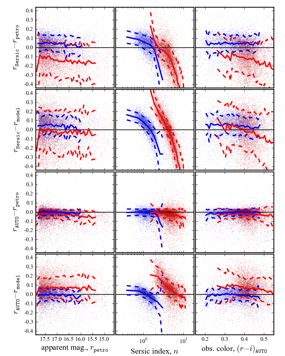
Figure 19: Comparison between GAMA and SDSS $r$-band magnitude measurements.— Each panel of this Figure shows the difference between a GAMA and an SDSS measure of $r$-band magnitude as a function of (left to right) apparent magnitude, GAMA-derived Sérsic index, $n$, or observed colour. Within each panel, we make the distinction between those objects that are fit using an exponential profile (blue) or a de Vaucouleurs profile (red) for the SDSS model photometry. For GAMA, we use auto magnitudes to construct multicolour SEDs, and the $r$-band sersic magnitude to measure total flux; it is standard SDSS practice to use model magnitudes for SEDs, and the petro magnitude as a measure of total flux. As expected, the petro magnitude misses an increasingly large fraction of total flux for galaxies with higher values of $n$. It seems that the GAMA sersic magnitude may miss up to $\lesssim 10$ % of flux for $n\lesssim 2$ galaxies. The SDSS model magnitudes (which assume either $n=1$ or $n=4$) have strong $n$-dependent systematics: where the assumed value of $n$ in the model underestimates the ‘true’ value of $n$, the model flux overestimates the total magnitude by up to $\sim 0.3$ mag. Between $n\sim 2.5$ and $n\sim 8$, the size of the differential effect for de Vaucouleurs-like galaxies is greater than a factor of 2.

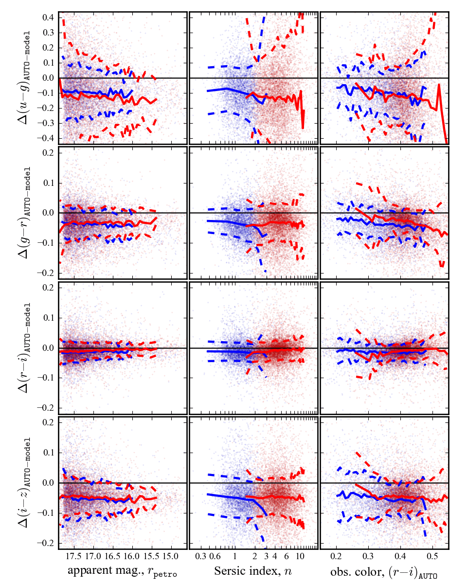
Figure 20: Comparison between GAMA AUTO and SDSS model photometry.— Each row shows the difference in the measured, observers’ frame colours of galaxies as reported in the GAMA and SDSS catalogues; the ‘$\Delta$’ should be understood as meaning GAMA–minus–SDSS. From left to right, the panels show the systematic differences in observed colour as a function of apparent magnitude, Sérsic index, and $(r-i)$ colour. As in Figure 19, we make the distinction between those objects that are fit using an exponential profile (blue) or a de Vaucouleurs profile (red) for the SDSS model photometry. The points show the data themselves; the lines show the binned biweight mean and scatter. The SDSS model SEDs are systematically redder than the GAMA auto ones: the cumulative difference in $(u-z)$ is 0.2 mag. Note that we find no such systematic differences between the GAMA auto and SDSS petro colours. This suggests that the SDSS data may be better analysed using petro rather than model SEDs.

B.1.2 $ugriz$ SEDs

In Figure 20, we show a comparison between galaxies’ optical colours as reported in the GAMA and SDSS catalogues. Although the current GAMA optical photometry is derived from the SDSS imaging data, there are systematic differences between the galaxy colours—as measured using the GAMA AUTO and SDSS model photometry—that are used as the basic inputs to the stellar mass estimation calculation.

In comparison to the GAMA AUTO photometry, the SDSS model SEDs are systematically redder across all bands. Quantitatively, the observed ‘GAMA auto–minus–SDSS model’ offsets are $\Delta(u-g)=-0.10$ mag, $\Delta(g-r)=-0.03$ mag, $\Delta(r-i)=-0.01$ mag, and $\Delta(i-z)=-0.05$ mag; the cumulative offset between $u$ and $z$ is thus $-0.2$ mag. These offsets are not a strong function of apparent brightness. Particularly for the bluer bands, they may depend weakly on Sérsic index. Further, looking at the right-hand panels of this Figure, there is the hint that the offsets vary systematically with observed colour: this immediately suggests that colour gradients may play a role in one or the other of these measurements.

Note that we find no such systematic offsets between the GAMA auto and SDSS petro colours. That is, whatever the cause of the discrepancies seen in Figure 20, it is specific to the SDSS model photometry. We also note that the fact that the model photometry is so sensitive to $n$ implies that model-derived SEDs may be badly biased by colour gradients: a small change in Sérsic index across different bands will produce a relatively large differential bias in the inferred fluxes. Taken together, these two points suggest that that when using SDSS photometry, despite the fact that the petro photometry is not PSF-matched, it may provide a better basis for constructing multi-colour SEDs than model photometry.

B.2 Differences between the MPA-JHU and GAMA mass estimation algorithms

Unlike previous MPA-JHU catalogues (e.g. Kauffmann et al., 2003a; Brinchmann et al., 2004; Gallazzi et al., 2005) that were based on the SDSS spectroscopy, the DR7 MPA-JHU stellar mass estimates are based on fits to the $ugriz$ photometry. The first difference between the MPA-JHU and GAMA algorithms is that for the MPA-JHU mass estimates, the observed photometry has been corrected for contributions from emission lines (which are not included in the BC03 models), under the assumption that the global emission line contribution is the same as in the spectroscopic fiber aperture.

Like the one described here, the MPA-JHU SPL is based on the BC03 SSP models, and assuming a Chabrier (2003) IMF. Whereas we use a Calzetti et al. (2000) dust law, however, the SDSS SPL spectra use the Charlot & Fall (2000) curve to account for dust obscuration. At least in terms of the values of $M_{*}/L$, as we shall show, this difference is not important.

The biggest structural difference between the GAMA and SDSS stellar mass calculations is that, whereas we have constructed our SPL by sampling a semi-regular grid in ($t,~{}\tau,~{}Z,~{}\mathrm{E}_{B\text{-}V}$) parameter space, the MPA-JHU masses are based on a library made up of large number of Monte Carlo realizations of different star formation histories. The priors in the MPA-JHU algorithm are applied in the Monte Carlo sampling of the allowed parameter space (see also Gallazzi et al., 2005). Specifically, the model ages are randomly sampled from a uniform distributions in both formation time (over the range $1.5<t_{\mathrm{form}}/[\mathrm{Gyr}]<13.5$) and in the exponential decay rate ($0<\gamma/[\mathrm{Gyr}^{-1}]<1$; here, $\gamma$ can be thought of as $1/\tau$). The models also include a number of secondary bursts of star formation. The burst probabilities are normalised such that 10 % of galaxies experience a burst in the last 2 Gyr, with the burst times uniformly distributed between $t_{\mathrm{form}}$ and and the time of observation. Individual bursts are treated as constant star formation rate events lasting for $10^{7.5}$—$10^{8.5}$ yr. The strength of each burst is parameterised by the mass relative to the ‘underlying’ population, which is logarithmically distributed between $0.03<f_{M_{*},\mathrm{burst}}<0.4$. Finally, the assumed metallicity prior is logarithmic for super-solar metallicites, with lower metallicites downweighted through an assumed prior distribution of the form $(\log Z)^{1/3}$ for $0.02<Z<0.2$. The prior distribution of dust extinctions is derived from the SDSS H$\alpha$/H$\beta$ ratios (Jarle Brinchmann, private communication; 24/09/2009). In terms of their SPLs, the major differences between the MPA-JHU and GAMA calculations are thus the inclusion of bursts, and the different form of the metallicity distribution prior.

The decision to randomly sample parameter space, rather than to use a (semi-)regular grid has two consequences. First, it makes it possible to accommodate bursts in the SPL (as described above); this would not be computationally practical to include into a SPL grid like ours, since it would expand the parameter space by (at least) an additional three dimensions. Second, the nominal SDSS parameter values given in the MPA-JHU catalogues are the median of the posterior probability distribution; i.e., the 50 % confidence upper/lower limits, rather than the ‘most likely’ value from explicit marginalisation over the PDF. That said, at least for the GAMA mass estimates, we find that the (probability weighted) median and mean values of $M_{*}/L$ are in extremely good agreement. This implies, albeit weakly, that the posterior probability distributions for $M_{*}/L$ are roughly symmetric about the mean/median value.

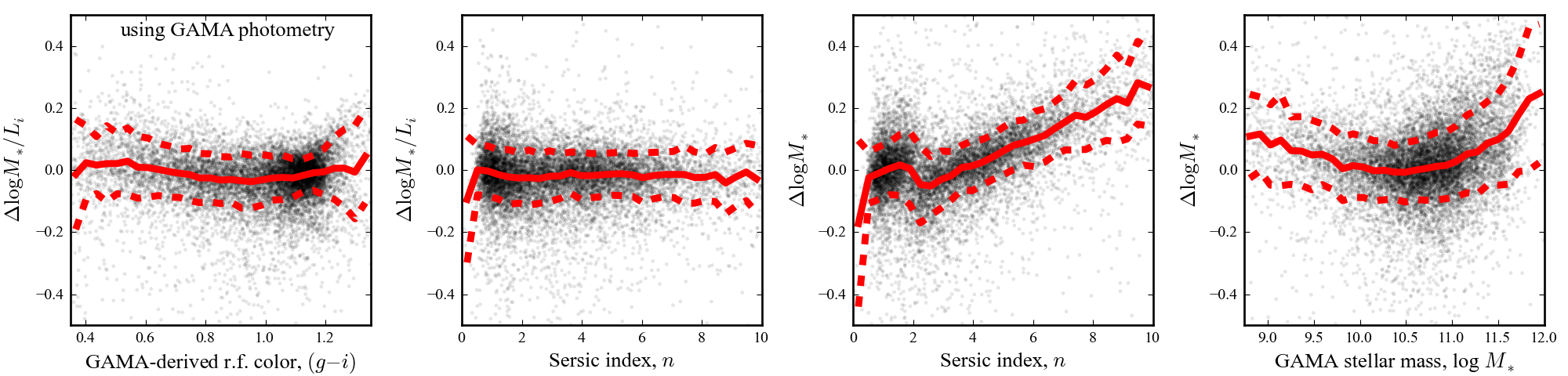
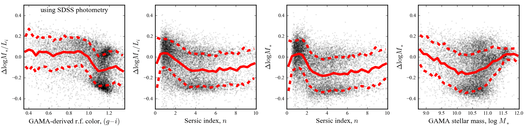
Figure 21: Stellar mass-to-light ratios and stellar masses inferred from SDSS model and GAMA AUTO photometry.— In the lower panels, the ‘GAMA-derived’ values are based on SEDs constructed from the SDSS model photometry; in the upper panels, the ‘GAMA’ values are derived from the GAMA auto SEDs. In each case, the ‘$\Delta$’s should be understood as GAMA-minus-SDSS. Using the SDSS model photometry, we do not do a particularly good job at reproducing the (well-tested) SDSS-derived values of $M_{*}/L$; using the GAMA auto photometry, the agreement is very good (the reasons for this are discussed at greater length in §B.1.2 and §B.4). While the fiducial GAMA $M_{*}/L$s agree very well with those from SDSS, the GAMA masses are systematically larger than the SDSS values. This can only be explained by missed flux in the SDSS model photometry. For the highest values of $n$ and $M_{*}$, GAMA finds $\gtrsim 0.15$ dex more light/mass than SDSS (see also §B.1.1 and Figure 19).

B.3 Comparison between the MPA-JHU- and GAMA-derived mass estimates I. Using GAMA auto SEDs

How well are we able to reproduce the MPA-JHU values for $M_{*}/L$ and $M_{*}$? We address this question in Figure 21. In the left-hand panels of this Figure, we compare the stellar masses that we derive based on SDSS photometry to those given in the MPA-JHU catalogue: these panels thus probe differences in the GAMA and SDSS algorithms applied to the same data. In the upper panels of this Figure, we compare our fiducial stellar mass estimates based on GAMA photometry. It is thus these panels that most interest us, inasmuch as these panels show a direct comparison between the well-tested MPA-JHU values and our own.

Looking at the upper panels of Figure 21, the agreement between our fiducial mass estimates and the MPA-JHU values is very good: the random scatter between the two values of $M_{*}/L$ is small, and there are no obvious systematics. More quantitatively, our AUTO-derived $M_{*}/L$s agree with the MPA-JHU values with a biweight mean and scatter in $\Delta M_{*}/L$ of $-0.01$ and $0.07$ dex, respectively. The offsets in $M_{*}/L$ as a function of restframe colour are at the level of a few percent ($\lesssim 0.02$ dex). That said, there are large differences in the total inferred $M_{*}$ as a function of $n$. Given that we can faithfully reproduce the $M_{*}/L$s, this discrepancy can only be explained by differences in the total $L$s. These results thus suggest that missed flux is a significant problem in the MPA-JHU SDSS masses.

B.4 Comparison between the MPA-JHU- and GAMA-derived mass estimates II. Using SDSS model SEDs

While we have now shown very good agreement between the MPA-JHU- and GAMA-derived $M_{*}/L$s for SDSS galaxies, the comparison presented in the previous Section mixes the effects of differences in both the input photometry and the mechanics of the stellar mass estimation algorithms. The next obvious question is how well the two algorithms agree when applied to the same data.

Looking at the lower panels of Figure 21, it is clear that we do not do a particularly good job of reproducing the MPA-JHU masses when using the SDSS model photometry to construct galaxy SEDs. We see mild systematic differences between the GAMA- and SDSS-derived values of $M_{*}/L$ as a function of both colour and structure, and the random scatter between the two estimates is not small: $\sim 0.15$ dex. Further, there is a distinct population of de Vaucouleurs-like galaxies ($n\sim 2.5$–6) galaxies with rest frame $(g-i)$ colours of $\sim 1.1$ whose GAMA-derived $M_{*}/L$s are lower by $\sim 0.25$ dex.

How can it be that we do a better job at reproducing the MPA-JHU $M_{*}/L$s when using the GAMA photometry than we do using the SDSS model photometry? At least part of the answer is thus directly tied to differences between the SDSS model and GAMA auto photometry. We have made similar comparisons using SDSS petro photometry. Perhaps unsurprisingly, given the close agreement between the petro and auto colours, we do not find any strong systematic differences between the GAMA- and SDSS-derived values in this case. The median value of $\Delta M_{*}/L_{i}$ is $-0.02$ dex; the RMS $\Delta M_{*}/L_{i}$ is 0.11 dex. There are no obvious trends in $\Delta M_{*}/L_{i}$ with apparent magnitude, Sérsic index, or inferred rest-frame colour. That is, the problem appears to be specific to the SDSS model photometry.

We have seen that the SDSS model SEDs are systematically redder than those constructed using GAMA auto magnitudes. The effect of these differences can be understood by looking at Figure 1. Using the model SEDs, the ‘problem’ objects (that is, those galaxies where there are large differences in the GAMA- and SDSS- derived stellar mass estimates) prefer templates with young ages ($\left<t_{*}\right>\lesssim 3$ Gyr), high metallicity ($Z\approx 0.05$; the highest value allowed in our BC03 library) and moderately heavy dust extinction ($\mathrm{E}_{B\text{-}V}\sim 0.2$). When using the GAMA AUTO photometry, these objects come out to be considerably older ($\left<t_{*}\right>\sim 6$ Gyr), lower metallicity ($Z\sim 0.01$) and less dusty ($\mathrm{E}_{B\text{-}V}\sim 0.05$—0.10).

Looking carefully at the $1.0<(g-i)<1.2$ region of Figure 1, one can see that immediately above the broad strip defined by the older, low-SSFR models (colour-coded red in the upper-left panel), there is a narrower strip of models with ages $\left<t_{*}\right>\sim 1$ Gyr (colour-coded green). In the lower-lefthand panel of Figure 1, these models can also be seen to have $Z=0.05$ (colour-coded red). Note that this is precisely the regime where we see the largest differences in the GAMA- and MPA-JHU-derived $M_{*}/L$s.

This explains the differences between our stellar mass estimates based on the auto and model photometry: the 0.13 mag offset in $(u-r)$ between the model and auto photometry pushes these galaxies up towards the upper edge of the region of colour space spanned by the models. The redder $(u-r)$ model colours thus open up a qualitatively different, young, high-metallicity stellar population solution for what would otherwise be old, lower-metallicity galaxies.

But how is it that the SDSS stellar mass estimates, which are based on the ‘wrong’ model SEDs still get the ‘right’ value for $M*/L$? We speculate that the answer may lie in the different metallicity and/or dust priors used by the MPA-JHU team. The priors most strongly affect galaxies with low metallicities and dust extinction (Jarle Brinchmann, private communication; 24/09/2009); these are precisely the kinds of galaxies where we see the greatest discrepancies between the GAMA- and MPA-JHU-derived values of $M_{*}/L$. That is, it would seem that the ‘problem’ dustier, younger, and high-metallicity solutions preferred by the model photometry are down-weighted by the inclusion of a dust prior in the MPA-JHU algorithm. Here, too, the SDSS decision to use the median, rather than the mean, of the PDF will help to reduce any susceptibility to a ‘bimodality’ in the PDF, and so reduce the likelihood of choosing these ‘problem’ solutions. In our case, using the GAMA auto photometry, the inclusion of such a prior is unnecessary.

Again, our primary motivation for performing this comparison is to test our ability to reproduce the well tested MPA-JHU values for $M_{*}/L$. Given that we have demonstrated our ability to do so using our own $ugriz$ photometry, and the fact that without access to the MPA-JHU algorithm we are unable to perform any more detailed tests or comparisons, we have not investigated this issue any further.

B.5 Summary

In this Appendix, we have compared the GAMA photometry and stellar mass estimates to those from SDSS. Our primary motivation for this comparison is that is has been argued, based on their consistency with dynamical mass estimates, the SDSS stellar mass estimates have no strong systematic differential biases for galaxies with different stellar populations (Taylor et al., 2010b). When using the GAMA photometry, we find excellent agreement between our fiducial estimates of $M_{*}/L$s and those from SDSS, with no strong differential biases as a function of mass, colour, or structure. This argues against there being any strong biases in the GAMA $M_{*}/L$ estimates. We will investigate this further through comparison between the GAMA stellar and dynamical mass estimates in a separate work.

We have also shown that there are significant differences between the GAMA and SDSS estimates of total flux, which come from sersic and model photometry, respectively. These differences are a strong function of $n$: for $n=1$ and $n=4$ galaxies, where the SDSS model assumes the ‘right’ value of $n$, we find excellent agreement between the two surveys’ photometry. Away from these points, however, the model photometry is strongly biased. For de Vaucouleurs-like galaxies, the size of the differential bias in the model photometry is as large as a factor of 2. This will have a significant impact on a number of stellar mass-centric measurements like the mass function or the size–mass relationship.

We have shown that there are significant systematic differences between the GAMA- and SDSS-derived colours, which are derived from auto and model photometry, respectively. The SDSS model photometry is systematically redder, with a net offset of $\Delta(u-z)=0.2$ mag. We suggest that it may be better to use petro, rather than model photometry when analysing SDSS data: we find no such differentials between the GAMA auto and SDSS petro photometry . When we apply our SPS pipeline to the model photometry, our stellar mass estimates no longer agree well with those from SDSS. We suggest that these differences may be explained by the different priors used in the SDSS pipeline, which act to downweight young, moderately dusty, and high metallicity SPS fits. In the case of SDSS, their priors would seem to effectively circumvent the potential biases in $M_{*}/L$ that these photometric biases might produce. In our case, we are able to reproduce the well-tested SDSS values with no need for such priors.

References

- Abazajian et al. (2009) Abazajian K V et al., 2009, ApJS 182, 543
- Adelman-McCarthy et al. (2009)
- Baldry et al. (2006) Baldry I K, Balogh M L, Bower R G, Glazebrook K, Nichol R C, Bamford S P, Budavari T, 2006, MNRAS 373, 469
- Baldry et al. (2010) Baldry I K, Robotham A S G, Hill D T, Driver S P, Liske J, Norberg P et al., 2010, MNRAS 404, 86
- Baldry et al. (in prep.)
- Bell & de Jong (2001) Bell E F, de Jong R S, 2001, ApJ 550, 212
- Bell et al. (2003) Bell E F, McIntosh D H, Katz N, Weinberg M D, 2003, ApJS 149, 289
- Benitez (2000) Benitez N, 2000, AJ 536, 571
- Bertin & Arnouts (1996) Bertin E & Arnouts S, A&A 117, 393
- Blanton et al. (2005) Blanton M R, Eisenstein D, Hogg D W, Schlegel B K, Brinchmann J, 2005, ApJ 629, 143
- Blanton & Roweis (2007) Blanton M R & Roweis S, 2007, ApJ 133, 734
- Brammer et al. (2008) Brammer G B, Van Dokkum P G, Coppi P, 2008, ApJ 686, 1503
- Brinchmann & Ellis (2000) Brinchmann J & Ellis R S, 2000, ApJ 536, L77
- Brinchmann et al. (2004) Brinchmann J, Charlot S, White SDM, Tremonti C, Kauffmann G, Heckman T, Brinkmann J, 2004, MNRAS 351, 1151
- Bruzual (1993) Bruzual G, 1993, ApJ 273, 105
- Brough et al. (2011) Brough S et al., MNRAS 413, 1236
- Bruzual (2007) Bruzual G, 2007, astro-ph/0703052
- (18) Bruzual G & Charlot S, 2003, MNRAS 344, 1000
- Calzetti et al. (2000) Calzetti D, Armus L, Bohlin R C, Kinney A L, Koorneef J, Storchi-Bergmann T, 2000, ApJ 533, 682
- Carter et al. (2009) Carter D, Smith D J B, Percival S M, Baldry I K, Collins C A, James P A, Salaris M, Simpson C, Stott J P, Mobasher B, 2009, MNRAS 397, 695
- Chabrier (2003) Chabrier G, 2003, ApJ 586, L133
- Cimatti et al. (2008) Cimatti A, Cassata P, Pozzetti L, Kurk J, Mignoli M, Renzini A, Daddi E, Bolzonella M, Brusa M, Rodighiero G, Dickinson M, Franchesini A, Zamorani G, Bert S, Rosati P, Halliday C, 2008, A&A 481, 21
- (23) Charlot S & Bruzual G, 2007
- Charlot & Fall (2000) Charlot S & Fall S M, 2000, ApJ 539, 718
- Cole et al. (2001) Cole S, Norberg P, Baugh C M, Frenk C S, 2001, MNRAS 326, 255
- Cole et al. (2005) Cole S, Percival W J, Peacock J A, Norberg P, Baugh C M, Frenk C S, 2005, MNRAS 362, 505
- Colless et al. (2001) Colless M, Dalton G, Maddox S, Sutherland W, Norberg P et al., 2001, MNRAS 328, 1039
- Colless et al. (2003) Colless M, Peterson B A, Jackson C, Peacock J A, Cole S, Norberg P et al., 2003, arXiv:astro-ph/0306581
- Conroy, Gunn & White (2009) Conroy C, Gunn J E, White M, 2009, ApJ 699, 486
- Conroy & Gunn (2010) Conroy C & White M, 2010, ApJ 712, 833
- Conti et al. (2003) Conti A et al., 2003, AJ 126, 2330
- Cutri et al. (2003) Cutri R M, Skrutskie M F, Van Dyke S, et al., 2003, ‘Explanatory Supplement to the 2MASS All Sky Data Release and Extended Mission Products’, NASA/IPAC Infrared Science Archive, http://www.ipac.caltech.edu/2mass/releases/allsky/doc/
- Davis et al. (2003) Davis M, Faber S M, Newman J, Phillips A C, Ellis R S, Steidel C C et al., 2003, Proc. SPIE 4834, 161
- Djorgovsky & Davis (1987) Djorgovsky S & Davis M, 1987, ApJ 313, 59
- Doi et al. (2010) Doi M et al., 2010, AJ 139, 1628
- Dressler (1980) Dressler A, 1980, ApJ 313, 42
- Dressler et al. (1987) Dressler A, Lynden-Bell D, Burstein D, Davies R L, Faber S M, Terlevich R, Wegner G, 1987, ApJ 313, 42
- Driver et al. (2011) Driver S P, Hill D T, Kelvin L S, Robotham A S G, Liske J, Norberg P, Baldry I K, Bamford S P, Hopkins A M, Loveday J, Peacock J A, et al., 2011, MNRAS 413, 971
- Driver et al. (2005) Driver S P, Liske J, Cross N J G, De Propris R, Allen P D, 2005, MNRAS 360, 81
- Driver et al. (2009) Driver S P, Norberg P, Baldry I K, Bamford S P, Hopkins A M, Liske J, Loveday J, Peacock J A, 2009, A&G 50, 5.12
- Driver et al. (2007) Driver S P, Popescu C C, Tuffs R J, Liske J, Graham A W, Allen P D, de Propris R, 2007, MNRAS 379, 1022
- Dye et al. (2006) Dye S, Warren S J, Hambly N C, Cross N J G, Hodgkin S T, Irwin M J, Lawrence A et al., 2006, MNRAS 372, 1227
- Eales et al. (2010) Eales S, Dunne L et al., 2010, PASP 122, 499
- Faber & Jackson (1976) Faber S M & Jackson R E, 1976, ApJ 204, 668
- Fischera & Dopita (2005) Fischera J & Dopita M, 2005, ApJ 619, 340
- Gallazzi et al. (2005) Gallazzi A, Charlot S, Brinchmann J, White S D M, Tremonti C A, 2005, MNRAS 362, 41
- Gallazzi et al. (2006) Gallazzi A, Charlot S, Brinchmann J, White S D M, 2006, MNRAS 370, 1106
- Gallazzi & Bell (2009) Gallazzi A & Bell E F, 2009, ApJS (accepted; arXiv:0910.1591)
- Gunawardhana et al. (2011) Gunawaradhana M et al., 2011, MNRAS (accepted; arXiv:1104.2379)
- Guo et al. (2009) Guo Y, McIntosh D H, Mo H J, Katz N, van den Bosch F C, Weinberg M, Weinmann S M, Pasquali A, Yang X, 2009, MNRAS 398 1129
- Hambly et al. (2008) Hambly N C et al., 2008, MNRAS 384, 637
- Heavens, Jiminez & Lahov (2000) Heavens A, Jiminez R & Lahov O, 2000, MNRAS 317, 965
- Hewett et al. (2006) Hewett P C, Warren S J, Leggett S K, Hodgkin S T, 2006, MNRAS 367, 454
- Hill et al. (2010) Hill D T, Kelvin L S, Robotham A S G, Liske J, Norberg P, Baldry I K, Bamford S P, Hopkins A M, Loveday J, Peacock J A et al., 2010, MNRAS (submitted; arXiv:1009.0614v1)
- Hodgkin et al. (2009) Hodgkin S T, Irwin M J, Hewett P C, Warren S J, 2009, MNRAS 394, 675
- Hogg et al. (2002) Hogg D W, Baldry I K, Blanton M R, Eistenstein D J, 2002, astro-ph/0210394v1
- Im et al. (2002) Im M et al., 2002, ApJ 571, 136
- Jones et al. (2009) Jones D H, Read M A, Saunders W, Colless M, Jarrett T, Parker Q A, Fairall A P, Mauch T, Sadler E, Watson F G et al., 2009, MNRAS 399, 683
- Jones et al. (2004) Jones D H, Saunders W, Colless M, Read M A, Parker Q A, Watson F G et al., 2004, MNRAS 355, 747
- Kannappan & Gawiser (2007) Kannappan S J & Gawiser E, 2007, ApJ 657, L5
- Kauffmann et al. (2003a) Kauffmann G, Heckman T M, White S D M et al., 2003, MNRAS 341, 33
- Kauffmann et al. (2003b) Kauffmann G, Heckman T M, White S D M et al., 2003, MNRAS 341, 54
- Kauffmann et al. (2004) Kauffmann G, White S D M, Heckman T M, Ménard B, Brinchmann J, Charlot S, Tremonti C, Brinkmann J, 2004, MNRAS 353, 713
- Kelvin et al. (in prep.)
- Kriek et al. (2010) Kriek M, Labbé I, Conroy C, Whitaker K E, van Dokkum P G et al., 2010, ApJ, 722, L64
- Kron et al. (1980) Kron R G, ApJS 43, 305
- Lanyon-Foster et al. (2007) Lanyon-Foster M M, Conselice C J, Merrifield M R, 2007, MNRAS 380, 571
- Lawrence et al. (2007) Lawrence A, Warren S J, Almaini O, Edge A C, Hambly N C, Jameson R F, Lucas P, Casali M, 2007, MNRAS 379, 1599
- Le Borgne & Rocca-Volmerange (2002) Le Borgne D & Rocca-Volmerange B, 2002, A&A 386, 466
- Le Fèvre et al. (2005) Le Fèvre O, Vettolani G, Garilli B, Tresse L et al., 2005, A&A 439, 845
- Leitherer et al. (1999) Leitherer C, Schaerer D, Goldader J D, González Delgado R M, Robert C, Kune D F, de Mello D F, Devost D, Heckman T M, 1999, ApJS 123, 3
- Lilly et al. (2007) Lilly S J, Le Fèvre O, Renzini A, Zamorani G, Scodeggio M et al., ApJS 172, 70
- Liske et al. (2003) Liske J, Lemon D J, Driver S P, Cross N J G, Couch W J, 2003, MNRAS 344, 307
- Liske et al. (in prep.)
- Loveday et al. (in prep.)
- (76) Maraston C, 2005, MNRAS 362, 799
- Maraston (2006) Maraston C, Daddi E, Renzini A, Cimatti A, Dickinson M, Papovich C, Pasquali A, Pirzkal N, 2006, ApJ 652, 85
- Martin et al. (2005) Martin D C, Fanson J, Schiminovich D, Morrissey P, Friedman P G et al., 2005, ApJ 619 L1
- Minkowski (1962) Minkowski R, 1962, in Problems of Extragalactic Research (IAU Symp. 15), G C McVittie, ed. (Macmillan, New York)
- Morrissey et al. (2007) Morrissey P, Conrow T, Barlow T A, Small T, Seibert M, Wyder T, Budavári T, 2007, ApJS 173, 682
- Muzzin et al. (2009) Muzzin A, Marchesini D, van Dokkum P G, Labbé I, Kriek M, Franx M, 2009, ApJ701, 1839
- Nicol et al. (2010) Nicol M-H, Meisenheimer K, Wolf C, Tapken C, 2010, ApJ (accepted; arXiv:1011.4067v1)
- Panter, Heavens & Jiminez (2003) Panter B, Heavens A F, Jimenez R, 2003, MNRAS 343, 1145
- Percival et al. (2009) Percival S M, Salaris M, Cassisi S, Pietrinferni A, 2009, ApJ 690, 427
- Peng et al. (2002) Peng C Y, Ho L C, Impey C D, Rix H-W, 2002, AJ 124, 266
- Petrosian (1976) Petrosian V, ApJ 210, L53
- Popescu et al. (2000) Popescu C C, Misiriotis A, Kylafis N D, Tuffs R J, Fischera J, 2000, A&A 362, 138
- Pozetti et al. (2007) Pozzetti L et al., 2007, A&A 474, 443
- Robotham et al. (2010) Robotham A, Driver S P, Norberg P et al., 2010, PASA 27, 76
- Sandage & Visvanathan (1978) Sandage A & Visvanathan N, 1978, AJ 225, 742
- Saunders et al. (2004) Saunders W, Bridge T, Gillingham P, Haynes R, Smith G, Whittard J D et al., 2004, SPIE 5492, 389
- Scoville et al. (2007) Scoville N J et al., 2007, ApJS 172, 1
- Sharp et al. (2006) Sharp R, Saunders W, Smith G et al., 2006, SPIE 6269, 14
- Shen et al. (2003) Shen S, Mo H J, White S D M, Blanton M R, Kauffmann G, Voges W, Brinkmann J, Csabai J, 2003, MNRAS 343, 978
- Skrutskie et al. (2006) Skrutskie M F, Cutri R M, Stiening R, Weinberg M, Schneider S, Carpenter J M, et al., 2006, ApJ 131, 1163
- Stoughton et al. (2002) Stoughton C et al., 2002, AJ 123, 485
- Strateva et al. (2001) Strateva I et al., 2001, AJ, 122, 1861
- Strauss et al. (2002) Strauss M A, Weinberg S H, Lupton R H, Narayanan V K et al., 2002, AJ, 124, 1810
- Taylor et al. (2009) Taylor E N, Franx M, van Dokkum P G, Bell E F, Brammer G B, Rudnick G, Wuyts S, Gawiser E, Lira P, Urry C M, Rix H-W, 2009, ApJ 694, 1171
- Taylor et al. (2010a) Taylor E N, Franx M, Glazebrook K, Brinchmann J, van der Wel A, van Dokkum P G, 2010a, ApJ 720, 723
- Taylor et al. (2010b) Taylor E N, Franx M, Brinchmann J, van der Wel A, van Dokkum P G, 2010b, ApJ 722, 1
- Tinsley & Gunn (1976) Tinsley B M & Gunn J E, 1976, ApJ 203, 52
- Tinsley (1978) Tinsley B M, 1978, ApJ 222, 14
- Tojeiro et al. (2008) Tojeiro R, Heavens A F, Jiminez R, Panter B, 2007, MNRAS 381, 1252
- Tonry et al. (2000) Tonry J L, Blakeslee J P, Ajhar E A, Dressler A, 2000, ApJ 530, 625
- Tremonti et al. (2004) Tremonti C A, Heckman T M, Kauffmann G et al., 2004, ApJ 613, 898
- Tuffs et al. (2004) Tuffs R J, Popescu C C, Völk H J, Kylafis N D, Dopita M A, 2004, A&A419, 821
- Tully & Fisher (1977) Tully R B & Fisher J R, 1977, A&A 54, 66
- van Dokkum (2008) van Dokkum P G, 2008, ApJ 74, 29
- Walcher et al. (2008) Walcher C J et al., 2008, A&A 491, 713
- Walcher et al. (2011) Walcher C J, Groves B, Budav/’ari T, Dale D, 2011, Astrophys Space Sci 331, 1
- Welikala et al. (2008) Welikala N, Connolly A J, Hopkins A M, Scranton R, Conti A, 2008, AJ 677, 970
- Wijesinghe et al. (2011) Wijesinghe D et al., 2011, MNRAS (accepted; arXiv:1103.3080)
- Wilkins et al. (2008) Wilkins S M, Hopkins A M, Trentham N, Tojeiro R, 2008, MNRAS 391, 363
- Wolf et al. (2003) Wolf C, Meisenheimer K, Rix H-W, Borch A, Dye S, Kleinheinrich M, 2003, A&A 401, 73
- Wolf et al. (2004) Wolf C, Meisenheimer K, Kleinheinrich M et al., 2004, A&A 421, 913
- Worthey (1994) Worthey G, 1994, ApJS 95, 107
- Wright et al. (2010) Wright E L, Eisenhardt P R M, Mainzer A K, Ressler M E, 2010, AJ 140, 1868
- Wuyts et al. (2009) Wuyts S, Franx M, Cox T J, Hernquist L, Hopkins P F, Robertson B E, van Dokkum P G, 2009, ApJ 696, 348
- York et al. (2000) York D G et al., 2000, AJ 120, 2131
- Zibetti et al. (2009) Zibetti S, Charlot S, Rix H-W, 2009, MNRAS 400, 1181