A Polynomial Approximation for Arbitrary Functions

Abstract

We describe an expansion of Legendre polynomials, analogous to the Taylor expansion, to approximate arbitrary functions. We show that the polynomial coefficients in Legendre expansion, thus, the whole series, converge to zero much more rapidly compared to the Taylor expansion of the same order. Furthermore, using numerical analysis with sixth-order polynomial expansion, we demonstrate that the Legendre polynomial approximation yields an error at least an order of magnitude smaller than the analogous Taylor series approximation. This strongly suggests that Legendre expansions, instead of Taylor expansions, should be used when global accuracy is important.

1 Introduction

The question whether and how a given function can be expressed approximately by polynomials are of great importance in theory as well as in practice. For example, by definition, an explicit, finite formula is unavailable for transcendental functions, and instead, an appropriate polynomial approximation is chosen to replace the function. Because polynomials, particularly the ones of low order, are easy to manipulate, this approach provides computational speed with minimal penalty in accuracy.

A natural candidate for polynomial approximation is a truncated Taylor expansion, typically at the midpoint of the interval where the approximation is most accurate. Taylor’s theorem and the Weierstrass approximation theorem [1] asserts the possibility of local approximation of an arbitrary function $y(x)$. Moreover, the approximation accuracy improves as the degree of the polynomial increases. However, this improvement comes at the expense of complexity and computational speed. This expense can be substantially reduced if the function can be approximated to the same accuracy with a lower degree polynomial.

Here, we show analytically that an arbitrary function can be approximated via Legendre polynomials using non-uniformly spaced points on an interval as the input, and that at least for some functions, approximation with Legendre polynomials yields a substantially higher accuracy and faster convergence compared to Taylor expansion of the same order (i.e., with the same number of non–zero coefficients). We further demonstrate the improvement in accuracy over Taylor expansion numerically, using the sine, exponential, and entropy functions.

2 Theory

Consider the problem of estimating the instantaneous slope of the curve mapping the the output of the function $y(x)$ to $x\in[a,b]$. The formula for the slope in a linear regression $y(x)\sim x+\epsilon$ for uniformly spaced continuous points $x$ over the interval $[a,b]$ is given by

$$s=\dfrac{\dfrac{1}{b-a}\intop_{a}^{b}E\left(y(x)-E(y(x))\right)(x-E(x)))dx}{\dfrac{1}{b-a}\intop_{a}^{b}(x-E(x))^{2}dx}$$ (1)

where $E(x)$ denotes the expectation of $x$. Because $x$ is uniform in $[a,b]$, the denominator of the equation 1 can be written as

$$\frac{1}{b-a}\int_{a}^{b}(x-E(x))^{2}dx=\sigma^{2}_{[a,b]}=\dfrac{(b-a)^{2}}{12}$$ (2)

where $\sigma^{2}_{[a,b]}$ is the variance in the interval $[a,b]$. The numerator of the equation 1 can be written as

$$\dfrac{1}{b-a}\intop_{a}^{b}E\left(y(x)-E(y(x)\right)(x-E(x)))dx = \dfrac{1}{b-a}\intop_{a}^{b}E(y(x)-E(y(x)))xdx$$ (3)

$$= \dfrac{1}{b-a}\left(\intop_{a}^{b}y(x)xdx-\dfrac{1}{2}\dfrac{b^{2}-a^{2}}{(b-a)}\intop_{a}^{b}y(x)dy(x)\right)$$

$$= \dfrac{1}{b-a}\left(\left[\intop_{a}^{b}y(x)xdx-\dfrac{b+a}{2}\intop_{a}^{b}y(x)dy(x)\right]\right)$$

$$= \dfrac{1}{b-a}\left[\intop_{a}^{b}y(x)\left(x-\dfrac{b+a}{2}\right)dx\right]$$ (4)

which can be solved using integration by parts:

$$\intop_{a}^{b}y(x)xdx = \dfrac{b^{2}y(b)-a^{2}y(a)}{2}-\intop_{a}^{b}\dfrac{x^{2}}{2}y^{\prime}(x)dx$$ (5)

$$\intop_{a}^{b}y(x)dy(x) = by(b)-ay(a)-\intop_{a}^{b}xy^{\prime}(x)dx$$ (6)

where $y^{\prime}=\frac{dy(x)}{dx}$. Plugging equations 5 and 6 into equation 3, equation 4 can be written as

$$\dfrac{1}{b-a}\left[\intop_{a}^{b}y(x)\left(x-\dfrac{b+a}{2}\right)dx\right] = \frac{1}{b-a}\left[\dfrac{b^{2}y(b)-a^{2}y(a)}{2}-\intop_{a}^{b}\dfrac{x^{2}}{2}y^{\prime}(x)dx\right.$$

$$\left.-\dfrac{b+a}{2}\left(by(b)-ay(a)-\intop_{a}^{b}xy^{\prime}(x)dx\right)\right]$$

$$= \frac{1}{b-a}\left[-\dfrac{ab}{2}\left(y(b)-y(a)\right)+\dfrac{b+a}{2}\intop_{a}^{b}xy^{\prime}(x)dx-\intop_{a}^{b}\dfrac{x^{2}}{2}y^{\prime}(x)dx\right]$$

$$= \frac{1}{b-a}\left[-\dfrac{ab}{2}\intop_{a}^{b}y^{\prime}(x)dx+\dfrac{b+a}{2}\intop_{a}^{b}xy^{\prime}(x)dx-\intop_{a}^{b}\dfrac{x^{2}}{2}y^{\prime}(x)dx\right]$$

$$= \dfrac{1}{b-a}\left[\intop_{a}^{b}y^{\prime}(x)\left(-\dfrac{ab}{2}+\dfrac{b+a}{2}x-\dfrac{x^{2}}{2}\right)dx\right]$$ (7)

$$= \dfrac{1}{b-a}\left[\intop_{a}^{b}y^{\prime}(x)\left(-\dfrac{ab}{2}-\dfrac{1}{2}\left(x-\dfrac{b+a}{2}\right)^{2}+\dfrac{(a+b)^{2}}{8}\right)dx\right]$$

$$= \dfrac{1}{b-a}\left[\intop_{a}^{b}y^{\prime}(x)\left(-\dfrac{1}{2}\left(x-\dfrac{b+a}{2}\right)^{2}+\dfrac{(b-a)^{2}}{8}\right)dx\right]$$

Finally, combining equations 7 and 2, equation 1 can be rewritten as

$$s=\dfrac{12}{(b-a)^{2}}\left[\intop_{a}^{b}y^{\prime}(x)\left(-\dfrac{1}{2}\left(x-\dfrac{b+a}{2}\right)^{2}+\dfrac{(b-a)^{2}}{8}\right)dx\right]$$ (8)

which is just an average with respect to a quadratic kernel that is centered at the midpoint of the interval $[a,b]$ and zero at the ends. Equation 8 allows estimation of the instantaneous slope over not just the points that are uniformly spaced, but all points in the interval $[a,b]$.

This result for estimation of the slope is far more general. It provides a least squares polynomial approximation to an arbitrary function on the interval $[a,b]$. To see this, consider the shifted Legendre polynomials of order $n$, defined by Rodrigues’ Formula [2, 3]:

$$P_{n,[b,a]}(x) = \dfrac{1}{2^{n}n!}\dfrac{d^{n}}{dx^{n}}\left(1-\left[\dfrac{2x-a-b}{b-a}\right]^{2}\right)^{n}$$ (9)

$$= \dfrac{1}{n!(b-a)^{n}}\dfrac{d^{n}}{dx^{n}}\left[\left(b-x\right)(x-a)\right]^{n}$$

which are orthogonal functions with respect to the $L_{2}$ inner product

$$<P_{n,[b,a]},P_{m,[b,a]}>=\dfrac{b-a}{2n+1}\delta_{nm}$$ (10)

where $\delta_{nm}$ denotes the Kronecker delta, equal to $1$ if $m=n$ and to $0$ otherwise. Furthermore, Legendre polynomials of order $1$ to $n$ are the same as the orthogonal polynomials obtained by the Gram-Schmidt process on the polynomials $\{1,x,x^{2},\dots\}$ with respect to the inner product given by equation 10 up to a constant multiplication factor [2, 3]. Therefore, by adding the basis functions $1,x,\ldots,x^{n}$, we obtain the $n^{\mathrm{th}}$–order polynomial fit to an arbitrary function $y$ on the interval $[a,b]$ as

$$y=\sum_{n=0}^{\infty}\dfrac{<y,P_{n,[b,a]}>}{<P_{n,[b,a]},P_{n,[b,a]}>}P_{n,[b,a]}$$ (11)

By completing the sum of squares, the expected integrated squared residual error for equation 11 can be written as

$$\dfrac{1}{b-a}\left(\left\|y\right\|^{2}-\sum_{n=0}^{\infty}\dfrac{<y,P_{n,[b,a]}>^{2}}{\left\|P_{n,[b,a]}\right\|^{2}}\right)$$ (12)

The term $\dfrac{<y,P_{n,[b,a]}>}{<P_{n,[b,a]},P_{n,[b,a]}>}$ in equation 11 has a simple and telling interpretation. Note that

$$<y,P_{n,[b,a]}> = \dfrac{1}{n!(b-a)^{n}}\intop_{a}^{b}y\dfrac{d^{n}}{dx^{n}}\left[\left(b-x\right)(x-a)\right]^{n}dx$$ (13)

$$= \dfrac{(-1)^{n}}{n!(b-a)^{n}}\intop_{a}^{b}\dfrac{d^{n}y}{dx^{n}}\left[\left(b-x\right)(x-a)\right]^{n}dx$$ (14)

which follows from equation 9. The integral in equation 14 can be solved using integration by parts, and none of the boundary terms appear in the solution because $\dfrac{d^{k}}{d^{k}x}(x-a)^{n}(x-b)^{n}=0$ for $x=a,b$ and $k=0,\cdots n-1$. Moreover,

$$<y,P_{n,[b,a]}>=\dfrac{(b-a)^{n}(-1)^{n}n!}{(2n+1)!}E_{\beta(n+1,n+1;a,b)}\left[\dfrac{d^{n}y}{dx^{n}}\right]$$ (15)

where $\beta(a,b;c,d)$ is a beta probability distribution with $(a,b)$ degrees of freedom, shifted and scaled so that it lies on the interval $[c,d]$, and $E_{\beta(n+1,n+1;a,b)}(\cdot)$ is the expected value with respect to this distribution. Therefore, the contribution of each of the $n^{\mathrm{th}}-$order Legendre polynomial to the residual error for equation 11 (shown in equation 12) can be rewritten as

$$\dfrac{<y,P_{n,[b,a]}>^{2}}{\left\|P_{n,[b,a]}\right\|^{2}}=\left[\dfrac{(b-a)^{2n-1}}{(2n+1)!{2n\choose n}}\right]\left(E_{\beta(n+1,n+1;a,b)}\left[\dfrac{d^{n}y}{dx^{n}}\right]\right)^{2}$$ (16)

Equation 16 is analogous to the Taylor expansion, and uses a scaled value of the expected value of the $n^{\mathrm{th}}$ derivative in the expansion. Note that the distribution $\beta(n+1,n+1;a,b)$ is a parabola raised to the $n^{\mathrm{th}}$ power and scaled to integrate to 1, so it rapidly approximates $\left(x-\dfrac{a+b}{2}\right)$. The mean and the variance of the distribution $\Omega\sim\beta(a,b;c,d)$ is given by

$$E(\Omega) = \dfrac{a+b}{2}$$ (17)

$$V(\Omega) = \dfrac{1}{2N+3}\dfrac{\left(b-a\right)^{2}}{4}$$ (18)

and the entire series (equation 11) takes the form

$$y=\sum_{n=0}^{\infty}\left[\dfrac{(-1){}^{n}E_{\beta(n+1,n+1;a,b)}\left[\dfrac{d^{n}y}{dx^{n}}\right]}{n!{2n\choose n}}(b-a)^{n-1}\right]P_{n,[b,a]}$$ (19)

The series in equation 19 converges much more rapidly than the Taylor series because the coefficient ${(-1)^{n}}/{{2n\choose n}n!}$ converges to zero much more rapidly than the analogous term ${1}/{n!}$ in Taylor series. Furthermore, if $\left|{d^{n}y}/{dx^{n}}\right|\leq K\alpha^{n}$ for arbitrary constants $K$ and $\alpha$, it is easy to show (by Stirling’s formula and by the nature of Legendre functions) that the squared norm of the $n^{\mathrm{th}}$ term is bounded above by

$$\dfrac{K^{2}\alpha^{2n}(b-a)^{2n-1}n!}{[2n]^{2}!}^{2}\approxeq\dfrac{K^{2}\alpha^{2n}e^{2n}(b-a)^{2n-1}}{16^{n}n^{4n}}=\dfrac{K^{2}}{(b-a)}\left(\dfrac{\alpha^{2}e^{2}(b-a)^{2}}{16n^{4}}\right)^{n}$$ (20)

Note that the multiplier of the numerator, but not that of the denominator, of equation 20 is bounded. Let $T_{n_{0}}$ denote the first term of the series in equation 19. If we choose its order, $n_{0}$, such that $n_{0}^{4}\geq\mbox{${\alpha^{2}e^{2}(b-a)^{2}}/{8}$}$, then the squared norm of each successive term $T_{k+n_{0}}$ has a norm

$$2^{-k}\left(\dfrac{a^{2}e^{2}}{16(n_{0}+k)}\right)^{n_{0}+k}<2^{-k}T_{n_{0}}$$ (21)

for $n_{0}+k\geq n_{0}$. This shows that the sum of squares of the terms after the $n_{0}^{\mathrm{th}}$ term is at most twice the size of the previous term, and the series is dominated by a geometric sequence with a decay constant $\nicefrac{\mathrm{1}}{\mathrm{2}}$. Because one can start with any arbitrary $n\geq n_{0}$, the upper bound of the absolute value of $n^{\mathrm{th}}$ term (equation 20) can be reduced arbitrarily by simply increasing the number of terms, $n$.

Demonstrating convergence in absolute value is also simple because the Legendre polynomials are normalized so that they are bounded by one. The bound, equivalent to that in equation 20, for the maximum of the $n^{\mathrm{th}}$ term is given as:

$$\dfrac{K\alpha^{n}(b-a)^{n-1}n!}{[2n]!}\approxeq\dfrac{K\alpha^{n}(b-a)^{n-1}e^{n}}{\sqrt{2}(4)^{n}n^{2n}}=\dfrac{K}{\sqrt{2}}\left(\dfrac{\alpha(b-a)e}{(4)n^{2}}\right)^{n}$$ (22)

This bound also indicates that for the same $n_{0}$ (as above), the maximum norm of each successive term is again less than $2^{-k}\max(T_{n_{0}})$. Similar to above, for large $n_{0}$, the absolute value of the terms $n>n_{0}$ is less than twice the absolute value of the term $n_{0}$, which can be arbitrarily small. Thus, the Legendre Polynomial expansion converges at a very rapid rate.

3 Numerical Results

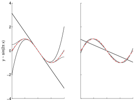
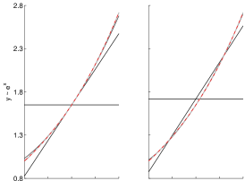
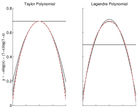
There is no simple computable remainder (corresponding to the one in Taylor series expansion) in Legendre polynomial approximation, but only bounds (see above). Therefore, we demonstrate the improvement in accuracy via an empirical approach using three representative transcendental functions: the sine function ($\sin(2\pi x)$), the exponential function ($\exp(x)$), and the entropy of a Bernoulli trial ($H(p)=-p\log p-(1-p)\log(1-p)$) in the interval $[0,1]$. Note that all three functions satisfy the boundedness condition $\left|{d^{n}y}/{dx^{n}}\right|\leq K\alpha^{n}$ above. For comparison, we approximate the functions with Taylor and Legendre polynomials using at most six non-zero coefficients (Figure 1). Because the sine function has odd symmetry about $x=1/2$ and the entropy function $H(p)$ is odd, the expansions of these function involve, respectively, polynomial degrees of 11 and 10 of even and odd order. We estimate the signal-to-noise ratio (SNR, in decibels) for approximations as

$$\mathrm{SNR}(f,\hat{f})=10\log_{10}\dfrac{\intop_{0}^{1}f^{2}}{\intop_{0}^{1}(f-\hat{f})^{2}}$$ (23)

to quantify the accuracy in approximation (Table 1).

(a) Entropy function

(b) Sine function

(c) Exponential function

Figure 1: Taylor and Legendre polynomial approximations at $x\in[0,1]$ Dashed red traces show the actual function evaluated for each $x$. Values of polynomial approximations are shown with solid traces, and successively darker colors indicate approximations using one (light-gray) to six (black) non–zero polynomial coefficients.

Table 1: Signal-to-noise ratios (in decibels) for the Taylor (T) and Legendre (L) polynomial approximations. Note the higher SNR for the Legendre polynomial approximation. The accuracy of Legendre polynomial approximation is significantly greater than that of Taylor approximation of equal order.

	$H(p)$		$\sin(2\pi x)$		$\exp(x)$
Order	T	L	T	L	T	L
1	11.12	11.20	-5.53	4.0	5.95	9.11
2	25.54	29.09	.96	20.56	20.76	29.78
3	42.64	50.60	14.23	44.32	27.74	41.13
4	61.84	74.64	32.18	73.10	32.29	42.04
5	82.73	100.64	53.76	105.73	35.67	55.12
6	105.06	128.22	78.31	141.49	38.36	60.05

Consistent with the theoretical considerations in above, these results show a rapid convergence of Legendre polynomials for increasing number of polynomial coefficients, and an improved accuracy compared to Taylor polynomials of the same order. Note that using six coefficients, even the least improvement (in the case of the exponential function) is 21.59 decibels (which amounts to an average error for the Legendre approximation 0.087 times the error for the Taylor approximation). The approximation for the sine function leads to an improvement of 63.18 decibels (that is, the error the Legendre approximation is 0.0007 times as that for the Taylor approximation on average). Note in Figure 1 that while the Taylor polynomial approximation has maximum accuracy at the midpoint, Legendre polynomial approximation distributes the error more uniformly throughout the entire interval. As a result, the squared error of is smaller and the SNR is larger in case of Legendre polynomials.

4 Conclusions

Our analytical and numerical results show that Legendre polynomials can substantially improve the speed and accuracy of function approximation compared to Taylor polynomials of the same order. The fast convergence of Legendre polynomials was noted in a prior study [4], but the geometric convergence in norm has not been shown analytically before. The geometric convergence rate is consistent with the general result of Srivastava [5] on the relation of the generalized rate of growth of an entire function to the rate of uniform convergence of a polynomial approximation on an arbitrary infinite compact set. And, it should be noted that the geometric convergence is not possible in general for $L_{p}$ approximants if $p\neq 2$ [6]. Thus, approximation using Legendre polynomials can provide significant performance improvements in practical applications. We also showed that Legendre polynomials has the additional advantage that an arbitrary function can be approximated using non-uniformly spaced points on a given interval. Importantly, its accuracy of approximation is substantially higher than that of the Taylor expansion with the same order of polynomials, with a uniform error distribution across the entire interval. Therefore, Legendre expansion, instead of Taylor expansion, should be used when global accuracy is important.

References

• [1] K. Weierstrass, Über die analytische darstellbarkeit sogenannter willkülicher functionen reeller argumente, Sitzungsberichte der Kniglich Preuischen Akademie der Wissenschaften zu Berlin 11 (1885) 633.
• [2] M. Abramowitz, I. Stegun, Handbook of mathematical functions, with formulas, graphs and Mathematical Tables, US Government Printing Office, 1964.
• [3] I. Gradshteyn, I. Ryzhik, R. Romer, Tables of integrals, series, and products, American Journal of Physics 56 (1988) 958.
• [4] Y.-M. Li, V. Y. Hsu, Curve offsetting based on legendre series, Computer Aided Geometric Design 15 (1998) 711.
• [5] G. S. Srivastava, S. Kumar, Uniform approximation of entire functions on compact sets and their generalized growth, New Zealand Journal of Mathematics 39 (2009) 33.
• [6] K. G. Ianov, S. E. B., Nongeometric convergence of best Lpsubscript𝐿𝑝L_{p} (p2)𝑝2(p\not=2) polynomial approximants, Proceedings of the American Mathematical Society 110 (1990) 377.