Improving free-energy estimates from unidirectional work measurements: theory and experiment

Abstract

We derive analytical expressions for the bias of the Jarzynski free-energy estimator from $N$ nonequilibrium work measurements, for a generic work distribution. To achieve this, we map the estimator onto the Random Energy Model in a suitable scaling limit parametrized by $(\log N)/\mu$, where $\mu$ measures the width of the lower tail of the work distribution, and then compute the finite-$N$ corrections to this limit with different approaches for different regimes of $(\log N)/\mu$. We show that these expressions describe accurately the bias for a wide class of work distributions, and exploit them to build an improved free-energy estimator from unidirectional work measurements. We apply the method to optical tweezers unfolding/refolding experiments on DNA hairpins of varying loop size and dissipation, displaying both near-Gaussian and non-Gaussian work distributions.

The accurate measurement of free-energy changes has important applications in physics, chemistry, and biology. Traditional measurement methods rely on reversible, near-equilibrium transformations, which however are often unfeasible. In recent years, new results in nonequilibrium statistical mechanics have suggested ways to measure free-energy changes from experiments (and simulations) far from equilibrium (see reviewJ for review). The Crooks fluctuation theorem (CFT) crooks states that the probability distribution $p(W)$ of the work $W$ done on a system driven out of equilibrium following an arbitrary finite-time protocol obeys the relation $p(W)/p_{R}(-W)=e^{(W-\Delta F)/k_{B}T}$. Here, $p_{R}(W)$ is the work distribution (WD) for the corresponding time-reversed protocol, $\Delta F$ is the free-energy difference between the final and initial equilibrium states JE , and $T$ is the temperature. Hence, $\Delta F$ can be estimated in bidirectional experiments by repeating many times the forward and reverse protocol, as demonstrated using single-molecule manipulation techniques bustamante ; collin . An asymptotically unbiased estimator based on the CFT is the acceptance ratio (AR) estimator shirts2004 .

In many experimental settings, which we shall call unidirectional, the reverse work cannot be measured. Examples are found in AFM pulling of biopolymers hummer-szabo ; kiang , steered simulations schulten , free-energy landscape reconstruction woodside , and single-molecule experiments on protein unbinding, intercalation, specific cation binding, antigen-antibody interactions, and non-native protein conformations. In these cases, an alternative method is provided by a corollary of the CFT, the Jarzynski equality (JE) $\langle e^{-W/k_{\tiny{\mbox{B}}}T}\rangle=e^{-\Delta F/k_{\tiny{\mbox{B}}}T}$, where $\langle\,\cdot\,\rangle$ is the expectation over $p(W)$ JE . Given $N$ work measurements $W_{1},\dots,W_{N}$ under the same protocol, the Jarzynski estimator

$$\Delta F_{N}=-\log{1\over N}\sum_{i=1}^{N}e^{-{W}_{i}}\,$$ (1)

converges to $\Delta F$ from above as $N\to\infty$ (here and henceforth we set $k_{\tiny{\mbox{B}}}T=1$ and express all work values in units of $k_{B}T$ at room temperature). In practice, convergence of $\Delta F_{N}$ requires that rare trajectories with $W_{i}<\Delta F$ be sufficiently represented, which in turn requires $N\gg\exp({D_{typ}})$, where $D_{typ}$ is the typical value of the dissipated work, $D=W-\Delta F$ jarzynski2006 . Therefore, $\Delta F_{N}$ is a reliable estimator of $\Delta F$ only when $D_{typ}$ is not much larger than $k_{\tiny{\mbox{B}}}T$. It is thus important to have a quantitative estimate of the bias $B_{N}=\Delta F_{N}-\Delta F$. The mathematical problem faced is that of calculating the distribution of a (log)sum of exponentials of i.i.d. random variables, Eq.(1), which depends on the system- and protocol-specific WD. No closed solution to this problem is available romeo , even for a Gaussian WD (GWD). Expansions in $N^{-1}$ ZW ; gore are only applicable when the bias is of order $N^{-1}$, i.e. smaller than the $O(N^{-\frac{1}{2}})$ statistical error and thus negligible. In the relevant regime $B_{N}\gg O(N^{-1})$, power-law interpolations in $N$ gore and other approximations romeo have been discussed, but no reliable analytical theory exists.

In this Letter, we derive analytical expressions for the bias expectation $\langle B_{N}\rangle$ for a wide class of WD’s and validate them by comparison with exact numerical simulations, also in the regime of large bias. We use these results to build an improved unidirectional free-energy estimator by correcting for the bias of Eq.(1). We then discuss unfolding/refolding experiments on DNA hairpins, which allow us to test our method against the bidirectional AR estimator.

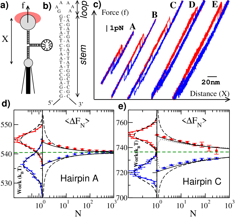
The experimental setup is shown in Fig. 1(a). We synthesized five hairpins (A,B,C,D,E) with identical stem and (GAAA…) loops of 4,6,12,16,20 bases, respectively [Fig.1b]. The hairpins are inserted between two short (29bp) dsDNA handles to improve signal-to-noise resolution ForLorManHayHugRit11 . The construct is tethered to two beads, one held by a pipette, the other by an optical trap created by counterpropagating laser beams Huguet10 . The light deflected by the trapped bead provides a direct measurement of the force acting on the molecule. By moving the trap away from the pipette at constant velocity, the hairpin is stretched until it unfolds. Subsequent reversal of the velocity causes the hairpin to refold. By repeating this cycle ($\approx 200-1000$ times per experiment) we collect the histogram of the WD’s $p_{U,R}(W)$ for the work to unfold (U) and refold (R) the hairpin, measured by integrating the force-distance curves (Fig.1c) for the forward and reverse part of each cycle (see Sec. 1 in Supp for details).

Figure 1: Bias measurements in DNA hairpins. a) Experimental setup. b) Hairpin B sequence. c) Examples of force-distance cycles for hairpins A-E. d) Left: histograms of $p_{U}(W)$ (upper), $p_{R}(-W)$ (lower) for hairpin A pulled at 400 nm/s. The horizontal line is the AR estimate $\Delta F_{AR}=540.5\,k_{B}T$, giving $|\langle D\rangle|=|\langle W\rangle-\Delta F_{AR}|$=4.3 $k_{\tiny{\mbox{B}}}T$ (U), 3.9 $k_{\tiny{\mbox{B}}}T$ (R). The lines are GWDs fitting the lower (upper) tail of $p_{U}(W)$ ($p_{R}(-W)$). Right: Jarzynski estimator $\langle\Delta F_{N}\rangle$ as a function of $N$ for U and R. Errors are estimated by jackknife. The lines represent $\Delta F_{AR}+\langle B_{N}\rangle$ with $\langle B_{N}\rangle$ given by Eq.(6) (dashed line) and Eq.(7) (continuous line) for the GWD case, assuming $D_{c}=\langle D\rangle=\mu$, where $\mu$ is estimated from the GWD fit to the tails. e) Same as d) but for hairpin C pulled at 65 nm/s [$|\langle D\rangle|$=13.6 $k_{\tiny{\mbox{B}}}T$ (U); 14.8 $k_{\tiny{\mbox{B}}}T$ (R)]. Also shown is $\Delta F_{AR}+\langle B_{N}\rangle$ with $\langle B_{N}\rangle$ given by Eq.(5) (dotted line).

We divide the data in blocks of $N$ cycles, compute $\Delta F_{N}$ for each block, and average over the blocks to estimate $\langle\Delta F_{N}\rangle$ for U and R separately. As shown in Fig.1(d,e) for hairpins A and C, $\langle\Delta F_{N}\rangle$ tends to the AR estimate $\Delta F_{AR}$ for large $N$, from opposite sides for U and R. Note that the dissipation increases with loop size and pulling speed.

We analyze theoretically the bias for a generic WD with finite mean and an unbounded lower tail which decays as

$$p(W)\sim q{\Omega^{\alpha-1}\over|W-W_{c}|^{\alpha}}\exp{\left(-\frac{|W-W_{c}|^{\delta}}{\Omega^{\delta}}\right)}\,,$$ (2)

for $W\ll W_{c}$, where $W_{c}$ is a characteristic work value, $\Omega>0$ measures the tail width and $q$ is a normalization constant. For the JE to hold, generally one must have $\delta>1$ tp . Two key parameters in the following are

$$\mu\equiv(\delta-1)\left({\Omega\over\delta}\right)^{\frac{\delta}{\delta-1}},\,\quad\lambda\equiv(\delta-1)\frac{\log N}{\mu}.$$ (3)

A saddle point calculation gives $\langle e^{-kD}\rangle\sim\exp{(\mu k^{\delta/(\delta-1)}-kD_{c})}$ for large $\Omega$, where $D_{c}=W_{c}-\Delta F$. Hence the JE implies $\mu\to D_{c}$ in this limit. An example of a WD obeying Eq.(2) is a GWD with mean $\langle W\rangle=W_{c}$ and variance $\sigma^{2}_{W}=\Omega^{2}/2$ (i.e. $\alpha=0$, $\delta=2$, $q=\pi^{-1/2}$), for which $\langle e^{-kD}\rangle=\exp({\mu k^{2}-k\langle D\rangle})$ and thus $\mu=\langle D\rangle=D_{c}=\sigma^{2}_{W}/2$ exactly for all $\Omega$. This relation allows one to define another unidirectional estimator $\Delta F_{v}=\langle W\rangle-\sigma^{2}_{W}/2$ wood , since $\Delta F_{v}=\Delta F$ for the GWD.

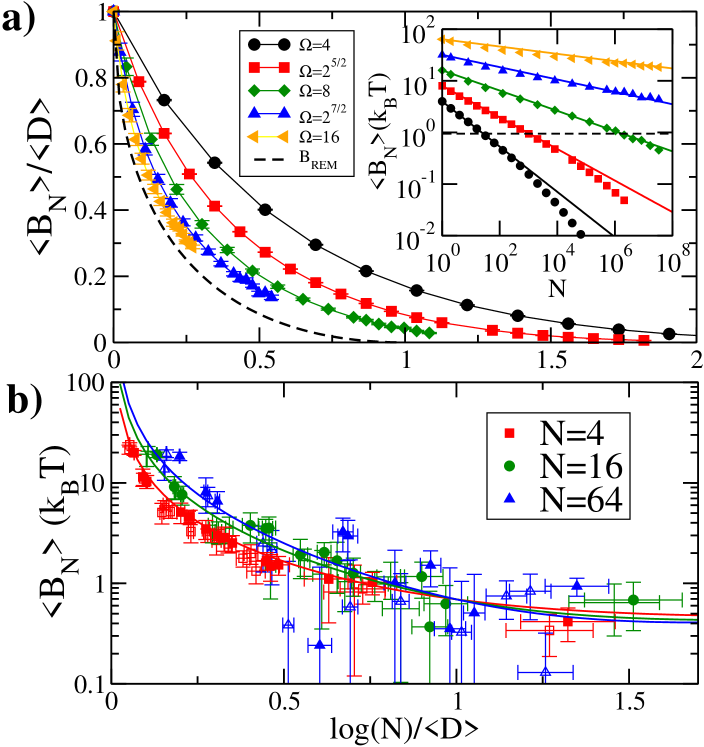
Scaling limit – Our strategy consists in computing first $\langle B_{N}\rangle$ in a suitable scaling limit, and then the finite-$N$ corrections to this limit. We obtain the scaling limit by mapping the problem onto the Random Energy Model (REM) derrida1 as $B_{N}=D_{c}+\log N-\log Z_{N}(\beta=\Omega/(\log_{2}N)^{(\delta-1)/\delta})$, where $Z_{N}(\beta)=\sum_{i=1}^{N}\exp[-\beta(\log_{2}N)^{(\delta-1)/\delta}E_{i}]$ is the REM partition function and the i.i.d. variables $E_{i}$ have a distribution decaying as $|E|^{-\alpha}\exp(-|E|^{\delta})$ for $E\ll-1$ derrida1 ; MB . From the known limit of $N^{-1}\langle\log Z_{N}(\beta)\rangle$ for $N\to\infty$ MB ; benarous we obtain $\langle B_{N}\rangle\to{\cal B}_{\mbox{\tiny{REM}}}$ in the scaling limit $(N,\Omega)\to\infty$ with $\lambda$ finite. For $\lambda>1$, all terms in $Z_{N}$ give a finite contribution and we find ${\cal B}_{\mbox{\tiny{REM}}}=D_{c}-\mu$. For $\lambda<1$, corresponding to the glass phase of the REM MB , $Z_{N}$ is dominated by a finite number of terms and we obtain

$${\cal B}_{\mbox{\tiny{REM}}}=D_{c}+\frac{\mu(\lambda-\delta\lambda^{1/\delta})}{\delta-1}=D_{c}+\log N-\Omega(\log N)^{1/\delta}\,.$$ (4)

Figure 2a shows the approach to the scaling limit as $\Omega$ increases, for the GWD case. Significant deviations occur for moderate $\Omega$, from which the need to compute finite-$N$ corrections is apparent.

Figure 2: Finite-$N$ corrections to the bias for a GWD. a) Convergence of $\langle B_{N}\rangle$ to its scaling limit. The points joined by lines are averages of $B_{N}=-\log N^{-1}\sum_{i}e^{-D_{i}}$ over many sets ($D_{1},\dots,D_{N}$) sampled from a GWD with variance $\Omega^{2}/2$ and mean $\langle D\rangle=\Omega^{2}/4$. The dashed line represents ${\cal B}_{\mbox{\tiny{REM}}}=\mu(1-\lambda^{1/2})^{2}$ [(Eq.(4) for $\delta=2$]. Inset of a): The unscaled data. The continuous lines represent Eq.(7). The horizontal dashed line $\langle B_{N}\rangle=1$ indicates the accuracy limit common in biophysical studies. b) Bias $|\langle B_{N}\rangle|$ (estimated as $|\langle\Delta F_{N}\rangle-\Delta F_{AR}|$) for all experiments on hairpins A,B,C and $N=4,16,64$, including both U and R. The pulling speed is in the range 25 - 300 nm/s and $|\langle D\rangle|$ is in the range 1 - 20 $k_{\tiny{\mbox{B}}}T$. The lines show Eq.(6) for the GWD.

Finite-$N$ corrections – One must distinguish three regimes, which require different analytical approaches: $\lambda>1$, $\lambda\ll 1$, and $\lambda\lesssim 1$. For $\lambda>1$, by partially resumming the $1/N$ expansion we obtain a closed expression for $\langle B_{N}\rangle$ that improves considerably over the truncated expansions previously considered ZW , which are valid only for $\lambda\gg 1$ (see Sec. 2.1 in Supp ). However, the most relevant regime in applications of the JE is $\lambda<1$, since in practice one usually has $N\ll\exp(D_{typ})$. In the limit $\lambda\ll 1$, using an extreme-value approach (Sec. 2.2 in Supp ) we obtain to leading order

$${\langle B_{N}\rangle}={\cal B}_{\mbox{\tiny{REM}}}-\lambda^{\frac{1-\delta}{\delta}}\left[\gamma_{E}+\frac{1-\alpha-\delta}{\delta}\log\log N+\log(q/\delta)\right]$$ (5)

where $\gamma_{E}$ is the Euler-Mascheroni constant. Cook and Derrida cook were able to compute the finite-$N$ corrections in the critical region $\lambda\lesssim 1$ for the GWD case in the context of the REM. We have extended their traveling-wave approach to the more general case of Eq.(2). In this way (see Sec. 2.3 in Supp for details) we recover Eq.(5) for $\lambda\ll 1$, while for $\lambda\lesssim 1$ we obtain

$${\langle B_{N}\rangle} = {\cal B}_{\mbox{\tiny{REM}}}+\gamma_{E}-\lambda^{\frac{1-\delta}{\delta}}\left[\gamma_{E}+\frac{1-\alpha-\frac{\delta}{2}}{\delta}\log\log N\right.$$ (6)

$$+ \left.{1\over 2}\log\frac{\pi q^{2}}{2\delta(\delta-1)}+\theta^{2}+\log\mbox{erfc}(\theta)\right]\,,$$

where erfc is the complementary error function and $\theta=(\lambda^{\frac{1-\delta}{\delta}}-1)\sqrt{\delta\log N}/\sqrt{2(\delta-1)}$.

Numerical test – Equations (5) and (6) provide, via Eqs.(3) and (4), explicit expressions for ${\langle B_{N}\rangle}$ as a function of $D_{c},\log N$, and the shape parameters $\delta,\Omega,\alpha,q$ of the WD tail. To illustrate the validity of these expressions, we computed numerically ${\langle B_{N}\rangle}$ by sampling $W_{i}$ from the GWD and from the Weibull WD (WWD): $p(W)=\delta\Omega^{-\delta}|W-W_{c}|^{\delta-1}\exp{-(|W-W_{c}|/\Omega)^{\delta}}$ for $W\leq W_{c}$; $p(W)=0$ for $W>W_{c}$, where $W_{c}$ is fixed numerically by imposing the JE. The WWD satisfies Eq.(2) ($\alpha=1-\delta$, $q=\delta$) and allows us to model tails falling faster ($\delta>2$) or more slowly ($\delta<2$) than a GWD. In this case $\langle W\rangle=W_{c}-\Omega\Gamma(1+\delta^{-1})$, $W_{typ}=W_{c}-\Omega\left(\frac{\delta-1}{\delta}\right)^{1/\delta}$.

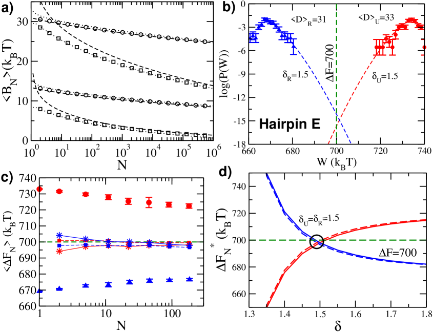
In their respective range of validity in $\lambda$, Eqs.(5) and (6) agree very well with the numerical data for the entire range tested ($1.1\leq\delta\leq 3$, $1.41\leq\Omega\leq 16$) also for large bias, as shown for some cases in Fig. 3(a) (for more examples see Fig.S4 in Supp ). Furthermore, substituting $D_{c}$ with $\mu$ in Eq.(4) worsens only slightly the agreement, an important observation for the following (see Sec. 2.5 in Supp ). In the special case of the GWD, Eq.(6) gives $\langle B_{N}\rangle=\log 2$ at $\lambda=1$. The empirical one-parameter power law

$${\langle B_{N}\rangle}=\langle D\rangle N^{-z},\quad z=-\langle D\rangle^{-1}\log\left(\log 2/\langle D\rangle\right),$$ (7)

interpolating between $\lambda=1$ and $\lambda=0$ (for which $\langle B_{N}\rangle=\langle D\rangle$) also fits fairly well the GWD data, as shown in Fig.2, although less so than Eq.(6) for large $\Omega$ (see also Fig.S4 in Supp ). A power-law fit of the bias in $N$ was proposed in Ref.gore . Figure 2(b) shows that the bias of all our experiments with mild dissipation is well described by Eq.(6) for a GWD.

Figure 3: free-energy recovery for non-Gaussian WDs. a) Analytical estimates of ${\langle B_{N}\rangle}$ as given in Eq.(5) (dashed lines) and Eq.(6) (dotted lines) with $D_{c}$ replaced by $\mu$, tested against simulated data for the WWD (symbols). From top to bottom, $(\delta,\Omega,\langle D\rangle)$= (1.1, 1.83, 31.0), (1.1, 1.68, 13.5), (1.5, 6, 30.1), (1.5, 4, 8.8). b) WD for hairpin E pulled at 130 nm/s and fitted WD tails assuming $\delta=1.5$ (dashed lines). The vertical line represents $\Delta F_{AR}$. c) $\langle\Delta F_{N}\rangle$ for U (circles) and R (triangles). Note the very slow convergence. The improved estimator $\Delta F^{*}_{N}$ obtained by correcting for the bias with Eq.(5) (squares) and Eq.(6) (stars) using $\delta=1.5$ converges quickly to a value consistent with $\Delta F_{AR}=700k_{B}T$ (dashed horizontal line) d) $\Delta F_{N}^{*}$ recovered from U and R as a function of $\delta$ for $N=182$. Using Eq.(5) (dashed lines) or Eq.(6) (continuous lines) gives nearly the same result.

Free-energy recovery method – The fact that Eqs.(5) and (6) describe well the bias when $D_{c}=\mu$ suggests an improved estimator $\Delta F^{*}_{N}$ applicable to any problem involving the logarithm of an exponential average: i) given $N$ measurements $W_{i}$, compute $\Delta F_{N}$ and the histogram of the WD; ii) estimate the shape parameters $\Omega,\delta,\alpha,q$ (and thus $\mu$) by fitting the histogram tail to Eq.(2), taking for instance the maximum of the WD for $W_{c}$ on_alpha ; iii) define $\Delta F^{*}_{N}=\Delta F_{N}-\langle B_{N}\rangle$ taking for $\langle B_{N}\rangle$ either Eq.(5) or (6) (depending on the value of $\lambda$) and setting $D_{c}=\mu$.

In the special case of the Jarzynski estimator, we must take into account the stronger constraint imposed by the CFT, which implies that $\langle e^{-W}\rangle$ is dominated by values of $W$ near the maximum $W^{\dagger}$ of the reverse WD Ritort04 . Sampling these very rare events is usually unfeasible, so there is no guarantee that the fit to the measured $p(W)$ will continue to hold near $W^{\dagger}$. Nevertheless, we argue that a distinction should be made between near-Gaussian and non-Gaussian tails. In the former case (i.e. when the tail can be fitted with $\delta\approx 2$), it is reasonable to assume that the fit will hold near $W^{\dagger}$, hence, $\Delta F^{*}_{N}$ should give a good estimate. The distance from a GWD can be self-consistently quantified a posteriori by the ratio $r=\sigma^{2}_{W}/(2\langle D\rangle)$ ($r=1$ for a GWD), taking $\langle D\rangle=\langle W\rangle-\Delta F^{*}_{N}$.

We return now to our DNA experiments, for which we can compare the unidirectional estimators $\Delta F_{N},\Delta F_{v},\Delta F^{*}_{N}$ separately for U and R with the bidirectional estimator $\Delta F_{AR}$. Figure 1(d) shows a case with mild dissipation, for which the bias of $\Delta F_{N}$ is small and all estimators converge. Figure 1(e) shows an experiment with intermediate dissipation. In this case sampling the tail of $p_{U}$ near the maximum of $p_{R}$ (or viceversa) would require an unfeasible number of cycles. Nevertheless, both tails are well fitted with $\delta=2,\alpha=0$. [They are not perfect GWD, being slightly asymmetric. Using $\langle D\rangle=\langle W\rangle-\Delta F_{AR}$ we obtain $r=$ 0.67 (U), 0.81 (R).] The curves in Fig.1(e) represent $\Delta F_{AR}+\langle B_{N}\rangle$ with $\langle B_{N}\rangle$ given by Eq.(5), (6), (7). We find that $\Delta F_{N}^{*}$ agrees with $\Delta F_{AR}$ within its statistical error for $N\geq 5$, for all three expressions. This represents a significant improvement over the variance estimator, which has a bias $\Delta F_{v}-\Delta F_{AR}=4.3\pm 0.8$ (U), $-2.9\pm 0.8$ (R), and over the uncorrected Jarzynski estimator. For instance, we have $\Delta F_{N}-\Delta F_{AR}=5.8\pm 3.0$ (U), $-6.6\pm 2.0$ (R) for $N=36$, and $\Delta F_{N}-\Delta F_{AR}=5.1\pm 0.6$ (R) for $N=289$. Furthermore, the fitted WD satisfy fairly well the CFT (see Sec. 4 in Supp ), giving further confidence in the consistency of the method.

Finally, we consider an experiment where the tails are far from a GWD and the dissipation is large (Fig.3). In this case the WDs are wide apart [Fig.3(b)] and $\langle\Delta F_{N}\rangle$ converges very slowly [(Fig.3(c)]. Equation (2) fits reasonably well the WD tails for a fairly broad range of $\delta$ values (we take $\alpha=0$ for simplicity on_alpha ). The estimator $\Delta F_{N}^{*}$ is shown in Fig.3d: the pronounced dependence on $\delta$ and the discrepancy between U and R confirm that the predictive power of Eqs.(5,6) relies on accurately knowing $\delta$ (see Sec. 3 in Supp for other examples). Note also that Eqs.(5,6) are ill-defined as the exponent $\delta$ approaches 1 tp . As $\delta$ decreases the fitted tails satisfy less and less the CFT (see Sec. 4 in Supp ), signaling that $\delta$ must increase further out in the tails. It is an open problem to generalize our analytical approach to an effective $\delta$ varying with $W$.

In summary, we obtained analytical expressions for the bias of the Jarzynski estimator, and showed that they can be used to obtain improved unidirectional estimates of the free energy of mechanical unfolding of DNA hairpins, provided the WD tail is described by a compressed exponential over a wide enough range of work values. These results are applicable to many unidirectional experiments and simulations, and are relevant to other contexts involving sums of random exponentials.

We thank N. Skantzos for discussions in the initial stages of this work. MP thanks NORDITA for hospitality. Work supported by MICINN (FIS2006-13321-C02-01, FIS2007-3454), HFSP Grant No. RGP55-2008, and ICREA Academia grants.

References

- (1) C. Jarzynski, Eur. Phys. J. B 64, 331 (2008).
- (2) G.E. Crooks, Phys. Rev. E 60, 2721 (1999).
- (3) C. Jarzynski, Phys. Rev. Lett. 78, 2690 (1997).
- (4) J. Liphardt et al., Science 296, 1832 (2002).
- (5) D. Collin et al., Nature 437, 198 (2005).
- (6) M. R. Shirts, E. Bair, G. Hooker and V. S. Pande, Phys. Rev. Lett. 91, 140601 (2003).
- (7) G. Hummer and A. Szabo, PNAS 98, 3658 (2001).
- (8) N. C. Harris and C.-H. Kiang, Phys. Rev. E 79, 041912 (2009).
- (9) M. O. Jensen, S. Park, E. Tajkhorshid and K. Schulten, PNAS 99 6731 (2002).
- (10) A.N. Gupta et al.,, Nat. Phys. (2011) doi:10.1038/nphys2022.
- (11) C. Jarzynski, Phys. Rev. E 73, 046105 (2006).
- (12) M. Romeo, V. Da Costa, and F. Bardou, Eur. Phys. J. B 32, 513 (2003).
- (13) D. M. Zuckerman and T. B. Woolf, Phys. Rev. Lett. 89, 180602 (2002); J. Stat. Phys. 114, 1303 (2004).
- (14) J. Gore, F. Ritort, and C. Bustamante, PNAS 100 12564 (2003).
- (15) Since is slowly varying compared to the exponential, in fitting Eq.(2) to experiments one can safely set .
- (16) N. Forns et al., Biophys. J. 100, 1765 (2011).
- (17) J. M. Huguet et al., PNAS 107, 15431 (2010).
-
(18)
See Supplemental Material at
http://link.aps.org/
supplemental/10.1103/PhysRevLett.107.060601 for the appendices. - (19) The JE can also be satisfied with . This marginal case requires a separate analysis.
- (20) R.H. Wood, W.F.C. Muhlbauer, and P.T. Thompson, J. Phys. Chem. 95, 6670 (1991).
- (21) B. Derrida, Phys. Rev. B 24, 2613 (1981).
- (22) J.-P. Bouchaud and M. Mézard, J. Phys. A 30 7997 (1997).
- (23) The scaling limit of the REM has been studied rigorously in G. Ben Arous, L.V. Bogachev, S.A. Molchanov, Prob. Th. Rel. Fields, 132, 579 (2005); A. Bovier, I. Kurkova, and M. Löwe, Ann. Probab., 30, 605 (2002).
- (24) J. Cook and B. Derrida, J. Stat. Phys. 63, 505 (1991).
- (25) F. Ritort, J. Stat. Mech. P10016 (2004).