Two-dimensional kinematics of SLACS lenses – IV. The complete VLT–VIMOS data set

Abstract

This paper presents the full VLT/VIMOS-IFU data set and related data products from an ESO Large Programme with the observational goal of obtaining two-dimensional kinematic data of early-type lens galaxies, out to one effective radius. The sample consists of 17 early-type galaxies (ETG) selected from the SLACS gravitational-lens survey. The galaxies cover the redshift range from 0.08 to 0.35 and have stellar velocity dispersions between 200 and 350 km/s. This programme is complemented by a similar observational programme on Keck, using long-slit spectroscopy. In combination with multi-band imaging data, the kinematic data provide stringent constraints on the inner mass profiles of ETGs beyond the local universe. Our Large Programme thus extends studies of nearby early-type galaxies (e.g. SAURON/ATLAS3D) by an order of magnitude in distance and toward higher masses. We provide an overview of our observational strategy, the data products (luminosity-weighted spectra and Hubble Space Telescope images) and derived products (i.e. two-dimensional fields of velocity dispersions and streaming motions) that have been used in a number of published and forthcoming lensing, kinematic and stellar-population studies. These studies also pave the way for future studies of early-type galaxies at $z\approx 1$ with the upcoming extremely large telescopes.

1 Introduction

The formation and evolution of early-type galaxies (ETGs) is a widely studied topic in present-day astrophysics, in particular due to a number of tight correlations between their observables, such as structural parameters, kinematics, colours and central supermassive black-hole masses (e.g. Illingworth, 1977; Sandage & Visvanathan, 1978; Djorgovski & Davis, 1987; Dressler et al., 1987; Ferrarese & Merritt, 2000; Gebhardt et al., 2000). See Renzini (2006) for a recent review. These correlations seem hard to explain at first sight in the hierarchical CDM formation paradigm (e.g. Binney, 1978; Blumenthal et al., 1984), where ETGs are seen as the end products of the stochastical merging of smaller building blocks (e.g. spiral galaxies; Toomre & Toomre, 1972; Barnes, 1992).

Both observational and theoretical studies have progressed rapidly over the last decade, largely thanks to major observational programmes conducted on the ground and from space (e.g. 2dF, SDSS, COSMOS, COMBO17; Colless et al., 2001; Bernardi et al., 2003; Scarlata et al., 2007; Faber et al., 2007) and due to the large-scale numerical simulations nowadays affordable by supercomputers (e.g. Hopkins et al., 2006). The SAURON and ATLAS^3D projects provide detailed analysis on substantial samples of nearby ETGs based on deep integral-field spectroscopic data and serve as a local benchmark for ETG studies (e.g. Cappellari et al., 2007; Emsellem et al., 2007; Emsellem et al., 2011).

Despite the tremendous increase in data volume and computational power, many questions remain very difficult to answer. This is due to several factors: (i) the types of available data (usually only luminosity-weighted kinematics and imaging) and their quality (in terms of signal-to-noise ratio and spatial/spectral resolution) have remained limited compared to their volume, (ii) mass modeling techniques often suffer from intrinsic degeneracies that are hard to overcome without very high quality data that can only be obtained for small samples of nearby ETGs. ETG studies that are now conducted beyond the local Universe with 8–10 m-class and space-based telescopes suffer from many of the same issues that similar studies of the local Universe, with 4 m-class telescopes, faced more than a decade ago.

One of the prevailing and, even today, still not precisely answered questions is how important dark matter is in the inner baryon-dominated regions of ETGs (e.g. Saglia et al., 1992; Saglia et al., 1993; Bertola et al., 1993; Bertin et al., 1994; Carollo et al., 1995; Gerhard et al., 1998; Loewenstein & White, 1999; Gerhard et al., 2001; Keeton, 2001; Romanowsky et al., 2003; Mamon & Łokas, 2005; de Lorenzi et al., 2009). Open questions include in particular the following: (i) How much dark matter is there precisely inside the inner few effective radii of ETGs and how is it distributed? (ii) How do the stellar and dark matter distributions of ETGs evolve with cosmic time and are there trends with galaxy mass? (iii) Do these observations agree with theoretical predictions?

Because dark matter is not directly observable but can only be inferred from other observations, these questions are particularly difficult to answer for more distant ETGs where data quality progressively deteriorates due to lack of signal-to-noise, even with the largest ground-based telescopes. To overcome a number of these hurdles, several systematic programmes were initiated over the last decade to combine the constraints of strong gravitational lensing with those of stellar kinematics (LSD and SLACS; e.g. Koopmans & Treu, 2002; Treu & Koopmans, 2004; Bolton et al., 2006; Treu et al., 2006; Koopmans et al., 2006; Koopmans et al., 2009; Bolton et al., 2008; Auger et al., 2009). This combination has turned out particularly powerful in breaking degeneracies in ETG mass models, despite the limited quality of the kinematic data (e.g. Treu & Koopmans, 2004; Koopmans et al., 2006; Koopmans et al., 2009; Auger et al., 2010). The reason is that the mass enclosed by the Einstein radius of a lens galaxy can be accurately determined and breaks the usual mass-anisotropy degeneracy of ETGs to a large extent (see e.g. Koopmans, 2004, for an explanation based on a simple power-law model).

Whereas the LSD and SLACS programmes used predominantly luminosity-weighted stellar velocity dispersions and were modeled using the spherical Jeans equation (e.g. Koopmans & Treu, 2003; Treu & Koopmans, 2004), one might argue that (slowly) rotating systems and/or systems with orbital anisotropy cannot be modeled properly that way (see for example the discussion in Kochanek, 2006). To address these valid issues, a new and substantially larger observational programme of a sub-sample of SLACS lenses, using observations with the VLT and Keck, was started in 2006 (Czoske et al., 2008; Czoske et al., 2009; Barnabè et al., 2010) to obtain two-dimensional kinematic fields (both first and second moments of the line-of-sight velocity distribution) out to their effective radii, complemented with a rigorous modeling effort based on two-integral axisymmetric models (Barnabè & Koopmans, 2007; Barnabè et al., 2009). The self-consistent combination of gravitational-lensing and stellar-kinematic data sets allows better constraints to be set on the mass distribution of ETGs (Czoske et al., 2008; Barnabè et al., 2009, 2010, 2011), but also to test less rigorous methods that might still have to be used at even higher redshifts (i.e. $z\ga 0.5$) until IFU observations from the next generation of telescopes (such as ESO’s ELT) become available.

Whereas the above-mentioned results show that these data provide more precise and accurate results on the total mass profile of ETGs in the inner few effective radii, several problems still remain that are critical for our understanding of galaxy formation. For example, what fraction of the mass inside several effective radii is due to dark matter and what are the relative mass distributions of the stellar and dark-matter components? This is much harder to answer with kinematic and lensing data alone, since there are many combinations of the stellar and dark-matter distributions that lead to similar lensing and kinematic data (Treu & Koopmans, 2004; Barnabè et al., 2009). If, on the other hand, the stellar mass-to-light ratio can be determined independently, these degeneracies can mostly be lifted. This assumes, however, that the broad-band colours provide sufficient information to break degeneracies in the IMF models, which in general they do not. Still, current constraints can already set limits on the IMF and stellar mass-to-light ratios that are becoming competitive (Grillo et al., 2008; Auger et al., 2009, 2010; Spiniello et al., 2011). To go beyond these broad-band inferred stellar mass-to-light ratios, one can also use the same (IFU) spectra to determine line indices from which more precise ages, metallicities and mass-to-light ratios of the ETG stellar population can be obtained (e.g. Trager et al., 2000). Whereas this information is going to be used in forthcoming publications, here we concentrate on describing the data for kinematic purposes.

In this paper, we present the full VLT/VIMOS-IFU data of our sample of 17 SLACS early-type lens galaxies, collected for these purposes. The sample is presented in Sect. 2. We describe the integral-field spectroscopic observations using VIMOS on the VLT in Sect. 3.1 and summarize the HST observations as needed for this project in Sect. 3.2. The data reduction of the IFU data is described in some detail in Sect. 4, and the kinematic analysis, i.e. the derivation of two-dimensional maps of line-of-sight velocity and velocity dispersion, in Sect. 5. In Sect. 6, we provide a list of additional objects that are visible in the VIMOS/IFU field of view around the lens galaxies. Finally, we conclude in Sect. 7. Appendix A gives a recipe for estimating the expected photon noise on the reduced spectra based on a simple model.

The fully self-consistent combined lensing/dynamics analysis of the data described in this paper is presented in the companion paper by Barnabè et al. (2011).

2 Sample

The sample described in this paper consists of seventeen early-type galaxies from the Sloan Digital Sky Survey that have been confirmed as secure gravitational-lens systems in the SLACS survey.

The SLACS survey searches for gravitational lens systems in the spectroscopic data of a subsample of SDSS galaxies comprising the luminous red galaxy sample (Eisenstein et al., 2001) and passive members of the MAIN sample (Strauss et al., 2002), defined as having rest-frame H $\alpha$ equivalent widths less than $1.5$ Å. The presence of emission lines at a redshift higher than that of the target galaxy in the SDSS spectra indicates that there is a background galaxy within the fibre, which may have been lensed. Candidates were selected for follow-up snapshot imaging with HST, allowing in most cases a robust confirmation or rejection of the lensing hypothesis. See Bolton et al. (2006) for details on the selection procedure. Treu et al. (2006) conducted a number of tests to verify that the SLACS lens sample is statistically indistinguishable from the parent samples. Results on the structure of the early-type lens galaxies can therefore be taken as representative for the population of (massive) early-type galaxies as a whole.

In order to be observable from Paranal, lens systems close to the equator ($\delta<15\degr$) were selected from the (mostly northern) SLACS catalogue. The final sample of 17 systems chosen for VIMOS/IFU follow-up is evenly distributed in right ascension.

The location of the 84 early-type SLACS galaxies studied by Auger et al. (2009) in the parameter space of redshift and velocity dispersion is shown in Fig. 1. The seventeen galaxies from the VIMOS/IFU subsample are marked; they are representative of the full SLACS early-type galaxy sample. Fig. 1 also shows the 48 local early-type galaxies studied by the SAURON team (Emsellem et al., 2004), as well as 17 early-type galaxies in the Coma cluster studied by Thomas et al. (2007). The VIMOS/IFU sample represents a major step out to cosmological distances compared to the SAURON and Coma samples. In terms of velocity dispersion, it overlaps with the more massive half of the SAURON sample and thus lends itself to comparison of the structure of early-type galaxies at $z\ga 0.1$ to their local counterparts.

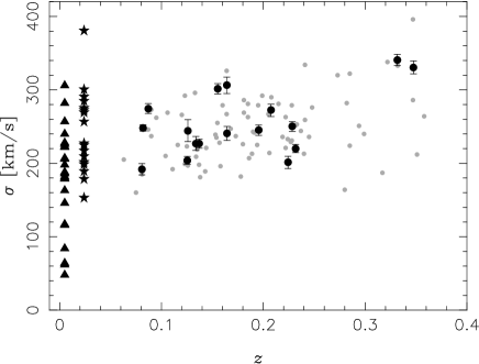
Figure 1: Distribution of the SLACS/IFU sample in redshift and velocity dispersion. The velocity dispersion measurements are taken from this paper, the error bars are statistical errors. For comparison, the SLACS early-type sample of Auger et al. (2009, grey points), the SAURON sample at redshift $z\approx 0$ (triangles: Emsellem et al., 2004) and a sample of Coma cluster early-type galaxies (stars: Mehlert et al., 2000; Corsini et al., 2008) are shown.

Table 1: The VIMOS/IFU sample. Apparent brightness $m_{V}$, effective radius $R_{\mathrm{eff},V}$ and Einstein radius $\theta_{\mathrm{Einst}}$ are from Auger et al. (2009). Redshifts and SDSS velocity dispersion are from Bolton et al. (2008). VIMOS velocity dispersions were measured from aperture-integrated spectra from the IFU data; errors include only the effect of noise, not of template mismatch (5–10 %, Sect. 5.1). The last two columns specify the grism used for each object and the number of observing blocks spent on each target.

Galaxy	$\alpha_{\mathrm{J2000}}$	$\delta_{\mathrm{J2000}}$	$m_{V}$	$R_{\mathrm{eff},V}$	$\theta_{\mathrm{Einst}}$	$z_{\mathrm{lens}}$	$z_{\mathrm{source}}$	$\sigma_{\mathrm{SDSS,B08}}$		$\sigma_{\mathrm{VIMOS}}$	Grism	OBs
				(arcsec)	(arcsec)			($\mathrm{km\,s^{-1}}$)		($\mathrm{km\,s^{-1}}$)
SDSS J0037	$00$:$37$:$53.21$	$-09$:$42$:$20.1$	$16.90$	$2.68$	$1.53$	$0.1955$	$0.6322$	$279$$\pm$	$10$	$245.3^{+6.9}_{-7.2}$	HR_Blue	9
SDSS J0216	$02$:$16$:$52.54$	$-08$:$13$:$45.3$	$18.36$	$2.97$	$1.16$	$0.3317$	$0.5235$	$333$$\pm$	$23$	$340.7^{+7.8}_{-7.7}$	HR_Orange	14
SDSS J0912	$09$:$12$:$05.31$	$+00$:$29$:$01.2$	$16.56$	$4.29$	$1.63$	$0.1642$	$0.3239$	$326$$\pm$	$12$	$306.5^{+10.9}_{-11.4}$	HR_Blue	4
SDSS J0935	$09$:$35$:$43.93$	$-00$:$03$:$34.8$	$17.71$	$4.12$	$0.87$	$0.3475$	$0.4670$	$396$$\pm$	$35$	$330.4^{+9.0}_{-8.5}$	HR_Orange	12
SDSS J0959	$09$:$59$:$44.07$	$+04$:$10$:$17.0$	$17.94$	$1.51$	$0.99$	$0.1260$	$0.5350$	$197$$\pm$	$13$	$244.2^{+15.2}_{-14.7}$	HR_Orange	4
SDSS J1204	$12$:$04$:$44.07$	$+03$:$58$:$06.4$	$17.45$	$1.65$	$1.31$	$0.1644$	$0.6307$	$267$$\pm$	$17$	$240.8^{+9.3}_{-9.5}$	HR_Orange	5
SDSS J1250A	$12$:$50$:$28.26$	$+05$:$23$:$49.1$	$17.77$	$1.91$	$1.13$	$0.2318$	$0.7953$	$252$$\pm$	$14$	$219.9^{+5.7}_{-5.4}$	HR_Orange	6
SDSS J1250B	$12$:$50$:$50.52$	$-01$:$35$:$31.7$	$15.68$	$4.01$	–	$0.0871$	$0.3529$	$246$$\pm$	$9$	$274.4^{+6.9}_{-6.7}$	HR_Orange	6
SDSS J1251	$12$:$51$:$35.71$	$-02$:$08$:$05.2$	$17.71$	$5.34$	$0.84$	$0.2243$	$0.7843$	$233$$\pm$	$23$	$201.5^{+8.1}_{-8.7}$	HR_Orange	12
SDSS J1330	$13$:$30$:$45.53$	$-01$:$48$:$41.6$	$17.56$	$1.36$	$0.87$	$0.0808$	$0.7115$	$185$$\pm$	$9$	$191.8^{+7.8}_{-7.5}$	HR_Orange	3
SDSS J1443	$14$:$43$:$19.62$	$+03$:$04$:$08.2$	$17.62$	$1.38$	$0.81$	$0.1338$	$0.4187$	$209$$\pm$	$11$	$226.8^{+9.7}_{-9.2}$	HR_Orange	4
SDSS J1451	$14$:$51$:$28.19$	$-02$:$39$:$36.4$	$16.92$	$2.64$	$1.04$	$0.1254$	$0.5203$	$223$$\pm$	$14$	$203.9^{+5.4}_{-5.3}$	HR_Orange	7
SDSS J1627	$16$:$27$:$46.45$	$-00$:$53$:$57.6$	$17.87$	$2.05$	$1.23$	$0.2076$	$0.5241$	$290$$\pm$	$14$	$272.6^{+7.8}_{-8.9}$	HR_Orange	11
SDSS J2238	$22$:$38$:$40.20$	$-07$:$54$:$56.0$	$17.18$	$2.41$	$1.27$	$0.1371$	$0.7126$	$198$$\pm$	$11$	$226.8^{+6.2}_{-6.2}$	HR_Orange	6
SDSS J2300	$23$:$00$:$53.15$	$+00$:$22$:$38.0$	$18.19$	$1.93$	$1.24$	$0.2285$	$0.4635$	$279$$\pm$	$17$	$250.4^{+6.4}_{-7.0}$	HR_Orange	10
SDSS J2303	$23$:$03$:$21.72$	$+14$:$22$:$17.9$	$16.77$	$3.54$	$1.62$	$0.1553$	$0.5170$	$255$$\pm$	$16$	$301.5^{+7.1}_{-7.1}$	HR_Orange	11
SDSS J2321	$23$:$21$:$20.93$	$-09$:$39$:$10.3$	$15.27$	$4.79$	$1.60$	$0.0819$	$0.5324$	$249$$\pm$	$8$	$248.1^{+4.4}_{-4.4}$	HR_Blue	5

3 Observations

3.1 Integral-field spectroscopy

We have obtained integral-field spectroscopic observations of 17 systems using the integral-field unit (IFU) of VIMOS (Le Fèvre et al., 2001).

VIMOS is a wide-field imager, multi-object and integral-field spectrograph mounted at the Nasmyth focus B of the Very Large Telescope UT3 (Melipal) on Paranal, Chile. The integral-field unit samples the focal plane with a total of 6400 lenslets, each of which is coupled to an optical fibre. The opposite ends of the fibres are arranged to form pseudo-slits of 400 fibres each. The light emerging from the pseudo-slit is dispersed in the usual way using grisms and optionally order-separating filters, and the resulting spectra are recorded on four $2\mathrm{k}\times 4\mathrm{k}$ EEV CCD chips. In low-resolution mode, the spectra from four pseudo-slits are stacked in the dispersion direction on each of the four CCDs. The arrangement is such that each CCD records the spectra from one quadrant of the field of the IFU head. In high-resolution mode, only the spectra from one pseudo-slit fit onto a CCD and only the central 1600 elements of the IFU head are used. The spatial scale in the focal plane can be chosen to be $0.67\,\mathrm{arcsec}$ or $0.33\,\mathrm{arcsec}$ per spectral element. We used the large spatial scale and high-resolution mode and thus work with a field of view of $27\arcsec\times 27\arcsec$ covered by $40\times 40$ spectra.

Three of the 17 systems of the sample were observed as ESO Programme 075.B-0226 (henceforth the “pilot programme”) between June 2005 and January 2006. The remaining fourteen systems were the targets of an ESO Large Programme, 177.B-0682 (the “main programme”), and were observed between April 2006 and March 2007. For the pilot programme, the high-resolution blue grism (HR-Blue) was used, which has a nominal resolution of $R=2550$ and covers the wavelength range $4000\,$Å to 6200 Å; for the main programme the HR-Orange grism was used, which covers a somewhat redder wavelength range between 5000 Å and 7000 Å at comparable resolution ($R=2650$).

All observations were carried out in service mode. For this, the total observing time was broken down in observing blocks (OBs), each with an execution time of one hour and comprising science and calibration exposures. For the pilot programme, three dithered science exposures of integration time 555 seconds on one target were taken during an OB. For the main programme, a single exposure per OB was taken, with integration time 2060 seconds. The main observational constraint for scheduling the OBs for this project was a maximum seeing of $0.8\,\mathrm{arcsec}$ FWHM (full width at half maximum).

We followed ESO’s standard calibration plan which comprises three flat-field exposures and one arc-lamp exposure per OB, taken immediately after the science exposures. Bias exposures were taken during day time in blocks of five exposures.

Standard stars are observed at varying intervals by ESO staff and were therefore in most cases not available for the same nights that our science data were taken. They are useful for relative flux calibration but not for absolute spectro-photometric calibration.

3.2 HST imaging

Modelling stellar dynamics and the lens effect requires photometric information on both the lens galaxy and the lensed background source. We use various HST observations obtained for the SLACS project (see Bolton et al., 2008; Auger et al., 2009).

Lens modelling aims at reconstructing the two-dimensional surface-brightness distribution of the background source. This is obtained from high-resolution ACS images from which elliptical B-spline models of the lens galaxies were subtracted (see Bolton et al., 2008, for details). For eight systems, we have deep F814W images from Programmes 10494 and 10798 (Cycle 14, PI: L. Koopmans) consisting of four exposures. For the remaining systems only single exposure images from snapshot Programme 10174 (Cycles 13, PI: L. Koopmans) are available. The pixel scale of these images is $0.05\,\mathrm{arcsec}$.

The surface-brightness distributions of the lens galaxies are obtained from NICMOS F160W images from Programmes 10494, 10798 and 11202 (Cycle 16, PI: Koopmans). The full resolution images have a pixel scale of $0.05\,\mathrm{arcsec}$ and include four exposures for a total exposure time of $2560\,\mathrm{s}$. In order to have proper flux weights for the kinematic maps we resample the NICMOS images to the VIMOS/IFU grid with $0.67\,\mathrm{arcsec}$ per spatial pixel after convolution to match the point spread function (PSF) of the VIMOS data, taken to be Gaussian with FWHM of $0.8\,\mathrm{arcsec}$.

Three systems (J1251, J1627 and J2321) were not observed with NICMOS. For these systems we use the B-spline models to the F814W ACS images to estimate the surface brightness of the lens galaxy. We add random noise according to the ACS weight maps to mimic observational data.

All images were astrometrically registered using the measured position of the lens galaxy and in some cases additional objects visible in the VIMOS field of view.

The F814W images of the systems in the sample are shown in Fig. 2.

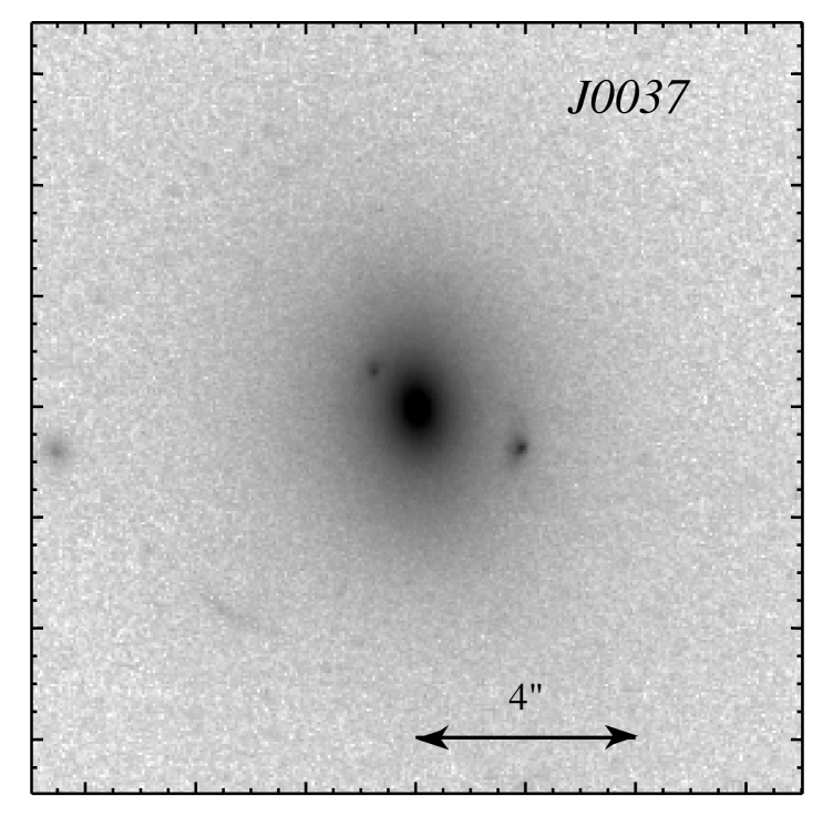
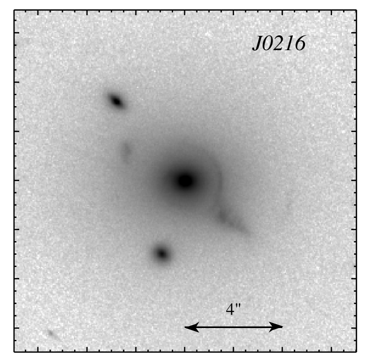
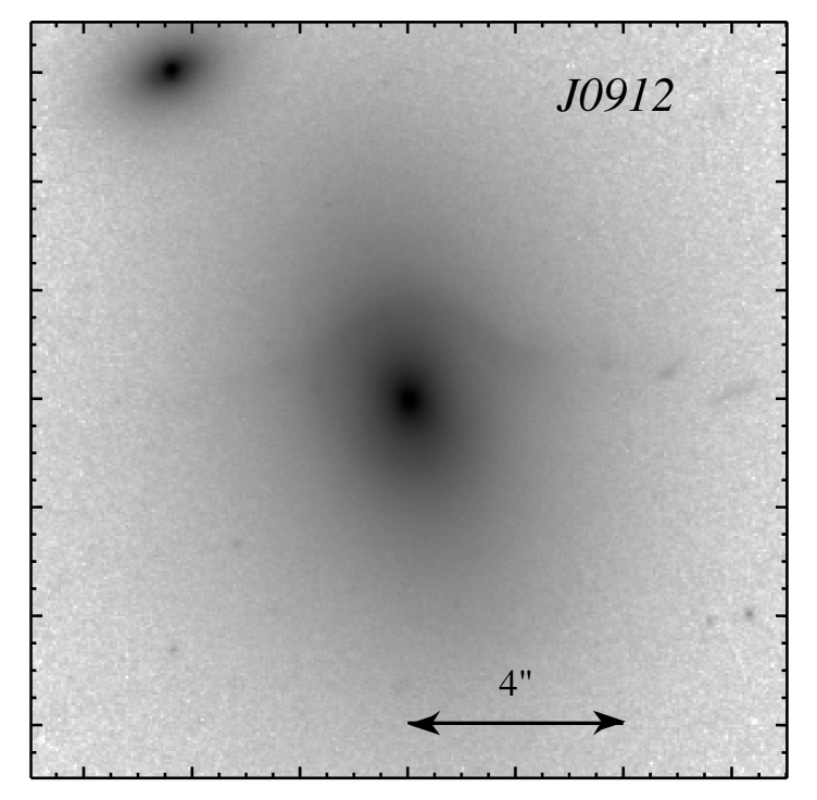
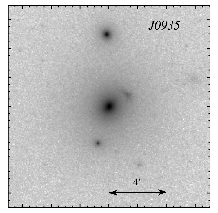
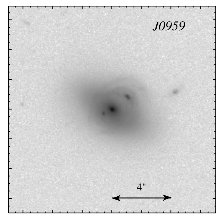
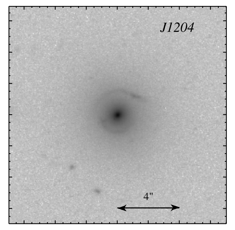
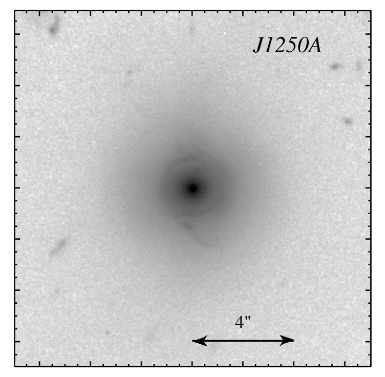
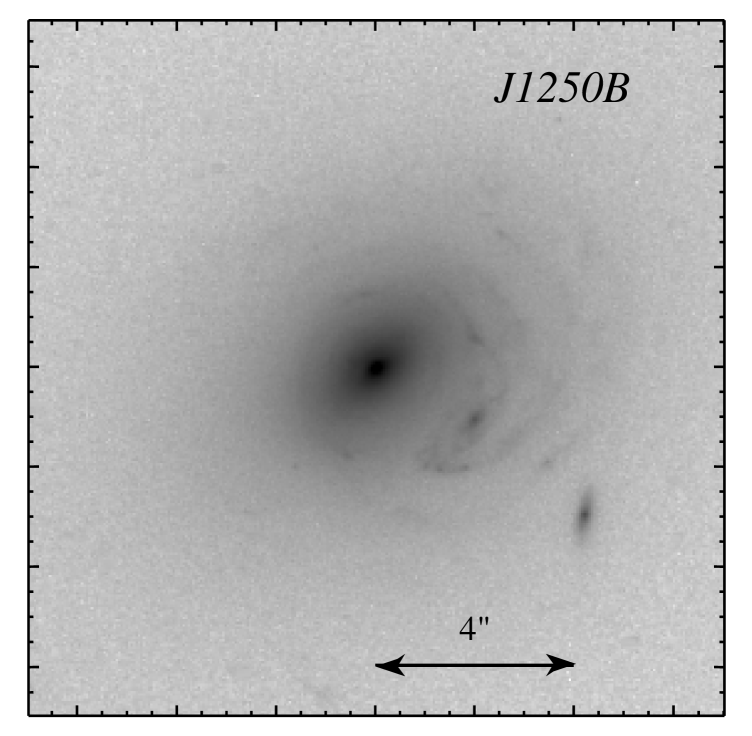
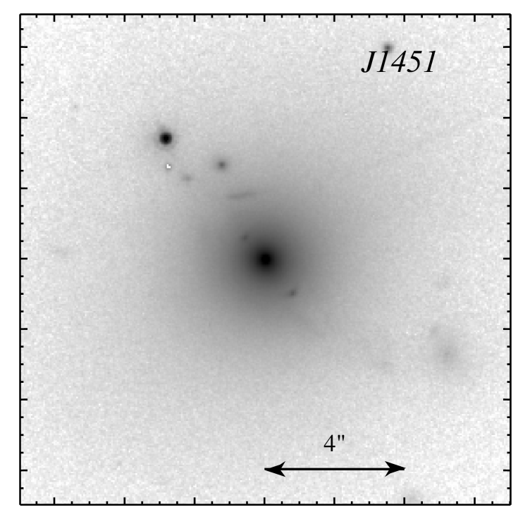
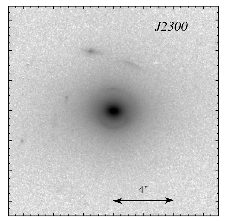
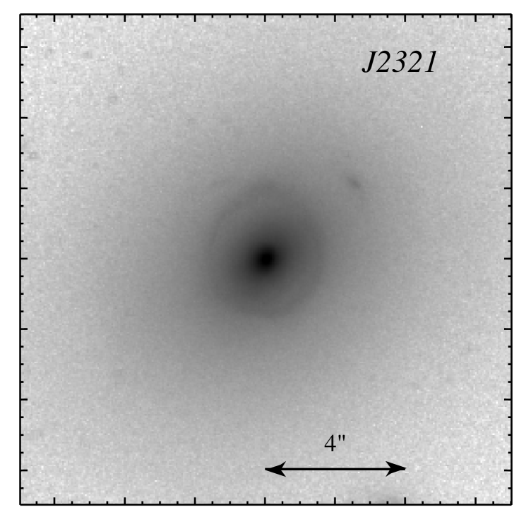
Figure 2: HST/F814W images of the systems in the sample. In images obtained in a snapshot programme cosmic ray hits were interpolated over for display purposes.

4 Data reduction

The VLT VIMOS/IFU data were reduced using the vipgi package which was developed within the framework of the VIRMOS consortium and the VVDS project. vipgi has been described in detail by Scodeggio et al. (2005) and Zanichelli et al. (2005). In Czoske et al. (2008), we have already given an overview of the data reduction procedure as applied to our data set, so that we restrict ourselves here to giving the main parameters.

The wavelength calibration is based on about 20 helium and neon lines spread over the wavelength range. Fitting a third-order polynomial results in residuals with root-mean-square of $\sim 0.075\,$Å, corresponding to $\sim 5\,\mathrm{km\,s^{-1}}$, significantly smaller than the spectral resolution and negligible in our analysis.

After rectification of the two-dimensional spectra onto a linear wavelength grid with a dispersion of $0.644$ Å per pixel, one-dimensional spectra are extracted for each fiber in an optimal way using the algorithm of Horne (1986). We refer to the resulting collection of one-dimensional spectra as a “data cube” even though the data structure is, strictly speaking, not a three-dimensional cube. Spectra are labeled by the spatial coordinates $L$ and $M$ (or world coordinates $\alpha$ and $\delta$).

A relative flux calibration (giving correct flux as a function of wavelength) is done using the standard observation nearest in time to the execution of a given science observing block. Since this does not necessarily come from the same night as the science exposures and no attempt is made to observe them at the same airmass, the standard observations can only provide a relative correction but no absolute spectro-photometric calibration.

The varying transmissivity of the fibres is corrected by measuring and comparing the flux under a sky line in the different extracted spectra. We used [O i] $\lambda 5577.4$ for this purpose, integrating over a range of seven pixels ($4.2~{}$Å) and subtracting an estimate of the underlying continuum from a window of five pixels on one side of the line.

The observed galaxies are smaller than the field of view of VIMOS/IFU, leaving a sufficient number of fibres pointing at blank sky to permit good sky subtraction. These sky fibres are identified automatically from a histogram of the total fluxes recorded in each fibre, integrated over the entire wavelength range. The sky fibres are then grouped according to the shape of the [O i] $\lambda 5577$ line, a mean over the sky spectra in each group is computed and subtracted from each row according to the group it is judged to belong to. The sky subtraction works well even redwards of 6200 Å, where the sky is dominated by the OH molecular bands.

The data cubes from all the exposures on a field are finally combined into a final data cube by taking the median. Telescope offsets between the exposures are corrected through spatial shifting by an integer number of fibres. Subpixel shifts could in principle be corrected for by interpolation between adjacent fibres but in practice it turns out that the centroids of the galaxies in image reconstructions of the individual exposures are hard to measure to subpixel accuracy, given the level of accuracy of the fibre transmission correction and the resulting noise in the image reconstructions.

A short-coming of vipgi is that it does not provide noise estimates on the reduced spectra. Since proper weighting is desirable for the determination of kinematic and stellar population parameters, we reconstruct noise spectra from a simple model including photon noise and read-out noise. We require noise spectra for each spectral element in the data cube and for the aperture-summed spectra. It turns out that at each step of the reduction procedure, the noise estimate can be written as a rescaled version of the current intermediate data product, including the sky background. The necessary noise spectra can thus easily be produced by creating and rescaling a second data set, reduced in the normal manner but with sky subtraction turned off. A detailed derivation of the noise estimation procedure is given in Appendix A, which can also be read as a walk-through of the data reduction process.

Fig. 3 shows integrated spectra obtained by summing the one-dimensional spectra from fibres within elliptical apertures following the shape and size of each lens galaxy. Typical diameters of these apertures are around $4$ arcsec, i.e. a little larger than the 3 arcsec circular aperture used by the SDSS.

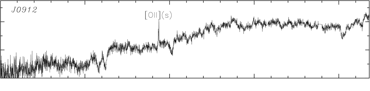
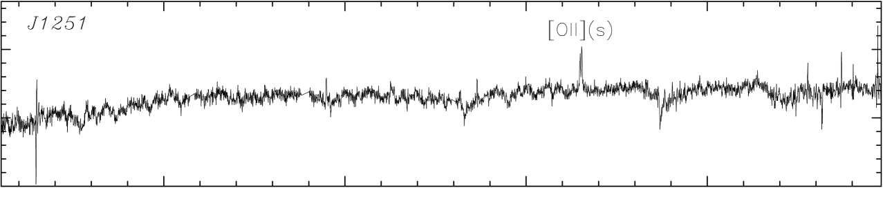
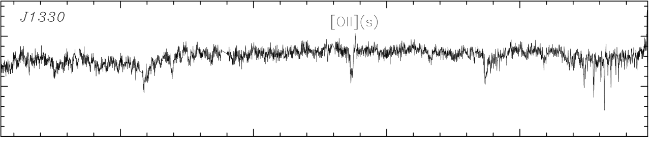
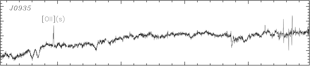
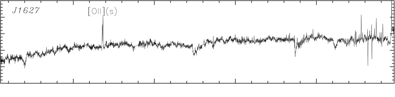
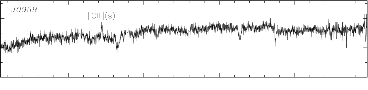
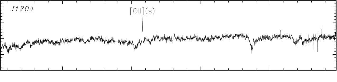
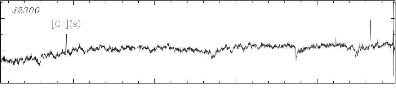
Figure 3: Global spectra obtained by adding spectra within elliptical apertures with diameters between 5 and 14 spaxels, matched to the surface brightness of the objects. Wavelengths are in Å. The three spectra top left are from the pilot programme and cover a different wavelength range then the spectra from the large programme. Emission lines from the sources are marked. The narrow residuals of sky lines at 5577 Å, 5890 Å and 6300 Å have been interpolated over for display purposes.

The spectra are typical for early-type galaxies, with strong metal absorption lines, in particular Ca i H and K, the G and the Mg b bands. With the exception of J2321 (Czoske et al., 2008), no significant emission lines from the lens galaxies are detected. This is true even for those galaxies that show clear disk and spiral structure in the HST images.

Most of the spectra clearly show [O ii] $\lambda 3727$ emission from the lensed source, although in some cases this line falls outside the wavelength range of the VIMOS spectra. In some cases, in particular J1250B and J1451, several Balmer emission lines from the source can be seen. These become more prominent in the residuals of the kinematic fits, described in Sect. 5.

5 Kinematic analysis

5.1 Method

Table 2: Stellar templates used for kinematic analysis of the VIMOS/IFU sample

Galaxy	Template star	Spectral type
J 0037	HD 249	K1 IV
J 0216	HD 195506	K2 III
J 0912	HD 121146	K3 IV
J 0935	HD 195506	K2 III
J 0959	HD 102328	K3 III
J 1204	HD 221148	K3 III
J 1250A	HD 145328	K1 III
J 1250B	HD 216640	K1 III
J 1251	HD 145328	K1 III
J 1330	HD 25975	K1 III
J 1443	HD 85503	K2 III
J 1451	HD 114092	K4 III
J 1627	HD 195506	K2 III
J 2238	HD 195506	K2 III
J 2300	HD 195506	K2 III
J 2303	HD 121146	K3 IV
J 2321	HD 77818	K1 IV

Many methods to determine the line-of-sight velocity distribution (LOSVD) of early-type galaxies from spectra have been proposed in the past (e.g. Rix & White, 1992; van der Marel & Franx, 1993; Cappellari & Emsellem, 2004). We use the conceptually simplest method, template-fitting in pixel space. Our method is implemented as a package (slacR) in the statistical language R (R Development Core Team, 2007), following descriptions from several authors, in particular van der Marel & Franx (1993) and Kelson et al. (2000). Compared to the version used in Czoske et al. (2008), we have modified and extended our method sufficiently to warrant a full description of the method here.

The model parameters $\mn@boldsymbol{\theta}$ are determined by minimizing the merit function

$$S=\sum_{i}\frac{1}{\sigma_{i}^{2}}\left(s_{i}-\hat{s}(\lambda_{i},{\mn@boldsymbol{\theta}})\right)^{2}\,,$$ (1)

where the sum extends over all “good” pixels $\lambda_{i}$ in the observed spectrum $s_{i}$. The observed spectrum is transformed to the rest frame of the respective lens galaxy prior to the analysis by dividing observed wavelengths by a factor $1+z_{\mathrm{lens}}$. The effective resolution of the spectrum is increased to $R(1+z_{\mathrm{lens}})$ compared to the nominal resolution $R$ of the spectrograph (Sect. 3.1).

The data-model $\hat{s}$ (in vector-matrix notation) is given by the equation

$$\hat{s}_{i}=[\mn@boldsymbol{G}*\mn@boldsymbol{t}](\lambda_{i})\,p^{(m)}(\lambda_{i})+q^{(n)}(\lambda_{i})+\epsilon_{i}\,.$$ (2)

Here, the vector $\mn@boldsymbol{G}$ is the LOSVD, taken to be a Gaussian in velocity, with kinematic parameters $v$ (streaming motion) and $\sigma_{v}$ (velocity dispersion). The vector $\mn@boldsymbol{t}$ is a stellar template spectrum, taken from the Indo-US library of stellar spectra (Valdes et al., 2004). Templates were chosen by fitting a random sample of IndoUS spectra to the aperture-integrated VIMOS/IFU spectra and selecting one of the best-fitting (in the least-squares sense) template candidates. We did not always choose the template giving the absolute minimum $\chi^{2}$: It was noticed that HD 195506 appeared among the best-fitting templates for several systems and was therefore chosen for all of these. Table 2 lists the templates used for the kinematic fits, as well as their spectral type and luminosity class. As expected, the selected template stars are predominantly late-type giants. The same template was used for fitting all the individual fibre spectra for each system. The effect of template mismatch on the derived kinematic parameters will be discussed below.

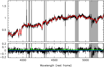
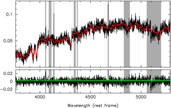
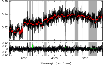
Figure 4: Kinematic fitting of spectra of system J0935. Top: global spectrum summed in an aperture of radius 2.3 arcsec, $S/N\approx 45$ per wavelength bin. Centre: single spaxel with $S/N\approx 23$ per bin. Bottom: single spaxel with $S/N\approx 12$ per bin. The top panel of each pair shows the spectrum and the template fit in red. The bottom panel shows the residuals with the expected noise level in green (Appendix A). The grey areas mark regions that were excluded from the fits. Wavelengths are given in the rest frame of the lens ($z=0.3475$). The [O ii] line from the source can be seen at 4057 Å in this plots.

For the kinematic fit, the template is first brought to the effective instrumental resolution of the observed spectrum by convolving with a kernel that is a Gaussian in wavelength. The convolution with the LOSVD $\mn@boldsymbol{G}$ is performed in $\log\lambda$ (equivalently: velocity), and the result is then resampled to the same wavelength grid as the data $\mn@boldsymbol{s}$, thus avoiding having to resample the data beyond what has been done during the data reduction. The functions $p^{(m)}(\lambda)$ and $q^{(n)}(\lambda)$ are multiplicative and additive correction polynomials of order $m$ and $n$, respectively. These polynomials are needed to correct any low-frequency differences between the galaxy and template spectra due to insufficient flux calibration, contamination by the continuum of the lensed background galaxy and other effects which are not related to the kinematics of the lens galaxy. In contrast to Czoske et al. (2008), where only a short wavelength range around a single spectral feature was used and a linear correction function was sufficient, we here use the full wavelength range. The coefficients are determined by a linear fit nested within the non-linear optimization for the kinematic parameters $v$ and $\sigma_{v}$. The orders of the polynomials are determined by inspecting large-scale systematics in the residuals from the fits; we obtain satisfactory corrections for $m=4$ and $n=6$.

A number of features in the spectra were excluded in the kinematic fits. Possibly present Balmer lines in the lens spectrum are due to younger stellar populations that are not adequately described by the late-type template stars. The strength of the Mg b band and Na D lines is enhanced compared to that in the galactic stars used as templates (Barth et al., 2002). Also masked were night-sky emission lines and atmospheric absorption features, as well as emission lines from the lensed background sources. Finally, a 3-$\sigma$ clipping algorithm (three iterations) was applied to detect possible outliers.

The noise $\mn@boldsymbol{\epsilon}$ is assumed to be normally distributed with mean zero and wavelength-dependent dispersion $\mn@boldsymbol{\sigma}_{\epsilon}$. Since vipgi does not produce noise estimates that take the details of the reduction procedure into account, we have to estimate the noise spectra after the fact, using a model including readout noise and photon noise as described in Sect. 4 and Appendix A. The average signal-to-noise ratio used to characterize a spectrum was determined by dividing the spectrum by its noise spectrum and taking the median. Signal-to-noise ratios are thus given per wavelength pixel of width 0.644 Å.

The noise was propagated to error estimates on the kinematic parameters using a Monte-Carlo method. Gaussian noise was added to the best-fit model with wavelength-dependent dispersion given by the corresponding noise spectrum and the resulting spectrum was fitted in the same way as the original spectrum. The quoted errors on the parameters of the original spectrum are the 16% and 84% percentiles of the kinematic parameters $v$ and $\sigma_{v}$ obtained from 300 such realizations.

The errors due to template mismatch can be estimated from the distribution of best-fit values determined with 755 stellar spectra of widely varying stellar type. Reasonable candidate templates are defined for this purpose as those giving $\chi^{2}<\chi^{2}_{\mathrm{min}}+1$, where $\chi^{2}_{\mathrm{min}}$ is the minimum value obtained with the set of stellar spectra. The rms values of $\sigma_{v}$ obtained with these template candidates lie between 5 and 10 % (maximum value is 10.6 % for J0959). For the two-dimensional kinematic maps, template mismatch will mostly have an effect on the overall level, but not on the structure if stellar populations across the galaxy are homogeneous.

5.2 Results

Example fits for an aperture-integrated spectrum and spectra from individual fibres are shown in Fig. 4. The template fits generally reproduce the observed spectra to the expected noise level.

Fig. 5 shows the maps of velocity, velocity dispersion and spectral signal-to-noise. The kinematic maps are restricted to spectra with an average signal-to-noise ratio $S/N>8$ (per pixel) for which kinematic parameters can be reliably measured. Two-thirds of the sample show little structure in the maps and display kinematics typical for nearly-isothermal pressure-supported slow rotators. Clear rotation patterns can be discerned in the velocity maps for the remaining third of the sample (e.g. J0959, J1251 or J2238). Kinematic maps of local galaxies in general show a central peak of velocity dispersion; at the redshifts of our sample, the spatial resolution of the integral-field spectrograph is not sufficient to resolve this peak.

Fig. 6 compares our velocity dispersion measurements on the global (aperture-integrated) VIMOS spectra to measurements on the spectra from the Sloan Digital Sky Survey (Table 1). The agreement between the different measurements is generally good, which gives us confidence in the quality of the spectra and the reliability of the analysis method.

For the SDSS spectra we compare two independent measurements: the values listed by Bolton et al. (2008) and new values determined with our code using the same wavelength ranges and template spectra as for the VIMOS spectra. The middle panel of Fig. 6 compares these measurements, which differ only in the analysis method. The error bars on the slacR measurements include only the effect of noise in the spectra and do not take into account systematic effects such as choice of template and other parameters. The good agreement within the errors shows that systematic effects contribute only little to the uncertainties. A notable outlier is J0935 for which we measure $\sigma=330\,\mathrm{km\,s^{-1}}$ compared to $396\,\mathrm{km\,s^{-1}}$ from Bolton et al. (2008).

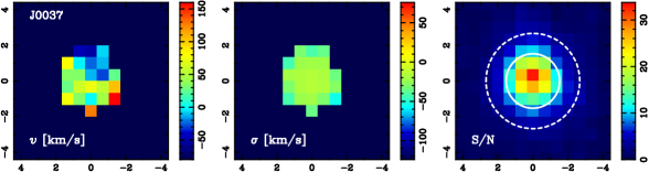
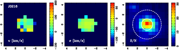
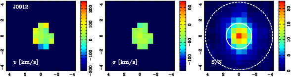
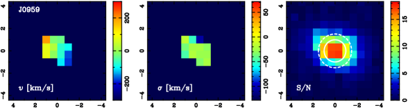
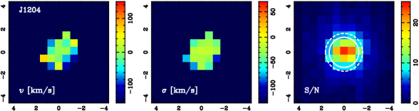
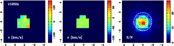
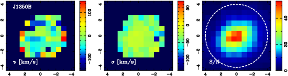
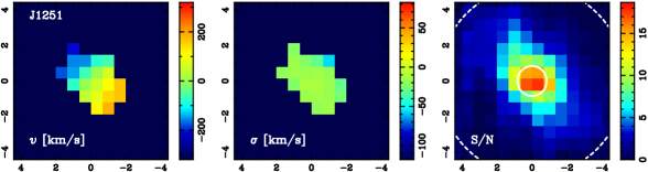
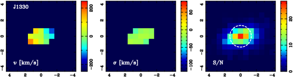
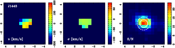
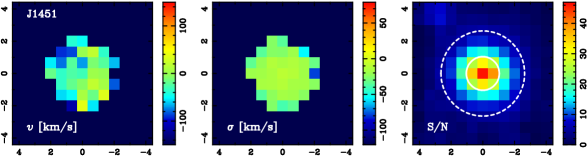
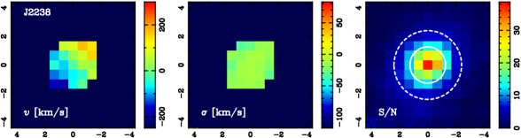
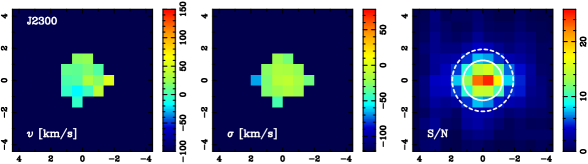
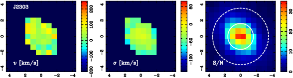
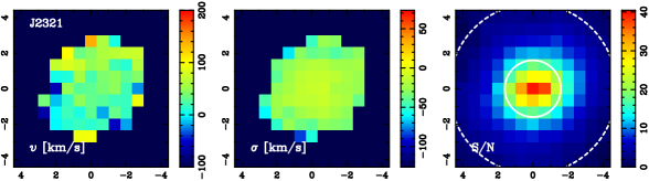
Figure 5: Results of kinematic analysis of the SLACS/IFU sample. For each target, the left plot shows the map of systematic velocity in the lens galaxy and the middle plot shows the map of velocity dispersion. All velocities refer to the rest frame of the lens galaxy. The right plots show the mean signal-to-noise ration (per pixel of width $0.65\,$Å) of the spectra. The axis labels are in arcsec. The maps are oriented such that north is to the top and east to the left.

The right panel compares measurements on the SDSS spectra to those on the VIMOS spectra, using identical methods. The different instrumental resolution ($R=1800$ for SDSS, $R=2500$ for VIMOS) has been taken into account. There appears to be a slight offset of the velocity dispersions obtained from the SDSS spectra compared to those from the VIMOS spectra. A similar trend is visible in the middle panel, while the comparison of the VIMOS measurements to the SDSS measurements from Bolton et al. (2008) does not show any offset.

Figure 6: Comparison of velocity dispersion measurements. The VIMOS spectra used here are summed over all spaxels within the same aperture as the SDSS spectra and analysed using our method (slacR). For the SDSS spectra, values measured with slacR and values obtained from Bolton et al. (2008, B08) are used.

6 Secondary sources

Some of the VIMOS/IFU fields in this sample contain objects in addition to the primary targets. For these fields we show larger-scale cut-outs from SDSS $r$-band images and label them by number. We extracted aperture spectra from the VIMOS data cubes and determined their redshifts by cross-correlation (Tonry & Davis, 1979) with a set of SDSS template spectra. Coordinates relative to the primary target and redshifts are listed in Table 3. The table also lists redshifts for the lens galaxies obtained by the same method in order to ensure that relative redshifts are accurate. Most of the additional objects are consistent with being at the same redshift as the lens galaxy.

Table 3: Data for additional sources in VIMOS/IFU fields. Coordinates are in arcsec relative to the position of the lens galaxy (always labelled as “1”) in each field. Redshifts marked with “?” are suggested by peaks in the cross-correlation but cannot be confirmed unambiguously by visual inspection. Objects with $z=0$ are stars.

Object	$\Delta\alpha\,(\arcsec)$	$\Delta\delta\,(\arcsec)$	z
J0216-1	$0$	$0$	0.3311
J0216-2	$+2.9$	$+3.2$	0.3327
J0216-3	$-0.9$	$-9.2$	0.3339
J0216-4	$-13.1$	$+3.5$	0.3327
J0216-5	$+12.4$	$+4.8$	0
J0912-1	0	0	0.1638
J0912-2	$+4.3$	$+6.4$	0.1609
J0935-1	$0$	$0$	0.3468
J0935-2	$+0.6$	$+5.2$	0.3407
J0935-3	$+8.6$	$-5.3$	0.3528
J1250B-1	$0$	$0$	0.0866
J1250B-2	$-5.1$	$+11.1$	0.2621?
J1251-1	$0$	$0$	0.2238
J1251-2	$+15.2$	$+10.8$	0
J1451-1	$0$	$0$	0.1248
J1451-2	$-10.5$	$-4.8$	0
J1451-3	$+2.9$	$+3.7$	0.5196?
J2238-1	$0$	$0$	0.1365
J2238-2	$+4.4$	$-4.6$	0.1358
J2300-1	$0$	$0$	0.2280
J2300-2	$-11.5$	$-7.1$	0.2277?

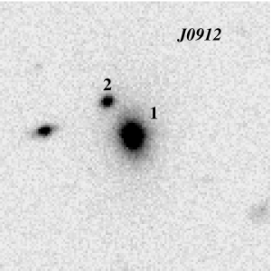
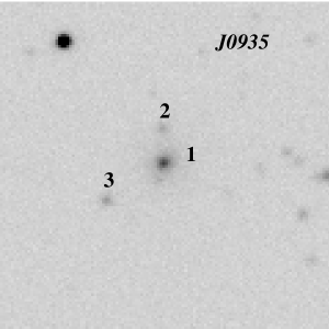
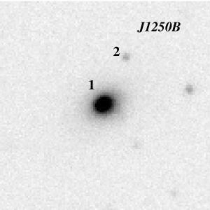
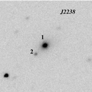
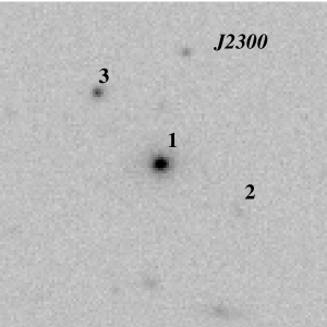
Figure 7: Finding charts for the sources listed in Table 3. Images are $r$-band images from the SDSS

7 Conclusions

In this paper, we have presented integral-field spectroscopic data obtained with VIMOS/IFU on a sample of 17 early-type lens galaxies selected from the SLACS survey. The data permit spatially resolved reconstruction of the stellar kinematics in these galaxies, presented as maps of systematic velocity and velocity dispersion. The sample, which spans a redshift range of $0.08$ to $0.35$ for the lens galaxies, is well-suited for a comparison with local samples, such as SAURON (Emsellem et al., 2004) and ATLAS^3D (Cappellari et al., 2011).

The distinction of slow-rotating and fast-rotating galaxies found in the SAURON sample (Emsellem et al., 2007) and earlier work (e.g. Davies et al., 1983) is also evident from the kinematic maps for our sample. About a third of the galaxies in the sample show clear evidence for rotation in their velocity maps.

While the spatial resolution of integral-field spectroscopic observations of galaxies at cosmological distances is necessarily much coarser than for local galaxies, the present sample offers the unique advantage that all the galaxies act as gravitational lenses and therefore offer the possibility to model their mass distribution using the two complementary methods of stellar dynamics and gravitational lensing. A Bayesian implementation of a fully self-consistent modelling algorithm for the joint analysis of stellar dynamics and gravitational lensing was developed by (Barnabè & Koopmans, 2007) and applied to subsets of this sample by Czoske et al. (2008) and Barnabè et al. (2009). Modelling and analysis of the full data set is presented in Barnabè et al. (2011).

Appendix A Estimation of noise vectors

Noise vectors can be estimated by following the reduction process from the initial raw data through the final data product. Using a model that takes into account photon noise (from object and sky) and readout noise, it is possible to express the variance in the data at each step in the reduction as a simple rescaling of the current intermediate data product.

The raw image frames have values $\mn@boldsymbol{d}$, expressed in ADU; these contain in addition to the useful data the bias $\mn@boldsymbol{b}$. The noise variance is the quadratic sum of the photon noise due to the data values $\mn@boldsymbol{d}-\mn@boldsymbol{b}$ and the readout noise $r$, given in electrons. In terms of electrons, the signal (without bias) is $(\mn@boldsymbol{d}-\mn@boldsymbol{b})/g$ and the variance is thus

$$\widehat{\sigma}_{\mathrm{raw}}^{2}=\frac{1}{g}\,(\mn@boldsymbol{d}-\mn@boldsymbol{b})+r^{2}\quad[\mathrm{e}^{-}].$$ (3)

The conversion from electrons to ADU is here given by the gain factor $g$ (in ADU/e^$-$).

Variance scale as

$$\sigma_{2}^{2}=c^{2}\sigma_{1}^{2}$$ (4)

when the data are rescaled according to $f_{2}=cf_{1}$. These relations preserve the signal-to-noise under rescaling. The variance of the raw images in terms of ADU is thus

$$\sigma_{\mathrm{raw}}^{2}=g\,(\mn@boldsymbol{d}-\mn@boldsymbol{b})+R^{2}\quad\mathrm{[ADU]},$$ (5)

where $R=gr$ is the readout noise in ADU.

The preliminary reduction step in vipgi subtracts the bias frame and produces BFC files. Compared to the raw frame, the variance is increased by the noise in the combined bias, $\sim R^{2}/5$. Since the readout noise is small anyway, we neglect this term.

$$\mathrm{BFC} = \mn@boldsymbol{d}-\mn@boldsymbol{b}$$ (6)

$$\sigma_{\mathrm{BFC}}^{2} = g\,\mathrm{BFC}+R^{2}\,.$$ (7)

The following reduction step applies the wavelength calibration, rectifies the two-dimensional spectra, and extracts one-dimensional spectra from these. The output files are names BFCEx. The EXR2D extension contains the rectified version of BFC. Neglecting the correlation of pixel noise introduced by the resampling, we have, as for the BFC:

$$\sigma_{\mathrm{EXR2D}}^{2}=g\,\mathrm{EXR2D}+R^{2}\,.$$ (8)

The 1D spectra in EXR1D are created from EXR2D by the Horne optimal extraction algorithm (Horne, 1986; Zanichelli et al., 2005), which sums over the spatial direction of the 2D spectrum using an estimate of the spatial profile of the light distribution as weights. The algorithm permits direct estimation of the noise variance in the extracted spectra; this is, however, not implemented in vipgi. We replace the Horne variance by the variance of a straight sum over $N_{c}=5$ columns in the 2D spectrum:

$$\mathrm{EXR1D} = \sum_{N_{\mathrm{c}}}\mathrm{EXR2D}$$ (9)

$$\sigma_{\mathrm{EXR1D}}^{2} = \sum_{N_{\mathrm{c}}}\sigma_{\mathrm{EXR2D}}^{2}=\sum_{N_{\mathrm{c}}}(g\,\mathrm{EXR2D}+R^{2})$$ (10)

$$= g\,\mathrm{EXR1D}+N_{c}R^{2}$$

Comparison of the noise predicted by Eq. (10) to real data in pure sky fibres (no object contribution) indicates that the noise is indeed somewhat overestimated, although not dramatically so.

The relative fibre transmissivity $t$ of a given fibre is estimated from the measured flux in a sky emission line and stored in a FITS table. Its application results in

$$\mathrm{EXR1DTC} = \frac{1}{t}\,\mathrm{EXR1D}$$ (11)

$$\sigma_{\mathrm{EXR1DTC}}^{2} = \frac{1}{t^{2}}\,\sigma_{\mathrm{EXR1D}}^{2}$$ (12)

$$= \frac{g}{t}\,\frac{1}{t}\,\mathrm{EXR1D}+\frac{N_{\mathrm{c}}}{t^{2}}\,R^{2}$$ (13)

$$= \frac{g}{t}\,\mathrm{EXR1DTC}+\frac{N_{\mathrm{c}}}{t^{2}}\,R^{2}\,.$$ (14)

The flux calibration uses the sensitivity function $s(\lambda)$. It acts like any other rescaling. The sensitivity function is normalized to an exposure time of $1\,\mathrm{s}$, hence it has to be rescaled to exposure time $T$ (in seconds). The estimate of the sky is based on a large number of fibers and has negligible effect on the variance.

$$\mathrm{EXR1DFLUX} = \frac{1}{Ts}\left(\mathrm{EXR1DTC}-\mathrm{SKY1D}\right)$$ (15)

$$\sigma_{\mathrm{EXR1DFLUX}}^{2} = \frac{g}{Tst}\,\frac{1}{Ts}\,\mathrm{EXR1DTC}+\frac{N_{\mathrm{c}}}{T^{2}s^{2}t^{2}}\,R^{2}$$ (16)

$$= \frac{g}{Tst}\,\overline{\mathrm{EXR1DFLUX}}+\frac{N_{c}}{T^{2}s^{2}t^{2}}\,R^{2}\,.$$ (17)

The overline indicates that the sky has not been subtracted.

The final data cube is generated by combining $N_{\mathrm{exp}}$ exposures using the median which results in a somewhat larger variance than the arithmetic mean. Simplifying again, we use the variance for the latter:

$$\mathrm{CUBE} \approx \frac{1}{N_{\mathrm{exp}}}\,\sum_{N_{\mathrm{exp}}}\mathrm{EXR1DFLUX}$$ (18)

$$\sigma_{\mathrm{CUBE}}^{2} \approx \frac{1}{N_{\mathrm{exp}}^{2}}\,\sum_{N_{\mathrm{exp}}}\sigma_{\mathrm{EXR1DFLUX}}^{2}$$ (19)

$$= \frac{1}{N_{\mathrm{exp}}^{2}}\,\sum_{\mathrm{N_{\mathrm{exp}}}}\frac{g}{Tst}\,\overline{\mathrm{EXR1DFLUX}}+\frac{N_{\mathrm{c}}}{N_{\mathrm{exp}}}\,\frac{R^{2}}{T^{2}s^{2}t^{2}}$$ (20)

$$= \frac{1}{N_{\mathrm{exp}}}\,\frac{g}{Tst}\,\overline{\mathrm{CUBE}}+\frac{N_{\mathrm{c}}}{N_{\mathrm{exp}}}\,\frac{R^{2}}{T^{2}s^{2}t^{2}}$$ (21)

Note that due to the dithering between exposures some of the spaxels in the cube arise from a combination of fibres from different quadrants which have different gain $g$ and sensitivity functions $s$. Assuming that we can use some effective values averaged over the four quadrants, the factor $g/st$ in the second row of Equation (19) can be taken out of the sum. This way, the variance of the cube can be obtained from a mock cube $\overline{\mathrm{CUBE}}$ which is produced in the same manner as the actual cube $\mathrm{CUBE}$, only with sky subtraction turned off.

All the parameters in Eq. (19) are stored as FITS header keywords or in table extensions of vipgi products.

In the final step, the global spectrum is created by summing over $N_{\mathrm{fib}}$ spaxels (defined by an aperture) in the final data cube, giving

$$\mathrm{SPEC} = \sum_{N_{\mathrm{fib}}}\,\mathrm{CUBE}$$ (22)

$$\sigma_{\mathrm{SPEC}}^{2} = \sum_{N_{\mathrm{fib}}}\sigma_{\mathrm{CUBE}}^{2}$$ (23)

$$= \frac{1}{N_{\mathrm{exp}}}\,\frac{g}{Tst}\,\sum_{N_{\mathrm{fib}}}\overline{\mathrm{CUBE}}+\frac{N_{\mathrm{fib}}N_{\mathrm{c}}}{N_{\mathrm{exp}}}\,\frac{g^{2}r^{2}}{T^{2}s^{2}t^{2}}$$ (24)

$$= \frac{1}{N_{\mathrm{exp}}}\,\frac{g}{Tst}\,\overline{\mathrm{SPEC}}+\frac{N_{\mathrm{fib}}N_{\mathrm{c}}}{N_{\mathrm{exp}}}\,\frac{g^{2}r^{2}}{T^{2}s^{2}t^{2}}$$ (25)

Equations (22) and (23) provide the recipes for the final spectrum. The readout noise $r$ is written in terms of electrons, as it usually is given in the fits headers.

References

- Auger et al. (2009) Auger M. W., Treu T., Bolton A. S., Gavazzi R., Koopmans L. V. E., Marshall P. J., Bundy K., Moustakas L. A., 2009, ApJ, 705, 1099
- Auger et al. (2010) Auger M. W., Treu T., Bolton A. S., Gavazzi R., Koopmans L. V. E., Marshall P. J., Moustakas L. A., Burles S., 2010, ApJ, 724, 511
- Auger et al. (2010) Auger M. W., Treu T., Gavazzi R., Bolton A. S., Koopmans L. V. E., Marshall P. J., 2010, ApJ, 721, L163
- Barnabè et al. (2010) Barnabè M., Auger M. W., Treu T., Koopmans L. V. E., Bolton A. S., Czoske O., Gavazzi R., 2010, MNRAS, 406, 2339
- Barnabè et al. (2011) Barnabè M., Czoske O., Koopmans L. V. E., Treu T., Bolton A. S., 2011, MNRAS, doi:10.1111/j.1365-2966.2011.18842.x
- Barnabè et al. (2009) Barnabè M., Czoske O., Koopmans L. V. E., Treu T., Bolton A. S., Gavazzi R., 2009, MNRAS, 399, 21
- Barnabè & Koopmans (2007) Barnabè M., Koopmans L. V. E., 2007, ApJ, 666, 726
- Barnabè et al. (2009) Barnabè M., Nipoti C., Koopmans L. V. E., Vegetti S., Ciotti L., 2009, MNRAS, 393, 1114
- Barnes (1992) Barnes J. E., 1992, ApJ, 393, 484
- Barth et al. (2002) Barth A. J., Ho L. C., Sargent W. L. W., 2002, AJ, 124, 2607
- Bernardi et al. (2003) Bernardi M., Sheth R. K., Annis J., Burles S., Finkbeiner D. P., Lupton R. H., Schlegel D. J., SubbaRao M., Bahcall N. A., et al., 2003, AJ, 125, 1882
- Bertin et al. (1994) Bertin G., Bertola F., Buson L. M., Danziger I. J., Dejonghe H., Sadler E. M., Saglia R. P., de Zeeuw P. T., Zeilinger W. W., 1994, A&A, 292, 381
- Bertola et al. (1993) Bertola F., Pizzella A., Persic M., Salucci P., 1993, ApJ, 416, L45
- Binney (1978) Binney J., 1978, MNRAS, 183, 501
- Blumenthal et al. (1984) Blumenthal G. R., Faber S. M., Primack J. R., Rees M. J., 1984, Nature, 311, 517
- Bolton et al. (2008) Bolton A. S., Burles S., Koopmans L. V. E., Treu T., Gavazzi R., Moustakas L. A., Wayth R., Schlegel D. J., 2008, ApJ, 682, 964
- Bolton et al. (2006) Bolton A. S., Burles S., Koopmans L. V. E., Treu T., Moustakas L. A., 2006, ApJ, 638, 703
- Cappellari & Emsellem (2004) Cappellari M., Emsellem E., 2004, Publ. Astr. Soc. Pac., 116, 138
- Cappellari et al. (2007) Cappellari M., Emsellem E., Bacon R., Bureau M., Davies R. L., de Zeeuw P. T., Falcón-Barroso J., Krajnović D., Kuntschner H., McDermid R. M., Peletier R. F., Sarzi M., van den Bosch R. C. E., van de Ven G., 2007, MNRAS, 379, 418
- Cappellari et al. (2011) Cappellari M., Emsellem E., Krajnović D., McDermid R. M., Scott N., Verdoes Kleijn G. A., Young L. M., Alatalo K., et al., 2011, MNRAS
- Carollo et al. (1995) Carollo C. M., de Zeeuw P. T., van der Marel R., Danziger I. J., Qian E. E., 1995, ApJ, 441, L25
- Colless et al. (2001) Colless M., Dalton G., Maddox S., Sutherland W., Norberg P., Cole S., Bland-Hawthorn J., Bridges T., et al., 2001, MNRAS, 328, 1039
- Corsini et al. (2008) Corsini E. M., Wegner G., Saglia R. P., Thomas J., Bender R., Thomas D., 2008, ApJS, 175, 462
- Czoske et al. (2009) Czoske O., Barnabè M., Koopmans L. V. E., 2009, in Giobbi G., et al. eds, Probing Stellar Populations out to the Distant Universe, Cefalù 2008 Vol. 1111 of AIP Conference Series. pp 137–140
- Czoske et al. (2008) Czoske O., Barnabè M., Koopmans L. V. E., Treu T., Bolton A. S., 2008, MNRAS, 384, 987
- Davies et al. (1983) Davies R. L., Efstathiou G., Fall S. M., Illingworth G., Schechter P. L., 1983, ApJ, 266, 41
- de Lorenzi et al. (2009) de Lorenzi F., Gerhard O., Coccato L., Arnaboldi M., Capaccioli M., Douglas N. G., Freeman K. C., Kuijken K., Merrifield M. R., Napolitano N. R., Noordermeer E., Romanowsky A. J., Debattista V. P., 2009, MNRAS, 395, 76
- Djorgovski & Davis (1987) Djorgovski S., Davis M., 1987, ApJ, 313, 59
- Dressler et al. (1987) Dressler A., Lynden-Bell D., Burstein D., Davies R. L., Faber S. M., Terlevich R., Wegner G., 1987, ApJ, 313, 42
- Eisenstein et al. (2001) Eisenstein D. J., Annis J., Gunn J. E., Szalay A. S., Connolly A. J., Nichol R. C., Bahcall N. A., Bernardi M., et al., 2001, AJ, 122, 2267
- Emsellem et al. (2011) Emsellem E., Cappellari M., Krajnovi’c D., Alatalo K., Blitz L., Bois M., Bournaud F., Bureau M., et al., 2011, MNRAS, 414, 888
- Emsellem et al. (2007) Emsellem E., Cappellari M., Krajnović D., van de Ven G., Bacon R., Bureau M., Davies R. L., de Zeeuw P. T., Falcón-Barroso J., Kuntschner H., McDermid R., Peletier R. F., Sarzi M., 2007, MNRAS, 379, 401
- Emsellem et al. (2004) Emsellem E., Cappellari M., Peletier R. F., McDermid R. M., Bacon R., Bureau M., Copin Y., Davies R. L., Krajnović D., Kuntschner H., Miller B. W., De Zeeuw P. T., 2004, MNRAS, 352, 721
- Faber et al. (2007) Faber S. M., Willmer C. N. A., Wolf C., Koo D. C., Weiner B. J., Newman J. A., Im M., Coil A. L., et al., 2007, ApJ, 665, 265
- Ferrarese & Merritt (2000) Ferrarese L., Merritt D., 2000, ApJ, 539, L9
- Gebhardt et al. (2000) Gebhardt K., Bender R., Bower G., Dressler A., Faber S. M. Filippenko A. V., Green R., Grillmair C., Ho L. C., Kormendy J., Lauer T. R., Magorrian J., Pinkney J., Richstone D., Tremaine S., 2000, ApJ, 539, L13
- Gerhard et al. (1998) Gerhard O., Jeske G., Saglia R. P., Bender R., 1998, MNRAS, 295, 197
- Gerhard et al. (2001) Gerhard O., Kronawitter A., Saglia R. P., Bender R., 2001, AJ, 121, 1936
- Grillo et al. (2008) Grillo C., Gobat R., Rosati P., Lombardi M., 2008, A&A, 477, L25
- Hopkins et al. (2006) Hopkins P. F., Hernquist L., Cox T. J., Di Matteo T., Robertson B., Springel V., 2006, ApJS, 163, 1
- Horne (1986) Horne K., 1986, Publ. Astr. Soc. Pac., 98, 609
- Illingworth (1977) Illingworth G., 1977, ApJ, 218, L43
- Keeton (2001) Keeton C. R., 2001, ApJ, 561, 46
- Kelson et al. (2000) Kelson D. D., Illingworth G. D., van Dokkum P. G., Franx M., 2000, ApJ, 531, 159
- Kochanek (2006) Kochanek C. S., 2006, in Meylan G., Jetzer P., North P., Schneider P., Kochanek C. S., Wambsganss J., eds, , Saas-Fee Advanced Course 33: Gravitational Lensing: Strong, Weak and Micro. Springer, pp 91–268
- Koopmans (2004) Koopmans L. V. E., 2004, in Dettmar R., Klein U., Salucci P., eds, Baryons in Dark Matter Halos
- Koopmans et al. (2009) Koopmans L. V. E., Bolton A. S., Treu T., Czoske O., Auger M. W., Barnabè M., Vegetti S., Gavazzi R., Moustakas L. A., Burles S., 2009, ApJ, 703, L51
- Koopmans & Treu (2002) Koopmans L. V. E., Treu T., 2002, ApJ, 568, L5
- Koopmans & Treu (2003) Koopmans L. V. E., Treu T., 2003, ApJ, 583, 606
- Koopmans et al. (2006) Koopmans L. V. E., Treu T., Bolton A. S., Burles S., Moustakas L. A., 2006, ApJ, 649, 599
- Le Fèvre et al. (2001) Le Fèvre O., Vettolani G., Maccagni D., Mancini D., Mazure A., Mellier Y., Picat J.-P., Arnaboldi M., et al., 2001, in Cristiani S., Renzini A., Williams R. E., eds, Deep Fields, Proceedings of the ESO/ECF/STScI Workshop held at Garching, Germany, 9-12 October 2000 The VIRMOS–VLT Deep Survey. p. 236
- Loewenstein & White (1999) Loewenstein M., White III R. E., 1999, ApJ, 518, 50
- Mamon & Łokas (2005) Mamon G. A., Łokas E. L., 2005, MNRAS, 362, 95
- Mehlert et al. (2000) Mehlert D., Saglia R. P., Bender R., Wegner G., 2000, A&AS, 141, 449
- R Development Core Team (2007) R Development Core Team 2007, R: A Language and Environment for Statistical Computing. R Foundation for Statistical Computing, Vienna, Austria
- Renzini (2006) Renzini A., 2006, ARAA, 44, 141
- Rix & White (1992) Rix H.-W., White S. D. M., 1992, MNRAS, 254, 389
- Romanowsky et al. (2003) Romanowsky A. J., Douglas N. G., Arnaboldi M., Kuijken K., Merrifield M. R., Napolitano N. R., Capaccioli M., Freeman K. C., 2003, Science, 301, 1696
- Saglia et al. (1993) Saglia R. P., Bertin G., Bertola F., Danziger J., Dejonghe H., Sadler E. M., Stiavelli M., de Zeeuw P. T., Zeilinger W. W., 1993, ApJ, 403, 567
- Saglia et al. (1992) Saglia R. P., Bertin G., Stiavelli M., 1992, ApJ, 384, 433
- Sandage & Visvanathan (1978) Sandage A., Visvanathan N., 1978, ApJ, 223, 707
- Scarlata et al. (2007) Scarlata C., Carollo C. M., Lilly S. J., Feldmann R., Kampczyk P., Renzini A., Cimatti A., Halliday C., et al., 2007, ApJS, 172, 494
- Scodeggio et al. (2005) Scodeggio M., Franzetti P., Garilli B., Zanichelli A., Paltani S., Maccagni D., Bottini D., Le Brun V., et al., 2005, Publ. Astr. Soc. Pac., 117, 1284
- Spiniello et al. (2011) Spiniello C., Koopmans L. V. E., Trager S. C., Czoske O., Treu T., 2011, arXiv:1103.4773, accecpted for publication in MNRAS
- Strauss et al. (2002) Strauss M. A., Weinberg D. H., Lupton R. H., Narayanan V. K., Annis J., Bernardi M., Blanton M., Burles S., et al., 2002, AJ, 124, 1810
- Thomas et al. (2007) Thomas J., Saglia R. P., Bender R., Thomas D., Gebhardt K., Magorrian J., Corsini E. M., Wegner G., 2007, MNRAS, 382, 657
- Tonry & Davis (1979) Tonry J., Davis M., 1979, AJ, 84, 1511
- Toomre & Toomre (1972) Toomre A., Toomre J., 1972, ApJ, 178, 623
- Trager et al. (2000) Trager S. C., Faber S. M., Worthey G., Jesús González J., 2000, AJ, 119, 1645
- Treu & Koopmans (2004) Treu T., Koopmans L. V. E., 2004, ApJ, 611, 739
- Treu et al. (2006) Treu T., Koopmans L. V. E., Bolton A. S., Burles S., Moustakas L., 2006, ApJ, 640, 662
- Valdes et al. (2004) Valdes F., Gupta R., Rose J. A., Singh H. P., Bell D. J., 2004, ApJS, 152, 251
- van der Marel & Franx (1993) van der Marel R. P., Franx M., 1993, ApJ, 407, 525
- Zanichelli et al. (2005) Zanichelli A., Garilli B., Scodeggio M., Franzetti P., Rizzo D., Maccagni D., Merighi R., Picat J.-P., et al., 2005, Publ. Astr. Soc. Pac., 117, 1271