Gravitational waves in dynamical spacetimes with matter content in the Fully Constrained Formulation

Abstract

The Fully Constrained Formulation (FCF) of General Relativity (GR) is a framework introduced as an alternative to the hyperbolic formulations traditionally used in numerical relativity. The FCF equations form a hybrid elliptic-hyperbolic system of equations including explicitly the constraints. We present an implicit-explicit numerical algorithm to solve the hyperbolic part, whereas the elliptic sector shares the form and properties with the well known Conformally Flat Condition (CFC) approximation. We show the stability and convergence properties of the numerical scheme with numerical simulations of vacuum solutions. We have performed the first numerical evolutions of the coupled system of hydrodynamics and Einstein equations within FCF. As a proof of principle of the viability of the formalism, we present 2D axisymmetric simulations of an oscillating neutron star. In order to simplify the analysis we have neglected the back-reaction of the gravitational waves (GWs) into the dynamics, which is small ($<2\%$) for the system considered in this work. We use spherical coordinates grids which are well adapted for simulations of stars and allow for extended grids that marginally reach the wave zone. We have extracted the GW signature and compared to the Newtonian quadrupole and hexadecapole formulae. Both extraction methods show agreement within the numerical errors and the approximations used ($\sim 30\%$).

I Introduction

Numerical relativity is a rather young branch of physics devoted to the numerical solution of Einstein equations for complex problems, mostly in theoretical astrophysics, which involve the evolution of spacetime and eventually the matter content of a system. It was born thanks to the theoretical advances which led to the 3+1 split of the Einstein equations Lichnerowicz44 ; CB52 popularized due to the work of ADM . The 3+1 split defines a foliation of spacetime which allows to solve the equations as an initial boundary value problem for a given spatial hypersurface which is then evolved in time.

Soon after that theoretical breakthrough, the first hydrodynamic calculations of the general-relativistic collapse of a star in spherical symmetry using a Lagrangian code were performed May66 ; May67 . Multidimensional simulations had to wait for the development of an Eulerian formulation Wilson72 which could overcome the problems of non-spherical Lagrangian codes. Those advances led to a tremendously prolific era of general relativistic hydrodynamics with multiple applications to the formation of black holes, accretion onto compact objects, binary neutron star mergers and core collapse supernovae (see Font08 for a recent review on the topic).

In parallel, a considerable effort was made to solve Einstein equations in vacuum. Only recently it has been possible to gain the sufficient understanding of the stability properties of numerical solutions of Einstein equations to overcome the numerical challenge of simulating the merger of two black holes and estimate its gravitational wave (GW) signal Pretorius05b . Despite the fact that some of the first successful simulations Pretorius05b ; Lindblom06 ; Szilagyi07 used the Generalized Harmonic formulation (GH) Friedrich85 ; Pretorius05a of Einstein equations (see more about GH below), most of the groups in the numerical relativity community make use of a different numerical recipe, resulting from the combination of different ingredients: i) the so-called BSSN formulation Baumgarte98 ; Shibata95 ; ii) the appropriate choice of gauge, with a slicing of the 1+log family and some variant of the hyperbolic Gamma-driver condition for the spatial gauge Bona95 ; Alcubierre03 ; vanMeter06 ; iii) the use of high order spatial methods (at least fourth-order); and iv) the use of high resolution due to the increasing computational power and development of adaptive mesh refinement (AMR) techniques. Using this recipe a number of groups Campanelli06 ; Baker06 ; Koppitz07 ; Herrmann07 ; Sperhake07 ; Bruegmann08 have provided waveforms of one of the most powerful sources of gravitational radiation in the Universe, the binary black hole merger. These events are one of the main candidates for the first direct detection of GWs in the ground-based GW observatories (LIGO, Virgo, GEO600, TAMA300).

According to the success of present formulations of the Einstein equations in different multidimensional scenarios, one could think that all the goals of numerical relativity have been achieved. Indeed, according to Shapiro86 , the Holy Grail of numerical relativity is a numerical code to solve Einstein equations, that simultaneously avoids singularities, handles black holes, maintains high accuracy, and runs forever. Current codes satisfy all the above requirements (with the exception, perhaps, of the last one), thanks to both the use of accurate numerical techniques and stable formulations of Einstein equations. There are, however, a number of problems that could arise when using such an homogeneous set of numerical recipes to solve a complex multidimensional numerical problem.

The first set of problems could be related to the homogeneity itself. All working formulations of Einstein equations consist in the solution of hyperbolic equations, and in most of the cases make use of the 3+1 decomposition of Einstein equations in a BSSN-like form, and use high order finite differences techniques to solve them numerically. This might make it difficult to detect fundamental theoretical problems in the set of equations to be solved.

Some work has appeared facing these questions. The original (as far as solving the binary black hole problem) article of Pretorius05b and some later ones Lindblom06 ; Szilagyi07 make use of GH formulation. It is a 4D covariant formulation which differs substantially from the 3+1 BSSN approach and allows for genuine comparisons between waveforms using different formulations Baker07 ; Hannam09 . Within the 3+1 decomposition of Einstein equations, some formulations have appeared Bona95 ; Alic11 in order to try to improve some of the weaknesses of the BSSN formulation, such as a better preservation of the constraints. An alternative is the characteristic approach (see WinicourLR for a review). The Cauchy-characteristic matching and extraction, based on a (2+1)+1 formulation, has been successfully used to accurately extract gravitational waves matching its evolution to interior Cauchy data Reisswig09 ; Babiuc11 ; Reisswig11 . However, the success in using this approach to simulate the whole spacetime is very limited Gomez98 ; Siebel02 due to the formation of coordinate caustics. Regarding the numerical methods, finite differences techniques have been used in all works, except for Lindblom06 in which pseudo-spectral methods were used, although no substantial differences have been found in comparison with finite differences codes Hannam09 . Nevertheless, an alternative to pure hyperbolic formulations of the Einstein equations, as the work that we present here, is interesting and desirable.

The second class of problems is related to the increasing level of complexity in the astrophysical scenarios that the community wants to simulate. After the binary black hole problem has been solved, the numerical relativity community is now concentrating more on the problem of solving non-vacuum spacetimes. The collapse of stellar cores and the merger of neutron stars represent challenges by itself, beyond the numerical evolution of Einstein equations: realistic microphysics, accurate multidimensional neutrino transport, magnetic fields, small scale instabilities (e.g., magnetorotational instability) and turbulence, non-ideal effects, elastic properties of the crust of neutron stars, superfluidity and superconductivity in cold neutron star interiors. Although full General Relativity (GR) is unavoidable in the case of the presence of black holes, approximations to GR in scenarios in which only neutron stars are present have a chance to simplify the numerical simulations to be able to understand the full physical complexity of those systems without the burden of solving the full GR equations.

The typical neutron star has a mass of about $M\sim 1.4M_{\odot}$ and a radius of $R\sim 10-15$ km, which results in a compactness of $GM/Rc^{2}\sim 0.2<1$. This implies that a post-Newtonian expansion of the gravitational field of an isolated neutron star is possible and convergent, and that the expected error in the dynamics of the system, if Newtonian gravity is used instead of full GR, is about $20\%$. However, it is well known that GR does not only produces quantitative effects in the dynamics of the system, but also qualitatively new effects like frame dragging or GWs. These two classes of effects appear at 1 and 2.5 post-Newtonian level, respectively (see e.g. Blanchet90 ), which represent changes in the dynamics of neutron stars of about $20\%$ and $<2\%$ at most. However, these effects can be important due to the non-linearity of the equations. As an example, in the case of neutron star binaries the energy loss due to GWs, despite their small nominal effect, make the orbit shrink until the neutron stars merge. In the case of the collapse of stellar cores, the stellar interior models used as progenitors can be treated safely in the Newtonian limit ($GM/Rc^{2}\sim 10^{-3}<<1$), and only as nuclear density is reached GR effects appear. In that case, it would be desirable to have numerical tools which could allow us to evolve efficiently and smoothly the spacetime, from the Newtonian regime of an stellar core to the mildly relativistic regime of a proto-neutron star or fully relativistic regime of a black hole.

An approximation to GR that could fill this gap between Newtonian gravity and GR is the Conformally Flat Condition (CFC) approximation (Isenberg ; WilsoM89 ). The main features of the CFC approximation are: i) although it is not a post-Newtonian approximation, it behaves as a 1PN theory Kley94 , and hence, it is possible to recover the Newtonian limit correctly in the case of weak gravity; ii) in spherical symmetry it coincides with GR, which makes it accurate for quasi-spherical objects like isolated neutron stars or for the collapse of stellar cores; iii) it only involves Poisson-like equations for the spacetime, and therefore the numerical methods and computational costs are closer to Newtonian simulations than to full GR simulations; and iv) it neglects GWs and the energy losses related to them. The numerical solution of elliptic equations is more involved than hyperbolic equations. However, the time-step in CFC is limited by the sound speed instead of the speed of light, as in the case of hyperbolic formulations of GR. That provides a considerably speed up in many scenarios that widely overcomes the extra cost of solving elliptic equations, making the numerical evolution considerably faster. The CFC approximation was originally thought to deal with the neutron star binary case Wilson96 ; Oechslin02 ; Faber04 ; Oechslin07 . In this case, energy losses by GWs have to be included as an extra ingredient to allow for the neutron stars to merge. The major success, however, has been in the collapse of stellar cores (Dimmelmeier01 ; Dimmelmeier02a ; Dimmelmeier02b ), which lead to the computation of GW emission using physically motivated microphysics Dimmelmeier09 , magnetic fields CerdaDuran08 , and neutrino transport Mueller10 . The CFC approach has also been successfully used to simulate the phase-transition-induced collapse of rotating neutron stars to hybrid quark stars Abdikamalov09 and the evolution of equilibrium models of rotating neutron stars Cook96 ; Dimmelmeier06 . Direct comparisons of the CFC approach with full GR have shown that differences between both approaches, in the case of core collapse, are smaller than the numerical differences between the codes Shibata04 ; Ott07a ; Ott07b . This fact is understandable since the next post-Newtonian corrections to CFC were found to have an impact on the non-linear dynamics of less than $1\%$ CerdaDuran05 . In the case of neutron star mergers we are not aware of a direct comparison between CFC and full GR.

A new formulation of Einstein equations which could address both classes of problems mentioned above, and share some properties with the CFC approximation, is the Fully Constrained Formulation (FCF) Bonazzola04 . This formulation is based on the 3+1 split of Einstein equations but different from all other formulations of Einstein equations that are purely hyperbolic, the FCF maximizes the number of elliptic equations by solving the constraint equations at each time-step and choosing an appropriate gauge condition. As a consequence, the hyperbolic part of FCF only contains two degrees of freedom, which correspond, far from the matter sources, to the GW content of the system. Therefore, FCF is fundamentally different from fully hyperbolic formulations of GR and can be used as another check of the consistency of the numerical solutions of Einstein equations. There are other formulations which incorporate the constraints into the evolution system (see JarValGou08 , section 5.2.2., for most relevant examples); however, no numerical simulations have been performed yet with most of them (e.g., AnMon ), or simulations are restricted to axisymmetric spacetimes (e.g., Rinne ). Moreover, FCF is a natural generalization of the CFC approximation; this fact makes possible a natural extension of all the numerical codes which use this approximation, in order to have a proper treatment of the gravitational radiation of the system without too much effort. It also creates a bridge between weak gravity systems, which are well described within the CFC approximation, and the strong gravity limit.

In practice, to extend a CFC code to FCF one has to add additional hyperbolic equations to the existing CFC elliptic equations (and also some extra sources in these elliptic equations). This evolution system, written as a first-order one, is a hyperbolic system CC08b and includes the whole hyperbolic sector of the metric of spacetime in this formulation. In particular, the explicit values of the eigenvalues and eigenvectors of the hyperbolic metric system allow to guarantee the expected physical behavior on trapping horizons CC08a . The remaining metric variables form the elliptic sector, which is similar to the group of elliptic equations in the CFC approximation, with extra sources. Recent works CC09 overcome some pathological problems related with non-local uniqueness in the elliptic equations in CFC, and also in FCF. The equations were rewritten in such a way that these problems were solved, and the new scheme has been used successfully in some applications Mueller10 ; BucZan ; BausThesis .

The analysis of the numerical evolution of the hyperbolic metric system is the main objective of this work, including aspects like numerical stability of the system in long-term simulations, evolution of equilibrium configurations, or the influence of the elliptic equations in the system. We perform all the numerical simulations using the CoCoNuT code Dimmelmeier02a ; Dimmelmeier02b ; Dimmelmeier05 , which was originally designed to evolve the hydrodynamics equations in the dynamical spacetime of the CFC approximation. The code uses spherical coordinates for the evolution of both matter and spacetime; this is very convenient in the present work, since it allows us to place the outer boundary sufficiently far from the star, in order to perform an accurate GW extraction CC10 .

In this paper we present the first accurate extraction of the gravitational wave signature coming from the evolution of rotating oscillating neutron stars within FCF. As a first step towards a full evolution of the coupled system of elliptic and hyperbolic equations of the FCF, we have neglected the back-reaction of the GWs onto the dynamics of the system, which is a justified approximation in the case of isolated neutron stars and the collapse of stellar cores.

The article is organized as follows. In Sec. II we review the FCF and detail the formulation used in the evolution of spacetime. In Sec. III we describe the numerical methods used in the evolution of the different systems of equations (hydrodynamics, elliptic and hyperbolic metric equations). In Sec. IV we test our numerical implementation through the evolution of a vacuum spacetime with analytical solution. In Sec. V we perform simulations of equilibrium configurations of rotating neutron star and extract GWs from perturbed oscillating models. Conclusions are drawn in Sec. V. Throughout the paper we use the signature $(-,+,+,+)$ for the spacetime metric, and units in which $c=G=M_{\odot}=1$. Greek indices run from 0 to 3, whereas Latin ones from 1 to 3 only.

II Spacetime evolution

II.1 Fully Constrained Formalism

Given an asymptotically flat spacetime $({\cal M},g_{\mu\nu})$ we consider a $3+1$ splitting by spacelike hypersurfaces $\Sigma_{t}$, denoting timelike unit normals to $\Sigma_{t}$ by $n^{\mu}$. The spacetime on each spacelike hypersurface $\Sigma_{t}$ is described by the pair $(\gamma_{ij},K^{ij})$, where $\gamma_{\mu\nu}=g_{\mu\nu}+n_{\mu}n_{\nu}$ is the Riemannian metric induced on $\Sigma_{t}$. We choose the convention $K_{\mu\nu}=-\frac{1}{2}{\cal L}_{\bm{n}}\gamma_{\mu\nu}$ for the extrinsic curvature. With the lapse function $N$ and the shift vector $\beta^{i}$, the Lorentzian metric $g_{\mu\nu}$ can be expressed in coordinates $(x^{\mu})$ as

$$g_{\mu\nu}\,dx^{\mu}\,dx^{\nu}=-N^{2}\,dt^{2}+\gamma_{ij}(dx^{i}+\beta^{i}\,dt)(dx^{j}+\beta^{j}\,dt).$$ (1)

As in Bonazzola04 we introduce a time independent flat metric $f_{ij}$, which satisfies ${\cal L}_{\bm{t}}f_{ij}=\partial_{t}f_{ij}=0$ and coincides with $\gamma_{ij}$ at spatial infinity. We define $\gamma:=\det\gamma_{ij}$ and $f:=\det f_{ij}$. We introduce the following conformal decomposition of the spatial metric $\gamma_{ij}$:

$$\gamma_{ij}=\psi^{4}\tilde{\gamma}_{ij},\qquad\psi=(\gamma/f)^{1/12}.$$ (2)

The deviation of the conformal metric from the flat fiducial one is denoted by $h^{ij}$,

$$h^{ij}:=\tilde{\gamma}^{ij}-f^{ij}.$$ (3)

Once the $3+1$ conformal decomposition is performed, a choice of gauge is needed in order to properly reformulate Einstein equations. The prescriptions in Bonazzola04 are maximal slicing,

$$K=0,$$ (4)

and the so-called generalized Dirac gauge,

$${\cal D}_{i}\tilde{\gamma}^{ij}={\cal D}_{i}h^{ij}=0,$$ (5)

where $K=\gamma^{ij}K_{ij}$ denotes the trace of the extrinsic curvature and ${\cal D}_{k}$ stands for the Levi–Civita connection associated with the flat metric $f_{ij}$. More details can be found in Bonazzola04 . Einstein equations then become a coupled elliptic-hyperbolic system: the elliptic sector acts on the variables $\psi$, $N$, and $\beta^{i}$, and the hyperbolic sector acts on $h^{ij}$. More details of the analysis carried out for both elliptic and hyperbolic systems can be found in CC08b ; CC09 .

We introduce the conformal decomposition

$$\hat{A}^{ij}:=\psi^{10}K^{ij},$$ (6)

and its decomposition in longitudinal and transverse-traceless parts

$$\hat{A}^{ij}=(LX)^{ij}+\hat{A}^{ij}_{\rm TT},$$ (7)

where

$$(LX)^{ij}:={\cal D}^{i}X^{j}+{\cal D}^{j}X^{i}-\frac{2}{3}f^{ij}{\cal D}_{k}X^{k}$$ (8)

and ${\cal D}_{i}\hat{A}^{ij}_{\rm TT}=0$. These decompositions are motivated by the local uniqueness properties of elliptic equations shown in CC09 . We define $w^{ij}_{k}:={\cal D}_{k}\tilde{\gamma}^{ij}$. The hyperbolic system for $h^{ij}$ can be written as a first-order evolution system for the tensors $\left(h^{ij},\hat{A}^{ij},w^{ij}_{k}\right)$,

$$\frac{\partial h^{ij}}{\partial t} = 2N\psi^{-6}\hat{A}^{ij}+\beta^{k}w^{ij}_{k}-\tilde{\gamma}^{ik}{\cal D}_{k}\beta^{j}-\tilde{\gamma}^{kj}{\cal D}_{k}\beta^{i}+\frac{2}{3}\tilde{\gamma}^{ij}{\cal D}_{k}\beta^{k},$$ (9)

$$\frac{\partial\hat{A}^{ij}}{\partial t} = {\cal D}_{k}\left(\frac{N\psi^{2}}{2}\tilde{\gamma}^{kl}w^{ij}_{l}+\beta^{k}\hat{A}^{ij}\right)-\hat{A}^{kj}{\cal D}_{k}\beta^{i}-\hat{A}^{ik}{\cal D}_{k}\beta^{j}+\frac{2}{3}\hat{A}^{ij}{\cal D}_{k}\beta^{k}+2N\psi^{-6}\tilde{\gamma}_{kl}\hat{A}^{ik}\hat{A}^{jl}$$ (10)

$$-8\pi N\psi^{6}\left(\psi^{4}S^{ij}-\frac{S\tilde{\gamma}^{ij}}{3}\right)+N\left(\psi^{2}\tilde{R}_{*}^{ij}+8\tilde{\gamma}^{ik}\tilde{\gamma}^{jl}{\cal D}_{k}\psi{\cal D}_{l}\psi\right)+4\psi\left(\tilde{\gamma}^{ik}\tilde{\gamma}^{jl}{\cal D}_{k}\psi{\cal D}_{l}N+\tilde{\gamma}^{ik}\tilde{\gamma}^{jl}{\cal D}_{k}N{\cal D}_{l}\psi\right)$$

$$-\frac{1}{3}\left[N\left(\psi^{2}\tilde{R}+8\tilde{\gamma}^{kl}{\cal D}_{k}\psi{\cal D}_{l}\psi\right)+8\psi\tilde{\gamma}^{kl}{\cal D}_{k}\psi{\cal D}_{l}N\right]\tilde{\gamma}^{ij}$$

$$-\frac{1}{2}\left(\tilde{\gamma}^{ik}w^{lj}_{k}+\tilde{\gamma}^{kj}w^{il}_{k}\right){\cal D}_{l}(N\psi^{2})-\tilde{\gamma}^{ik}\tilde{\gamma}^{jl}{\cal D}_{k}{\cal D}_{l}(N\psi^{2})+\frac{1}{3}\tilde{\gamma}^{ij}\tilde{\gamma}^{kl}{\cal D}_{k}{\cal D}_{l}(N\psi^{2}),$$

$$\frac{\partial w^{ij}_{k}}{\partial t} = {\cal D}_{k}\left(2N\psi^{-6}\hat{A}^{ij}+\beta^{l}w^{ij}_{l}-\tilde{\gamma}^{il}{\cal D}_{l}\beta^{j}-\tilde{\gamma}^{lj}{\cal D}_{l}\beta^{i}+\frac{2}{3}\tilde{\gamma}^{ij}{\cal D}_{l}\beta^{l}\right)\,\,$$ (11)

where

$$\tilde{R} = \frac{1}{4}\tilde{\gamma}^{kl}{\cal D}_{k}h^{mn}{\cal D}_{l}\tilde{\gamma}_{mn}-\frac{1}{2}\tilde{\gamma}^{kl}{\cal D}_{k}h^{mn}{\cal D}_{n}\tilde{\gamma}_{ml},$$ (12)

$$\tilde{R}_{*}^{ij} = \frac{1}{2}\left[-w_{l}^{ik}w_{k}^{jl}-\tilde{\gamma}_{kl}\tilde{\gamma}^{mn}w_{m}^{ik}w_{n}^{jl}+\tilde{\gamma}_{nl}w_{k}^{mn}\left(\tilde{\gamma}^{ik}w_{m}^{jl}+\tilde{\gamma}^{jk}w_{m}^{il}\right)\right]+\frac{1}{4}\tilde{\gamma}^{ik}\tilde{\gamma}^{jl}w_{k}^{mn}{\cal D}_{l}\tilde{\gamma}_{mn},$$ (13)

$S_{ij}:=T_{\mu\nu}\gamma^{\mu}_{i}\gamma^{\nu}_{j}$ is the stress tensor and $S:=\gamma^{ij}S_{ij}$ is its trace, $T_{\mu\nu}$ being the energy-momentum tensor, measured by the observer of 4-velocity $n^{\mu}$ (Eulerian observer). Moreover, the system obeys the constraint of the Dirac gauge, $w^{ij}_{i}=0$, and for the determinant of the conformal metric, we obtain $\tilde{\gamma}=f$.

The elliptic part of the FCF equations can be rewritten as

$$\tilde{\gamma}^{kl}{\cal D}_{k}{\cal D}_{l}\psi = -2\pi\psi^{-1}E^{*}-\frac{\tilde{\gamma}_{il}\tilde{\gamma}_{jm}\hat{A}^{lm}\hat{A}^{ij}}{8\psi^{7}}+\frac{\psi\tilde{R}}{8},$$ (14)

$$\tilde{\gamma}^{kl}{\cal D}_{k}{\cal D}_{l}(N\psi) = \left[2\pi\psi^{-2}(E^{*}+2S^{*})+\left(\frac{7\tilde{\gamma}_{il}\tilde{\gamma}_{jm}\hat{A}^{lm}\hat{A}^{ij}}{8\psi^{8}}+\frac{\tilde{R}}{8}\right)\right](N\psi),$$ (15)

$$\tilde{\gamma}^{kl}{\cal D}_{k}{\cal D}_{l}\beta^{i}\!+\frac{1}{3}\tilde{\gamma}^{ik}{\cal D}_{k}{\cal D}_{l}\beta^{l} = 16\pi N\psi^{-6}\tilde{\gamma}^{ij}(S^{*})_{j}+\hat{A}^{ij}{\cal D}_{j}\left(2N\psi^{-6}\right)-2N\psi^{-6}\Delta^{i}_{kl}\hat{A}^{kl},$$ (16)

where $E:=T_{\mu\nu}n^{\mu}n^{\nu}$ and $S_{i}:=-\gamma^{\mu}_{i}T_{\mu\nu}n^{\nu}$ are, respectively, the energy density and the momentum density measured by the observer of 4-velocity $n^{\mu}$, $E^{*}:=\psi^{6}E$, $S^{*}:=\psi^{6}S$, $(S^{*})_{i}:=\psi^{6}S_{i}$, and

$$\Delta^{k}_{ij}=\frac{1}{2}\tilde{\gamma}^{kl}\left({\cal D}_{i}\tilde{\gamma}_{lj}+{\cal D}_{j}\tilde{\gamma}_{il}-{\cal D}_{l}\tilde{\gamma}_{ij}\right).$$ (17)

The decomposition introduced in Eq. (7) leads to an extra elliptic equation for the vector $X^{i}$,

$${\cal D}_{j}{\cal D}^{j}X^{i}+\frac{1}{3}{\cal D}^{i}{\cal D}_{k}X^{k}+\tilde{\gamma}^{im}\left({\cal D}_{k}\tilde{\gamma}_{ml}-\frac{{\cal D}_{m}\tilde{\gamma}_{kl}}{2}\right)(LX)^{kl}$$

$$\qquad=8\pi\tilde{\gamma}^{ij}(S^{*})_{j}-\tilde{\gamma}^{im}\left({\cal D}_{k}\tilde{\gamma}_{ml}-\frac{{\cal D}_{m}\tilde{\gamma}_{kl}}{2}\right)\hat{A}_{\mathrm{TT}}^{kl},$$ (18)

and the evolution Eq. (10) can be viewed as an evolution equation for the tensor $\hat{A}^{ij}_{\rm TT}$.

More details about the derivation of all the equations can be found in CC09 . All these equations are to be solved coupled with the hydrodynamic equations for the evolution of matter which can be derived from the Bianchi identities and the continuity equation,

$$T^{\mu\nu}_{;\mu}=0\qquad J^{\mu}_{;\mu}=0.$$ (19)

Explicit expressions for the hydrodynamics equations for the case of a perfect fluid in the form that it is used in the present work can be found in Dimmelmeier05 .

II.2 Passive FCF

	hydrodynamics	elliptic metric	hyperbolic
Approach	equations	sector	metric sector
CFC	Dimmelmeier02a	(20)-(23)	no
Passive FCF	Dimmelmeier02a	(20)-(23)	(9)-(11)
FCF	Ibanez2000	(14)-(16), (18)	(9)-(11)
Teukolsky waves	no (vacuum)	fixed Minkowsky	(9)-(11)
Equilibrium NS	fixed, lapming06	fixed, lapming06	(9)-(11)
Oscillating NS	Dimmelmeier02a	(20)-(23)	(9)-(11)

Table 1: Guide to the approaches to GR used in this work: first three rows represent the approaches discussed in the theoretical part of the present work and the last three rows the approaches used in the numerical part. For each approach we provide the equations that we use for each of the three sectors (hydrodynamics, elliptic and hyperbolic metric sectors), a suitable reference where the equations can be found or a comment.

An interesting property of the fully constrained formalism is that if $h^{ij}=0$, the resulting 3-metric $\gamma_{ij}$ is conformally flat. This condition corresponds to the well know conformally flat condition (CFC) approximation Isenberg ; WilsoM89 of Einstein equations. The CFC approximation has been proved to provide accurate evolutions of spacetimes including single neutron stars and core collapse supernovae Shibata04 ; Ott07a ; Ott07b . In these scenarios the back-reaction of the GWs on the dynamics of the system is so small that $h^{ij}$ can be approximated to be zero. The main drawback of the CFC approximation is that the GW content is removed from the system, and the computation of the GW emission has to be performed approximately by means of the quadrupole formula.

Since our aim is to deal with this kind of astrophysical scenarios, neutron stars and core collapse supernovae, in which the GWs are not important for the dynamics, when solving the complete FCF system, the back-reaction of the $h^{ij}$ tensor onto the hydrodynamics and elliptic part of the metric equations can be neglected. Therefore, we impose $h^{ij}=0$ in Eqs. (14)–(18). The resulting system of elliptic equations

$$\Delta\psi = -2\pi\psi^{-1}E^{*}-\frac{f_{il}f_{jm}\hat{A}^{lm}\hat{A}^{ij}}{8\psi^{7}},$$ (20)

$$\Delta(N\psi) = 2\pi N\psi^{-1}(E^{*}+2S^{*})$$ (21)

$$+ N\psi^{-7}\frac{7f_{il}f_{jm}\hat{A}^{lm}\hat{A}^{ij}}{8},$$

$$\Delta\beta^{i}\! + \frac{1}{3}f^{ij}{\cal D}_{j}{\cal D}_{k}\beta^{k}={\cal D}_{j}\left(2N\psi^{-6}\hat{A}^{ij}\right),$$ (22)

$$\Delta X^{i} + \frac{1}{3}f^{ij}{\cal D}_{j}{\cal D}_{k}X^{k}=8\pi{f}^{ij}(S^{*})_{j}$$ (23)

is identical to the CFC equations in the form described in CC09 .

In the present work we solve the coupled evolution of the hyperbolic system for $h^{ij}$ given by Eqs. (9)–(11), the elliptic approximated system for $N$, $\psi$ and $\beta^{i}$, given by Eqs. (20)–(22) and the hydrodynamics equations. We call the new system passive FCF, in the sense that we neglect the back-reaction of the GWs onto the dynamics of the system. Contrary to the CFC approximation, this approach does not neglect the GWs itself. Therefore, it allows one to compute the GW emission of the system directly from the spacetime evolution. Upper three rows of table 1 summarize the approximations used in the case of CFC, passive FCF and FCF.

III Numerical methods

We perform all the simulations of this work using the numerical code CoCoNuT Dimmelmeier02a ; Dimmelmeier05 ; coconut . We have extended this code, which solves the coupled evolution of the hydrodynamics equations with spacetime evolution in the CFC approximation, to add the new degrees of freedom necessary for the FCF in the passive FCF approximation. In the following, we briefly describe the numerical methods used in the code to solve the hydrodynamics equations and the elliptic part of the FCF formalism. These methods and equations are identical to those described in Dimmelmeier05 ; CC09 . We also describe the numerical techniques applied to solve the evolution of the $h^{ij}$ tensor, which is necessary to extend the CFC approximation to passive FCF. In all cases we consider spherical coordinates and axisymmetry. In order to simplify the notation, we will refer to the three sets of variables as hydrodynamics variables, ${\bf U}:=(D,S_{i},\tau)$ (see definitions below), elliptic-spacetime variables or CFC variables, ${\bf V}:=(N,\psi,\beta^{i},X^{i})$, and hyperbolic spacetime variables, ${\bf W}:=(h^{ij},\hat{A}^{ij},w^{ij}_{k})$.

III.1 Hydrodynamics equations

The system of Eqs. (19) can be cast into a system of conservation laws Ibanez2000 as

$$\partial_{t}{\bf U}+\partial_{i}{\bf F}^{i}({\bf U},{\bf V})=Q({\bf U},{\bf V}).$$ (24)

${\bf U}:=(D,S_{i},\tau)$ is the conserved variables vector, $D\equiv-J^{\mu}n_{\mu}$ and $\tau\equiv E-D$.

Since we are neglecting the back-reaction of the GWs onto the dynamics of the fluid, there is no dependence on the hyperbolic-spacetime variables ${\bf W}$ in the previous set of equations. We use Godunov-type schemes, which are suitable for solving equations written in conservative form. These schemes allow for a numerical evolution of the system with high accuracy in conservation of mass, momentum and energy, and the correct behavior at discontinuities, e.g. shock waves at the surface of neutron stars (see e.g. Font08 ). We use the Marquina flux formula Donat1998 combined with a second-order linear reconstruction with monotonized central slope limiter Toro99 . The time update of the matter quantities relies on the method of lines in combination with a second-order accurate explicit Runge-Kutta scheme. The time step is restricted by the Courant-Friedrich-Lewi (CFL) condition CFL1928 . This combination provides second-order convergence in a number of tests including the evolution of oscillating neutron stars Dimmelmeier05 , which degrades to first-order in the presence of discontinuities. We use spherical coordinates $(r,\theta,\varphi)$ in axisymmetry. The angular grid is equally spaced in $\theta$, but the radial grid can be non-equidistant.

III.2 Elliptic spacetime equations

Once the values of the hydrodynamic variables, $\bf U$, have been updated, the CFC metric, $\bf V$, can be updated by solving the elliptic part of the spacetime evolution equations. It consists in a system of Poisson-like elliptic equations, Eqs. (20)–(22), which can be written as

$$\Delta{\bf V}=f({\bf U},{\bf V}).$$ (25)

This system of equations can be solved hierarchically, following the procedure described in CC09 .

We compute the numerical solution using spectral methods. The sources of the equations are interpolated (parabolic interpolation) from the finite difference grid to the spectral one, where the elliptic equations are solved using the LORENE library for spectral methods Lorene . The spectral solution of the equations is evaluated at the finite difference grid in order to update the metric fields $N$, $\psi$ and $\beta^{i}$, which are needed for the recovery of the primitive hydrodynamic variables (e.g., density and velocity) and the evolution of $h^{ij}$ (see next subsection). The spectral grid consists of several radial domains in spherical coordinates. Further details can be found in Dimmelmeier05 .

Since the system of equations is elliptic, the Courant condition does not restrict the time step. Although the metric could be computed after every time step, in some scenarios the typical time scale of variation of the CFC variables is much longer than that of the hydrodynamic ones, and it is justified to compute ${\bf V}$ not at every hydrodynamics time step. In the simulations of neutron star oscillations presented in this paper we compute the CFC part of the metric every 10th hydrodynamical time steps and use a parabolic extrapolation between consecutive metric computations. This method has shown to provide sufficient accuracy for this scenario Dimmelmeier02a .

III.3 Hyperbolic spacetime equations

Once we have updated the hydrodynamic variables, $\bf U$, and the CFC variables, $\bf V$, we solve the hyperbolic part of the spacetime evolution, Eqs. (9)–(11). This part contains the gravitational wave information of the system. It consists of evolution equations for the variables $\bf W$ of the form

$$\partial_{t}{\bf W}=g({\bf W},{\bf V},{\bf U}).$$ (26)

We solve the system following a two step approach. In the first step we update $h^{ij}$ and $\hat{A}^{ij}$ to the next hypersurface, $\Sigma_{t^{n+1}}\equiv\Sigma_{t^{n}+\Delta t}$, denoted by an upperindex $(n+1)$, using only information of the previous hypersurface, $\Sigma_{t^{n}}$, denoted by $(n)$. It is therefore an explicit algorithm of the form

$$\partial_{t}h^{ij} = S_{h}(h^{ij(n)},\hat{A}^{ij(n)},w^{ij(n)}_{k},{\bf V}^{(n)}),$$ (27)

$$\partial_{t}\hat{A}^{ij} = S_{\hat{A}}(h^{ij(n)},\hat{A}^{ij(n)},w^{ij(n)}_{k},{\bf U}^{(n)},{\bf V}^{(n)}),$$ (28)

which can be integrated using explicit Runge-Kutta schemes.

In the second step we update $w^{ij}_{k}$ using an implicit-explicit approach. We compute the sources using the values $(h^{ij(n)},\hat{A}^{ij(n)})$ and the updated values of $(h^{ij(n+1)},\hat{A}^{ij(n+1)})$ computed in the first step. The sources of Eq. (11) can be splitted into two terms of the form

$$\partial_{t}w^{ij}_{k}=S_{w1}(h^{ij},\hat{A}^{ij},{\bf V})+S_{w2}(w^{ij}_{k},{\bf V}),$$ (29)

where

$$S_{w1} = {\cal D}_{k}\left(2N\psi^{-6}\hat{A}^{ij}-\tilde{\gamma}^{il}{\cal D}_{l}\beta^{j}-\tilde{\gamma}^{lj}{\cal D}_{l}\beta^{i}+\frac{2}{3}\tilde{\gamma}^{ij}{\cal D}_{l}\beta^{l}\right),$$

$$S_{w2} = {\cal D}_{k}\left(\beta^{l}w^{ij}_{l}\right).$$ (30)

The first term, $S_{w1}$, does not depend explicitly on the evolved variables $w^{ij}_{k}$. The second term, $S_{w2}$, depends linearly on $w^{ij}_{k}$ and does not depend explicitly on the variables $(h^{ij},\hat{A}^{ij})$. This property allows us to design a numerical algorithm to evolve $w^{ij}_{k}$ from $\Sigma_{t^{n}}$ to $\Sigma_{t^{n+1}}$, using the values of $h^{ij}$ and $\hat{A}^{ij}$ at $\Sigma_{t^{n+1}}$ and all other variables at $\Sigma_{t^{n}}$, i.e.,

$$\partial_{t}w^{ij}_{k}=S_{w1}(h^{ij(n+1)},\hat{A}^{ij(n+1)},{\bf V}^{(n)})+S_{w2}(w^{ij(n)}_{k},{\bf V}^{(n)}).$$ (31)

This scheme provides a numerically stable evolution, due to the (partially) implicit dependence on $S_{w1}$ and explicit on $S_{w2}$. We evolve the system with the same Runge-Kutta schemes as in the first step, but with the corresponding partially implicit evaluation of the $S_{w1}$ source term (see Appendix A for more details). However, this evaluation reduces the theoretical order of the scheme, which is observed in numerical simulations in those scenarios where the terms $S_{w1}(h^{ij(n+1)},\hat{A}^{ij(n+1)},{\bf V}^{(n)})$ and $S_{w1}(h^{ij(n)},\hat{A}^{ij(n)},{\bf V}^{(n)})$ differ significantly. In practice, the reduction of the order of the method can be small as long as the leading term of the sources for the evolution of $w^{ij}_{k}$ is the one containing the $\hat{A}^{ij}$ tensor, as we have obtained in the evolution of Teukolsky waves with a method based on a fourth-order Runge-Kutta scheme (see Sec. IV). In other cases the order of convergence of the method can reduce up to second-order within the same scheme, as we have obtained when the tensor $h^{ij}$ reaches stationary values in the evolution of equilibrium configurations of rotating neutron stars (see Sec. V.2). In a general scenario, an implicit-explicit (IMEX) Runge-Kutta scheme AsRuuSpi ; PaRu could be used to prevent the reduction of the order of convergence, although this is beyond the scope of this paper. The use of implicit terms for the second step of the time integration is crucial in order to provide stability. We have checked that when a purely explicit approach is used for $w^{ij}_{k}$, the numerical method becomes unstable CCThesis . The method becomes also unstable, when we compute $w^{ij}_{k}$ directly as spatial derivatives of $h^{ij}$.

To solve Eqs. (29) we use a fourth-order explicit TVD Runge-Kutta scheme SpiRuu , together with the partially implicit treatment mentioned above. We use a fourth-order cell-centered Lagrange interpolation polynomials Abramowitz to compute spatial derivatives, even for non-equidistan grids, and a forth-order Kreiss-Oliger dissipative term kreiss73 to avoid the development of high frequency numerical noise. We impose an outgoing radiation Sommerfeld Somm condition to the linear part of the wave at the outer boundary, to prevent reflections from the boundary into the numerical domain. Unless other purely hyperbolic formulations of Einstein equations, the boundary conditions for the hyperbolic part of FCF do not influence the preservation of the constraints, since they are solved separately.

The time step is determined by the Courant condition for the speed of light, $c$. This time step condition is more restrictive than that of the hydrodynamics because the fluid eigenvalues are bounded by $c$. The time step for ${\bf W}$ is chosen to be an integer fraction of the hydrodynamic time step, such that after each hydrodynamic time step ${\bf U}$ and ${\bf W}$ are synchronized.

IV Teukolsky waves

The first test is the evolution of Teukolsky waves Teukolsky which are solution of the linearized Einstein equations in a vacuum spacetime. We choose as initial data a combination of ingoing and outgoing even parity axisymmetric Teukolsky waves with amplitude $10^{-5}$. It provides regular initial data at $r=0$ which satisfies the Dirac gauge and is traceless (which is the linear approximation of unit determinant corresponding to orthonormal spherical coordinates for the conformal spatial metric $\tilde{\gamma}^{ij}$). We keep the background flat, i.e., $N=\psi=1$ and $\beta^{i}=0$. We assume symmetry with respect to the equatorial plane. The radial interval $[0,10]$ and the angular one $[0,\pi/2]$ are discretized by $n_{r}$ and $n_{\theta}$ equally spaced grid points, respectively. Table 1 summarizes the approximations made in this test.

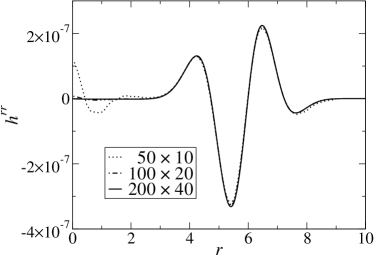
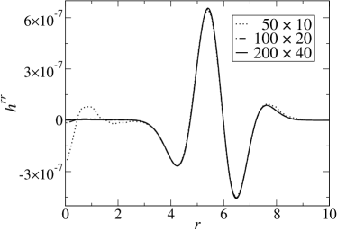
Figure 1: Radial profile of $h^{rr}$ at $t=6$ at the equator (upper panel) and at the pole (lower panel). Three different resolutions $n_{r}\times n_{\theta}$ are shown: $50\times 10$ (dotted lines), $100\times 20$ (dot-dashed lines) and $200\times 40$ (solid lines).

We display in Fig. 1 the radial profile of the component $h^{rr}$ at the end of the simulation, $t=6$, for three different numerical resolutions $n_{r}\times n_{\theta}$. Since the amplitude of the wave is sufficiently small to be considered a linear perturbation, we can compare the numerical solution with the analytical expression for the Teukolsky wave at each time. The solution agrees in the propagation speed of the wave, its amplitude and the asymptotic decay with increasing radius with the analytical solution. The Sommerfeld condition at the outer boundary produces ingoing reflections with at most an amplitude square of the outgoing wave, as it is prescribed by the imposed condition. In Fig. 2 we plot the absolute errors of the numerical solution with respect to the analytical values of all the non zero components of the tensor $h^{ij}$ at $(t,r,\theta)=(6,0,\pi/2)$ (Fig. 1 shows that the maximum of the absolute error appears at $r=0$), for different resolutions. We obtain an order of convergence of $3.4$, $3.6$, $3.8$, and $4.6$ for the components $h^{rr}$, $h^{\theta\theta}$, $h^{\varphi\varphi}$ and $h^{r\theta}$, respectively, which is close to the fourth-order of the corresponding Runge-Kutta method. Note that, since the background has $\beta^{i}=0$, the source term $S_{w2}=0$ in Eq. (29); in this case we observe no significant reduction of the convergence order.

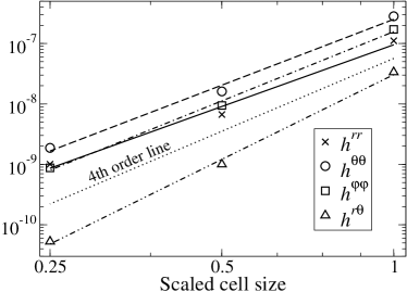
Figure 2: Absolute errors of the numerical solutions with respect to the analytical values of all the non zero components of the tensor $h^{ij}$ at $(t,r,\theta)=(6,0,\pi/2)$ in terms of the (scaled) cell size. Solid, dashed, dot-dashed and dot-dot-dashed lines fit the errors for the component $h^{rr}$, $h^{\theta\theta}$, $h^{\varphi\varphi}$ and $h^{r\theta}$, respectively. Dotted line is the reference of fourth-order of convergence.

V Evolution of equilibrium rotating neutron stars

To test the performance of the passive FCF formulation in an astrophysical scenario we perform simulations of the evolution of isolated neutron stars. In this case the gravitational field is sufficiently strong to need to go beyond the Newtonian limit and at the same time the GW back-reaction is sufficiently small for the passive FCF approximation to be valid. Table 1 summarizes the approximations made in the simulations of this section.

V.1 Initial model and grid

We construct the initial data using the numerical code rotstar_dirac of the lorene library Lorene , which computes axisymmetric and uniformly rotating neutron stars in equilibrium in the FCF formalism lapming06 . We use a polytropic equation of state, $P=K\rho^{\Gamma}$, with $\Gamma=2$ and $K=100$ (in $c=G=M_{\odot}=1$ units), to construct a neutron star with a 550 Hz rotation frequency, an ADM mass $M_{\rm ADM}=1.4874\,M_{\odot}$ and a radius $R=15.18$ km. The surface is located at a coordinate radius $r_{*}=12.86$ km at the equator. The wavelegth of GWs at the frequency of the fundamental f-mode ($1.65$ kHz as measured from our numerical simulations of Sec. V.3) is $\lambda_{\rm F}=181$ km. Following Thorne80 the (local) wave zone for our neutron star model is located at $r>>\lambdabar\equiv\lambda/(2\pi)=28.8$ km.

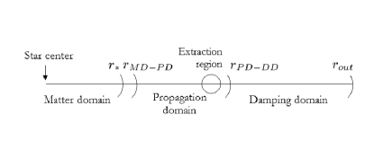
Figure 3: Scheme of the radial grid used in the code for rotating neutron star simulations.

Thanks to the use of spherical coordinates, we can adapt the radial grid to cover different domains of the space with the resolution needed on each domain. In the case of a neutron star we have different resolution requirements inside the neutron star, where hydrodynamic variables have to be properly resolved, and outside, where it is sufficient to resolve the wavelength of the outgoing GWs.

	regular resolution	high resolution
$r_{\rm MD-PD}/r_{*}$	1.19	1.19
$r_{\rm PD-DD}/\lambdabar_{\rm F}$	10.5	10.5
$r_{\rm out}/\lambdabar_{\rm F}$	104.2	104.2
$\Delta r_{\rm PD-DD}/\lambda_{\rm F}$	5	10
$n_{r,{\rm MD}}$	80	160
$n_{r,{\rm PD}}$	346	690
$n_{r,{\rm DD}}$	43	88
$n_{r}$	469	938
$n_{\theta}$	16	32

Table 2: Parameters used in the finite differences grid in simulations of neutron star evolution.

For the finite difference grid, we consider three radial domains covering the computational domain (see Fig. 3): the matter domain (MD) contains the neutron star, extends from the center to a radius $r_{\rm MD-PD}$ slightly larger than the stellar radius $r_{*}$. This domain is covered by an equidistant radial grid. The propagation domain (PD), extends from $r_{\rm MD-PD}$ to a radius $r_{\rm PD-DD}>>\lambdabar$. In this region the radial grid spacing increases geometrically outwards, such that the GWs are well resolved. Near the outer edge of the domain, the GWs reach the wave zone, and hence it is an appropriate radius to perform the GW extraction. The damping domain (DD) extends from $r_{\rm PD-DD}$ to the outer boundary of the numerical grid $r_{\rm out}$. We locate the outer boundary such that an outgoing wave generated at the center at $t=0$ and traveling at the speed of light reaches the outer boundary at the end of the simulation. This configuration minimizes the effect of spurious numerical artifacts at the outer boundary which where found in our preliminary work CC10 . In the damping domain the radial grid spacing increases geometrically outwards and the wavelength of the GWs is not well resolved. This produces an effective damping of the outgoing GWs which helps to reduce the effect of the outer boundary conditions. To construct the finite difference grid we need to provide the values of $r_{\rm MD-PD}$, $r_{\rm PD-DD}$, $r_{\rm out}$, the number of grid points inside of the MD, the grid spacing $\Delta r_{\rm PD-DD}$ at $r_{\rm PD-DD}$ (which automatically fixes the number of points inside PD), and the cell radial spacing ratio between consecutive ones at DD (which fixes the number of points in this domain). We perform simulations with two resolutions, labeled regular and high, whose grid parameters are given in table 2.

For the spectral grid we use two resolutions labeled regular and high. The regular resolution grid consists of $5$ radial spectral domains covering the finite difference grid, $4$ domains with $33$ and $1$ with $17$ radial collocation points, and a compactified spectral domain from $r_{\rm out}$ to infinity with $17$ collocation points. The $\theta$ direction is covered by $5$ collocation points. The high resolution grid consist of $13$ spectral domains, $6$ domains with $33$ and $7$ with $17$ collocation points, and a compactified domain with $17$ collocation points. The $\theta$ direction is covered by $17$ collocation points.

V.2 Equilibrium neutron stars

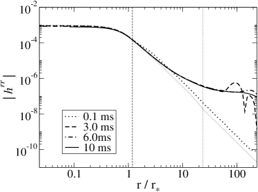
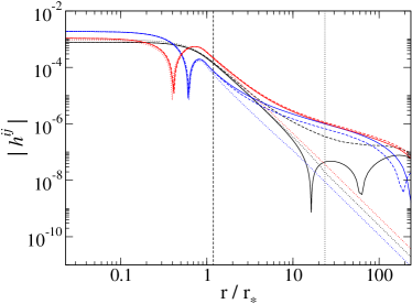
Figure 4: Radial profiles of $h^{ij}$ for numerical simulations of neutron stars. The upper panel shows four snapshots of the evolution of $h^{rr}$ and the initial stationary solution (grey line). The lower panel shows the components $h^{rr}$ (black lines), $h^{\theta\theta}$ (blue lines), and $h^{\varphi\varphi}$ (red lines) for the initial stationary configuration (dotted lines), and the final configuration at $10$ ms (dashed lines for the regular and solid lines for the high resolution spectral grid).

Before attempting to solve the full coupled evolution of spacetime and hydrodynamics in neutron stars, we perform simulations in a more simplified setting. We evolve the hyperbolic sector of the passive FCF formalism in a fixed non-trivial background (non-vanishing $N$, $\beta^{i}$, $\psi$ and hydrodynamic variables) corresponding to the equilibrium configuration of a rotating neutron star. Therefore, we evolve stationary initial data for the variable vector ${\bf W}$ and keep the variable vector ${\bf U}$ and ${\bf V}$ fixed during the evolution of ${\bf W}$.

Our fiducial model has regular resolution concerning both the finite difference grid and the spectral one. The background model is computed with FCF gravity, but we recompute the elliptic part, ${\bf V}$, at the beginning with the CFC approximation, i.e., the background is evolved in the same way as it is in the simulations of the next section, where the vector ${\bf V}$ is also evolved in time. The consequences of this modification on the background metric are evaluated below. We evolve the system of equations for the vector ${\bf W}$ for $10$ ms. Due to small numerical discrepancies between the initial data for ${\bf W}$ and the numerical stationary solution of the equations a perturbation in the vector ${\bf W}$ appears and propagates outwards. The upper panel of Fig. 4 shows four snapshots of the evolution of the $h^{rr}$ component compared to the stationary solution (grey line). Note that the perturbation reaches the outer boundary at about $3$ ms, well before the end of the simulation. This is due to the unphysical superluminical propagation of the wave in the damping domain, where its wavelength is unresolved. However, due to the smallness of $h^{ij}$ at the outer boundary, about $3$ orders of magnitude smaller than at the center, spurious reflections are not noticeable in the simulations. At the end of the simulation the outgoing wave leaves the numerical domain and an equilibrium configuration remains. We can compare this solution with the initial stationary data to look for numerical discrepancies. At the center the initial configuration is recovered within $\sim 10\%$ accuracy. For distances $r/r_{*}\geq 10$ (see upper panel of Fig. 4) there are larger deviations, and the components of $h^{ij}$ decay approximately as $r^{-1}$ instead of $r^{-3}$ as in the initial stationary model. Since GWs are contained in the part of $h^{ij}$ decaying as $r^{-1}$, the erroneous decay observed in the simulations at large distances will lead to a constant offset in the computed GW amplitude. This offset can be comparable to the amplitude of GWs produced by small perturbations (see CC10 for more details). We discuss the possible causes for this behavior below.

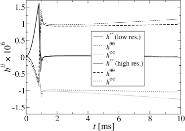
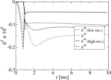
Figure 5: Time evolution of $h^{ij}$ at $r/r_{*}=19.44$ and $\theta=\pi/2$. Left (right) panel shows the diagonal (non-diagonal) components. We plot two different finite differences resolutions: regular (thin lines) and high (thick lines).

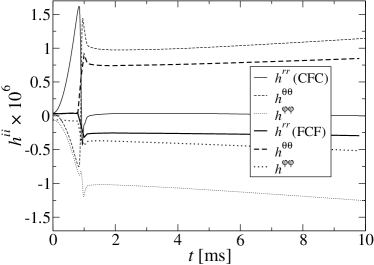
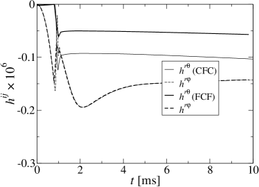
Figure 6: Same as Fig. 5, but we compare simulations using the CFC approximation (thin lines) and the full FCF metric (thick line) for the background metric V.

One important reason for the appearance of offsets is the accuracy of the numerical solution of the elliptic equations. We have performed simulations increasing the spectral grid resolution, but keeping the same regular resolution for the finite difference grid. The spectral grid resolution affects the accuracy of the computation of the background ${\bf V}$ computed at the beginning of the simulation. The lower panel of Fig. 4 shows the final configuration of the diagonal components of $h^{ij}$ for the regular and high resolution spectral grid, compared to the initial equilibrium configuration. The error at the center of the equilibrium configuration at the end of the simulation does not improve with respect to the regular resolution spectral grid. The erroneous decay of $h^{ij}$ improves significantly for the $h^{rr}$ component, and we recover the correct $r^{-3}$ decay in the whole propagation domain. However, the $h^{\theta\theta}$ and $h^{\varphi\varphi}$ components do not improve significantly. Therefore, there is a strong sensitivity of the $h^{rr}$ component on the spectral metric resolution, and hence on the accuracy of the computation of ${\bf V}$, because the variables in ${\bf V}$ appear in the leading terms of the equations for ${\bf W}$, Eqs. (9)–(11). However, spectral resolution does not seem to cure the problems in $h^{\theta\theta}$ and $h^{\varphi\varphi}$ which, as we show below, are related to other sources of inaccuracy in the solution of ${\bf V}$. Because of the better performance of the high resolution spectral metric we use this resolution for all simulations hereafter.

To check the effect of the finite difference grid resolution we have performed simulations with the high resolution grid, keeping the high resolution spectral grid fixed. The finite difference grid resolution affects the accuracy of the solution of the vector ${\bf W}$, i.e. the evolution of $h^{ij}$. In Fig. 5 we plot the time evolution of the components of the tensor $h^{ij}$ (left panel for the diagonal components and right panel for non-diagonal components) at $r/r_{*}=19.44$, for the two finite difference grid resolutions. This coordinate radius is close to the outer boundary of the propagation domain and the inner edge of the extraction region for GWs (see next section). About $1$ ms after the beginning of the simulation, the outgoing wave reaches this radius visible in Fig. 5 as a sudden rise of all components of $h^{ij}$. After the outgoing wave leaves the numerical domain the value of $h^{ij}$ does not settle down to the initial equilibrium value, but to an offset value, decaying as $r^{-1}$. All components converge with finite difference grid resolution to an offset value. The offset of the component $h^{rr}$ cannot be appreciated in Fig. 5 since it is much smaller than in the other components.

Apart from the numerical error in the computation of ${\bf V}$ due to a finite spectral grid resolution, the approximating of the vector ${\bf V}$ by the solution of the CFC equations instead of the full FCF elliptic equations might also introduce small errors in the vector ${\bf V}$, which are sufficiently large to explain the observed offsets. Although we still cannot solve the FCF elliptic equations with CoCoNuT in a simulation with spacetime evolution, for the case of fixed vectors $\bf U$ and $\bf V$ considered in this section, we can take the full FCF solution for $\bf V$ computed by the initial data solver rotstar_dirac. We have performed simulations with the regular and high resolution finite difference grids and the FCF background metric vector $\bf V$. The resolution used for the spectral solver in the initial data generator, rotstar_dirac, fixes the numerical accuracy of the vector ${\bf U}$. Unfortunately, due to internal code limits of rotstar_dirac, the maximum resolution that we could achieve was $8$ radial domains, $5$ with $33$ and $3$ with $17$ collocation points, and $17$ collocation points in the $\theta$ direction. This resolution lays in between the regular and the high resolution spectral grids used for CFC metric computations. Fig. 6 compares the evolution of $h^{ij}$ close to the GW extraction radius, $r/r_{*}=19.44$, with the CFC and the FCF background. The offset in $h^{\theta\theta}$, $h^{\varphi\varphi}$ and $h^{r\theta}$ is reduced when the CFC approximation is removed and the background is computed with the full general relativistic FCF formulation. The offset in $h^{rr}$ increases, however, although this is expected since the resolution of the spectral grid is lower in the FCF case than in the CFC case. We observe no change in the offset of the $h^{r\varphi}$ component.

We conclude that the main reason for the offset in $h^{ij}$ at large distance from the source is the accuracy of the computation of the vector ${\bf V}$. Both the resolution of the spectral grid and the neglected terms in the elliptic part due to the passive FCF approximation are responsible for this loss of accuracy, affecting in each case different components of $h^{ij}$. This defines the spectral grid resolution necessary for the simulations in the next section, but the use of the passive FCF approximation still introduces an offset which cannot be removed. The resolution tests show that the finite difference grid is adequate to evolve ${\bf W}$, and is not responsible for the offset.

The order of convergence of the code is difficult to evaluate due to the fact that if we increase the finite difference grid resolution the solution converges towards an offset solution and not to the equilibrium one, and at the same time this offset converges with the spectral grid resolution and is affected by the passive FCF approximation. However, we can check the time behavior of the stationary solutions after the outgoing wave is gone. In Fig. 5 the time evolution of all $h^{ij}$-components suffers a time-drift which is due to numerical diffusion. We fit the evolution of the $h^{\theta\theta}$-component between $t_{1}=4$ ms and $t_{2}=10$ ms to $h^{\theta\theta}(t_{1})+C\cdot(t_{2}-t_{1})^{p}$. The fitted value for the power $p$ is $1.7$ and $1.8$ for the regular and high resolution simulations, respectively. If we consider that $C\sim{\Delta r}^{p}$, we can also compute the power as $p=log(C_{\rm regular}/C_{\rm high})/log{\,2}$, which is $1.96$. Therefore, the order of convergence is close to second-order, due to the mixture of implicit and explicit terms in the fourth-order Runge-Kutta scheme. If we apply this analysis to other components of $h^{ij}$, we find a similar order of convergence.

V.3 Perturbed equilibrium configuration of rotating neutron star

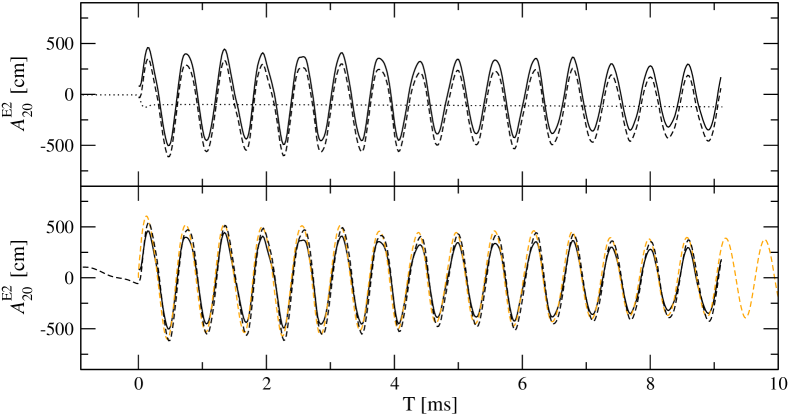
Figure 7: Quadrupolar component of the GW extracted from simulations of an oscillating neutron star. The upper panel shows the extrapolated waveform at infinity (black dashed line) and the offset-corrected waveform extrapolated at infinity (black solid line). The offset is corrected using the average value of the waveform of a non-perturbed neutron star simulation (black dotted line). The lower panel shows the offset-corrected waveform at an extraction radius of $r/r_{*}=19.44$ (black dashed line) and extrapolated at infinity (black solid line), compared to the quadrupole formula (orange dashed line).

The last test consists in the evolution of an oscillating neutron star with coupled hydrodynamics and spacetime evolution, i.e. we evolve the coupled system for ${\bf U}$, ${\bf V}$ and ${\bf W}$ in the passive FCF approximation. We use the regular resolution finite difference grid and the high resolution spectral grid. We initiate the oscillations by adding a small $l=2$ velocity perturbation (about $1\%$ of the speed of light) to the stationary initial data used in the previous subsection. Previous preliminary studies CC10 show that the gravitational radiation has to be extracted close to $r_{\rm PD-DD}$ but still inside the propagation domain, where the wavelength of the fundamental mode is resolved by about 5 grid points in the regular resolution finite difference grid.

For asymptotically flat spacetimes, as the one used in our simulations, and since the Dirac gauge tends to the TT gauge far from the strong field region Smarr78 , it is possible to compute the amplitude of the plus polarization of the GW, i.e. the real part of the $\Psi_{4}$ Weyl scalar, detected by an observer at a distance $R$ with an observation angle $\Theta$ with respect to the rotation axis as

$$h_{+}(R,\Theta,T)=\lim_{R\to\infty}\frac{h^{\varphi\varphi}(R,\Theta,T)-h^{\theta\theta}(R,\Theta,T)}{2}.$$ (32)

In axisymmetry, the cross polarization, $h_{\times}$, vanishes. In general, one should compute outgoing null geodesics for each angle $\theta$ and determine the observation angle $\Theta$ and the distance $R$, and then use the numerical value of $h^{ij}$ at the extraction radius to determine $h_{+}(R,\Theta,T)$. Thanks to the equatorial symmetry, the curves $\theta=\pi/2$ on $\Sigma_{t}$ are null geodesics, and will be observed at a distance $R$ with inclination angle $\Theta=\pi/2$. The distance to an observer located at a coordinate radius $r$ can be easily computed as

$$R(r)=\int_{0}^{r}\sqrt{\gamma_{rr}(r,\theta=\pi/2)}\,dr\approx\int_{0}^{r}\psi(r,\theta=\pi/2)^{2}\,dr.$$ (33)

For our neutron star model, the spacetime surrounding it is not extremely curved, and radial null geodesics at other angles are approximately curves with constant $\theta$, i.e. $\Theta\approx\theta$. If we integrate the distance $R$ as in Eq. (33) at different angles $\theta$, the difference between equator and polar axis is about $0.04\%$. Hence, for neutron stars we can safely compute $h_{+}$ at any angle using the numerical value of $h^{ij}$ at the extraction radius $r_{\rm ext}$ as

$$h_{+}(R,\theta,T)\approx\frac{h^{\varphi\varphi}(r_{\rm ext},\theta,t)-h^{\theta\theta}(r_{\rm ext},\theta,t)}{2}\frac{R(r_{\rm ext})}{R},$$ (34)

where $T\equiv t-R/c$ is the retarded time. Note that Eq. (34) is approximate and valid only in the wave zone, i.e. for $r_{\rm ext}>>\lambdabar_{\rm F}$.

In axisymmetry and with equatorial symmetry, the multipolar decomposition of the radiation field is Thorne80 :

$$h_{+}(R,\theta,T)=\frac{1}{R}\left(A^{E2}_{20}(T)T^{E2,20}(\theta)+A^{E2}_{40}T^{E2,40}(\theta)+...\right)$$ (35)

We have extracted the amplitude of the $l=2$ and $4$ multipoles, $A^{E2}_{20}$ and $A^{E2}_{40}$, respectively, from the numerically computed $h_{+}$, at all radial points between $15r_{*}$ and $19.44r_{*}$. For post-Newtonian sources, as in our case, we expect the amplitude of the multipoles to decrease with $l$ Thorne80 . We were unable to extract higher-order multipoles because of the smallness of the signal, which made the numerical extraction too noisy. Since the extraction radii are relatively close to the source, in the interval $6.7\lambdabar$-$8.7\lambdabar$, there is a small radial dependence of the GW amplitude and phase on the extraction radius. This dependence corresponds to $r^{-p}$, $p\geq 2$, components in $h^{ij}$, where the leading term is $r^{-2}$ and can be fitted to extract the waveform at infinity using a procedure similar to Baiotti09 . To extrapolate both phase and amplitude, we proceed in two steps:
i) First, we perform a least squares fit of the retarded time of each maxima in the waveform as a function of the extraction radius $R$ to

$$T_{\rm max}(R)=T_{\rm max}(\infty)+\frac{C}{R}.$$ (36)

We use the average value of $C$ for all maxima, $<C>/r_{*}=0.2245$ ms, to correct the phase of the waveform as

$$T(\infty)=T(R)-\frac{<C>}{R}.$$ (37)

ii) Once the phase is corrected, we fit the amplitude of the waveform at constant $T(\infty)$ as a function of $R$ to

$$A^{E2}_{20}(R,T(\infty))=A^{E2}_{20}(\infty,T(\infty))+\frac{C^{\prime}}{R}.$$ (38)

The resulting fitted value of $A^{E2}_{20}(\infty,T(\infty))$ is the waveform extrapolated at infinity. To estimate the finite distance effects we present results of the waveform extracted at a finite distance $r_{\rm ext}=19.44r_{*}$ and extrapolated at infinity.

An alternative approach to compute the GW amplitude is to use the post-Newtonian wave-generation formalism. This is possible if the sources allow for a post-Newtonian expansion, i.e. $(v/c)^{2}\sim M/r_{*}<1$. For slow-motion sources Thorne80 , for which $r_{*}<<\lambdabar$, it is possible to write the amplitudes of the different multipoles as volume integrals over the matter sources. Truncating the integrals at the lower post-Newtonian level, i.e. with Newtonian sources, the quadrupolar component results in the well known quadrupole formula Einstein18 . In axisymmetry the quadrupole formula reads

$$A^{E2}_{20}=8\sqrt{\frac{\pi}{15}}\frac{d^{2}}{dt^{2}}\left\{\int D\,(3z^{2}-1)\,r^{2}\sqrt{\gamma}\,drd\theta d\varphi)\right\},$$ (39)

with $z\equiv\cos{\theta}$. Using the continuity equation, $J^{\mu}_{;\mu}=0$, one of the time derivatives can be removed analytically (cf. Blanchet90 ),

$$A^{E2}_{20}=8\sqrt{\frac{\pi}{15}}\frac{d}{dt}\Bigg{\{} \int D\,\Big{(}v^{*r}(3z^{2}-1)$$ (40)

$$-3v^{*\theta}z\sqrt{1-z^{2}}\,\,\Big{)}\,r\sqrt{\gamma}\,drd\theta d\varphi)\Bigg{\}},$$

where $v^{*i}\equiv\alpha v^{i}-\beta^{i}$. The latter formula is more convenient from the numerical point of view, since only one time derivative has to be evaluated numerically. We use it in this work.

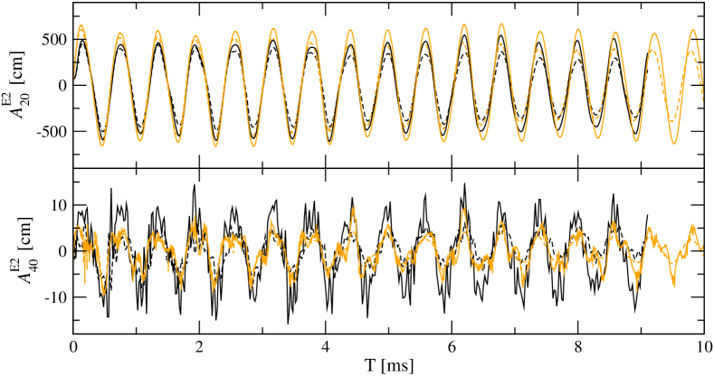
Figure 8: GW extracted from simulations of an oscillating neutron star. Upper and lower panels show the quadrupolar and hexadecapolar component respectively. On each panel we compare simulations for regular (dashed lines) and high (solid lines) resolution finite differences grid. The offset-corrected and waveform extrapolated at infinity computed with the direct extraction method (black lines) is compared to the PN method (quadrupole and hexadecapole formulae, orange lines).

In equatorial symmetry, the hexadecapolar component is Moenchmeyer91 ; Faye03 :

$$A^{E2}_{40}=\frac{\sqrt{5\pi}}{126}\frac{d^{4}}{dt^{4}}\left\{\int D\,\left(7z^{4}-6z^{2}+\frac{3}{5}\right)\,r^{4}\sqrt{\gamma}\,drd\theta d\varphi)\right\}.$$ (41)

In a similar way as for the quadrupole formula, it is possible to remove one time derivative using the continuity equation (cf. Moenchmeyer91 ; Faye03 ):

$$A^{E2}_{40}= \frac{2\sqrt{5\pi}}{63}\frac{d^{3}}{dt^{3}}\Bigg{\{}\int D\,\Bigg{[}v^{*r}\left(7z^{4}-6z^{2}+\frac{3}{5}\right)$$ (42)

$$+v^{*\theta}\left((3-7z^{2})z\sqrt{1-z^{2}}\right)\Bigg{]}\,r^{3}\sqrt{\gamma}\,drd\theta d\varphi)\Bigg{\}}.$$

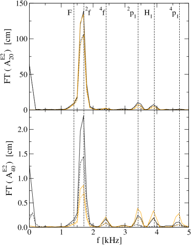
Figure 9: Fourier transform of the GW amplitude of an oscillating neutron star. Upper and lower panels show the quadrupolar and hexadecapolar component respectively. On each panel we compare simulations for regular (dashed lines) and high (solid lines) resolution finite differences grid. The Fourier transform of the offset-corrected waveform computed with the direct extraction method (black lines) is compared to the quadrupole formula (orange lines).

In the upper panel in Fig. 7, we plot the time evolution of the quadrupolar component $A^{E2}_{20}$ computed with Eq. (34) (direct extraction hereafter) extrapolated at infinity. The waveform clearly shows a constant offset which is unphysical. The dotted line shows the GW corresponding to the model in the previous section with the same resolution, but fixed ${\bf U}$ and ${\bf V}$, and no initial perturbation. In this case we do not observe any oscillation, since the star itself is not oscillating, but an offset appears of similar magnitude as in the oscillating case. We can use the value of the offset at each time from the non-perturbed simulation to remove the offset in the oscillating simulation by simple subtraction of both GW signals.

In the lower panel of Fig. 7 we compare the offset corrected waveform to the result of the quadrupole formula. There is a remarkable good agreement in the frequency and phase. The Fourier transform of the waveform is shown in the upper panel of Fig. 9. Within the numerical frequency resolution of the Fourier transform of the waveform, about $0.02$ kHz, we do not observe differences in the frequency between the direct extraction method and the quadrupole formula. That sets an upper limit of $1\%$ for the frequency difference in the fundamental oscillation mode, $f_{\rm F}=1.66$ kHz. The phase difference between both GW extraction methods, estimated as the relative difference in the retarded time at the maxima, is smaller than $1\%$. The corrected signal (solid line in Fig. 7) agrees with the quadrupole formula within $30\%$. Therefore, the only big discrepancy with the quadrupole formula is due to the error committed in the computation of the vector ${\bf V}$, using the passive FCF approximation and the spectral grid resolution. The quadrupole formula is an approximate formula, which is valid in the slow-motion post-Newtonian limit. The error in the formula should be of the order $(v/c)^{2}\sim M/r_{*}$, which for our system is $\sim 17\%$. Therefore, the $30\%$ discrepancy in the amplitude is compatible with the approximation error of the quadrupole formula. Note that the waveform extracted at finite distance suffers from additional errors. For example, at $19.44r_{*}$ (black dashed line in Fig. 7) the amplitude of the waveform differs about $30\%$ from the extrapolated waveform at infinity and its phase about $5\%$.

In the case of the hexadecapolar component $A^{E2}_{40}$ (lower panel of Figs. 8 and 9), the direct extraction method shows an important contribution due to numerical noise. Note that the hexadecapolar component is about a $2\%$ contribution to the total waveform $h_{+}$. Therefore, this numerical noise appears because of errors in the evolution of $h^{ij}$ below $1\%$, which are expected in our simulations. In this case the hexadecapole formula provides a good estimate of the phase and the frequency ($\sim 5\%$), however, the error in the amplitude is about $50\%$. Note that for the hexadecapolar component there are possible sources of error in both the direct extraction method, due to the smallness of the amplitude, and in the hexadecapole formula, due to the three numerical time derivatives that we have to perform. Therefore, it is difficult to disentangle which one is a better approximation to the waveform. Nevertheless, both methods provide a reasonable agreement, and we are confident that the amplitude computed with any of the two methods is a rather good order-of-magnitude estimate of the hexadecapolar component.

To test the effect of the finite difference grid resolution, we compare simulations with regular and high resolution, and the same high spectral metric resolution. Fig. 8 shows the offset-corrected values of $A^{E2}_{20}$ and $A^{E2}_{40}$ for both resolutions. For the offset correction we use the corresponding regular and high resolution simulations of the previous section. We compare with the post-Newtonian wave generation formalism (quadrupole and hexadecapole formulae, PN method for short) for both resolutions. In both methods, direct extraction and PN method, we observe a damping of the waveforms which is reduced when increasing the resolution. The PN method only uses information in the GW generation zone ($r<r_{*}$), contrary to the direct extraction method, where the wave is propagated from the generation zone to the wave zone. However, in both cases the damping observed in the waveforms is of similar magnitude. That means that the source of the damping must be caused by numerical inaccuracies in the region close to the star, but not in the propagation domain. In other words, we observe a numerical damping of the oscillations of the star itself, but not of the waves during their propagation towards the GW extraction point.

VI Summary and conclusions

We have reviewed the fully constrained formalism, which is a natural generalization of the CFC approximation of GR, and we have expressed the system of FCF equations in a form suitable for numerical simulations. We have presented a numerical scheme to solve the FCF system using spectral methods for the elliptic part and finite difference schemes for the hyperbolic part. In the simulations presented here we have neglected the back-reaction of the GWs onto the dynamics, which we call passive FCF. This work focuses on the stability and convergence of the hyperbolic part of the FCF equations, since the stability issues of the elliptic part were considered by CC09 . We have presented a fourth-order finite difference scheme to solve the system of hyperbolic equations that makes use of implicit relations, to provide the necessary stability of the algorithm. We have solved the equations in spherical coordinates and axisymmetry.

We have performed convergence tests for the hyperbolic part, in which the gravitational radiation of the system is encoded, using a simple vacuum test with known analytical solution: the Teukolsky waves. We have shown the stability and convergence of the numerical evolution which is consistent with the fourth-order convergence of the numerical scheme. We have performed the evolution of equilibrium neutron stars and checked that the numerical code is able to maintain such configurations in equilibrium keeping the hyperbolic part to an accuracy of second-order. We interpret the drop to second-order convergence in all our simulations with matter content as an inconsistency in our numerical scheme in this regime, due to the mixture of explicit and implicit terms in the Runge-Kutta scheme. In order to improve the order of convergence one should use IMEX methods to solve the system of equations AsRuuSpi ; PaRu . Although this approach is beyond the scope of this work, it may be considered in the future.

Finally, we have performed simulations of the evolution of an oscillating equilibrium neutron star. We have extracted the GW signature from the metric components in the wave zone. We have compared the results from the direct extraction method with calculations using the post-Newtonian wave generation formalism, namely the Newtonian quadrupole and hexadecapole formulae. We found that the approximate quadrupole formula describes within $\sim 30\%$ error the quadrupolar component of the wave. This is consistent with its nominal post-Newtonian error ($\sim 20\%$). Similar good agreement of the quadrupole formula with BSSN simulations was found by Shibata03 ; Reisswig11 . We were able to extract the hexadecapole component of the wave, although numerical noise is considerably larger than in the quadrupole component. The comparison with the Newtonian hexadecapole formula agrees in frequency, phase and order of magnitude, however the comparison is limited by the numerical accuracy of both wave extraction methods. We found that the evolution of the hyperbolic part of the metric is very sensitive to inaccuracies in the elliptic sector, resulting in offsets in the GW signature. The main sources for inaccuracies are the number of collocation points in the spectral solver for the elliptic part and the absence of back-reaction terms. We were able to get convergent results increasing the spectral resolution, however, an offset still remained due to the passive FCF approximation. We conclude that GWs back-reaction should be included in the future, as well as an improvement in the accuracy of the numerical solution of the elliptic equations, in order to remove these offsets.

We note that all simulations that we have performed in this work make use of spherical orthonormal coordinate grids, for the whole computation domain, in axisymmetry. Our simulations are among the few multidimensional simulations of Einstein equations in spherical coordinates. In the context of 3+1 formulations, some of the first simulations of black hole formation used spherical coordinates Stark85 ; Evans86 , however the formulations used in those works were unstable leading to exponentially growing constraint violations. Although some work has been done to reformulate the BSSN equations in order to ease its evolution in spherical coordinates Brown05 ; Alcubierre05 ; Alcubierre11 , these reformulations have been only tested for 1D numerical problems. The use of multi-block methods in BSSN simulations Tiglio05 ; Pollney11 allows to make use of spherical wavezone grids to take advantage of topologically adapted grids, but they keep a cartesian grid in the central region. On the other hand, spherical coordinates are widely used in the null formulations (see WinicourLR ), mostly in the context of Cauchy-characteristic matching and extraction (e.g. Reisswig09 ; Babiuc11 ; Reisswig11 ), although stand-alone characteristic formulations have still very few numerical applications (e.g. Gomez98 ; Siebel02 ).

We think that the reason for the success of our simulations in spherical coordinates is twofold. First, we use an implicit-explicit algorithm to solve the system of hyperbolic equations, whereas we solve implicitly the terms in the equations leading to instabilities. Second, only two degrees of freedom of the system, the GWs, are evolved by means of hyperbolic equations, while the rest are the result of the computation of elliptic equations. This main feature of FCF is possibly crucial to provide the extra stability to the numerical algorithm. We are not sure, whether both requirements are indeed necessary to perform stable simulations in spherical coordinates, or whether the implicit-explicit scheme gives rise to the stability of the numerical algorithm. It would be interesting to explore the behavior of purely hyperbolic formulations with our implicit-explicit algorithm in spherical coordinates.

Appendix A Runge-Kutta schemes and partially implicit evaluation of the $S_{w2}$ term

In this appendix we describe with more details the numerical method used in the evolution of the variables $\bf W$, which has a partially implicit evaluation of the $S_{w2}$ term in the evolution of the $w^{ij}_{k}$ tensor. They are based in the explicit Runge-Kutta schemes of second, third and fourth-order. We show the procedure with the second and third-order ones.

The optimal second and third-order Runge-Kutta schemes ShuOsher of a general evolution equation in time $t$ for the variable $u$ of the form $u_{t}=L(u)$ are respectively

$$u^{(1)} = u^{n}+\Delta t\,L(u^{n}),$$

$$u^{n+1} = \frac{1}{2}\left(u^{n}+u^{(1)}+\Delta t\,L(u^{(1)})\right),$$ (43)

and

$$u^{(1)} = u^{n}+\Delta t\,L(u^{n}),$$

$$u^{(2)} = \frac{3}{4}u^{n}+\frac{1}{4}u^{(1)}+\frac{1}{4}\Delta t\,L(u^{(1)}),$$

$$u^{n+1} = \frac{1}{3}u^{n}+\frac{2}{3}u^{(2)}+\frac{2}{3}\Delta t\,L(u^{(2)}),$$ (44)

where $u^{n}=u(t^{n})$ and $u^{n+1}$ is the numerical approximation for the value $u(t^{n}+\Delta t)$.

The corresponding methods used in order to evolve $\bf W$ based on the previous Runge-Kutta schemes are:

1. Based on the second-order Runge-Kutta scheme:

   $$h^{ij(1)} = h^{ij(n)}+\Delta t\,S_{h}(h^{ij(n)},\hat{A}^{ij(n)},w^{ij(n)}_{k},{\bf V}^{(n)}),$$

   $$\hat{A}^{ij(1)} = \hat{A}^{ij(n)}+\Delta t\,S_{\hat{A}}(h^{ij(n)},\hat{A}^{ij(n)},w^{ij(n)}_{k},{\bf U}^{(n)},{\bf V}^{(n)}),$$

   $$w^{ij(1)}_{k} = w^{ij(n)}_{k}+\Delta t\,S_{w1}(h^{ij(1)},\hat{A}^{ij(1)},{\bf V}^{(n)})$$

   $$+ \Delta t\,S_{w2}(w^{ij(n)}_{k},{\bf V}^{(n)}),$$

   $$h^{ij(n+1)} = \frac{1}{2}h^{ij(n)}+\frac{1}{2}h^{ij(1)}+\frac{1}{2}\Delta t\,S_{h}(h^{ij(1)},\hat{A}^{ij(1)},w^{ij(1)}_{k},{\bf V}^{(n)}),$$

   $$\hat{A}^{ij(n+1)} = \frac{1}{2}\hat{A}^{ij(n)}+\frac{1}{2}\hat{A}^{ij(1)}$$

   $$+ \frac{1}{2}\Delta t\,S_{\hat{A}}(h^{ij(1)},\hat{A}^{ij(1)},w^{ij(1)}_{k},{\bf U}^{(n)},{\bf V}^{(n)}),$$

   $$w^{ij(n+1)}_{k} = \frac{1}{2}w^{ij(n)}_{k}+\frac{1}{2}w^{ij(1)}_{k}+\frac{1}{2}\Delta t\,S_{w1}(h^{ij(n+1)},\hat{A}^{ij(n+1)},{\bf V}^{(n)})$$ (45)

   $$+ \frac{1}{2}\Delta t\,S_{w2}(w^{ij(1)}_{k},{\bf V}^{(n)}).$$

2. Based on the third-order Runge-Kutta scheme:

   $$h^{ij(1)} = h^{ij(n)}+\Delta t\,S_{h}(h^{ij(n)},\hat{A}^{ij(n)},w^{ij(n)}_{k},{\bf V}^{(n)}),$$

   $$\hat{A}^{ij(1)} = \hat{A}^{ij(n)}+\Delta t\,S_{\hat{A}}(h^{ij(n)},\hat{A}^{ij(n)},w^{ij(n)}_{k},{\bf U}^{(n)},{\bf V}^{(n)}),$$

   $$w^{ij(1)}_{k} = w^{ij(n)}_{k}+\Delta t\,S_{w1}(h^{ij(1)},\hat{A}^{ij(1)},{\bf V}^{(n)})$$

   $$+ \Delta t\,S_{w2}(w^{ij(n)}_{k},{\bf V}^{(n)}),$$

   $$h^{ij(2)} = \frac{3}{4}h^{ij(n)}+\frac{1}{4}h^{ij(1)}+\frac{1}{4}\Delta t\,S_{h}(h^{ij(1)},\hat{A}^{ij(1)},w^{ij(1)}_{k},{\bf V}^{(n)}),$$

   $$\hat{A}^{ij(2)} = \frac{3}{4}\hat{A}^{ij(n)}+\frac{1}{4}\hat{A}^{ij(1)}+\frac{1}{4}S_{\hat{A}}(h^{ij(1)},\hat{A}^{ij(1)},w^{ij(1)}_{k},{\bf U}^{(n)},{\bf V}^{(n)}),$$

   $$w^{ij(2)}_{k} = \frac{3}{4}w^{ij(n)}_{k}+\frac{1}{4}w^{ij(1)}_{k}+\frac{1}{4}\Delta t\,S_{w1}(h^{ij(2)},\hat{A}^{ij(2)},{\bf V}^{(n)})$$

   $$+ \frac{1}{4}\Delta t\,S_{w2}(w^{ij(1)}_{k},{\bf V}^{(n)})$$

   $$h^{ij(n+1)} = \frac{1}{3}h^{ij(n)}+\frac{2}{3}h^{ij(2)}+\frac{2}{3}\Delta t\,S_{h}(h^{ij(2)},\hat{A}^{ij(2)},w^{ij(2)}_{k},{\bf V}^{(n)}),$$

   $$\hat{A}^{ij(n+1)} = \frac{1}{3}\hat{A}^{ij(n)}+\frac{2}{3}\hat{A}^{ij(2)}$$

   $$+ \frac{2}{3}\Delta t\,S_{\hat{A}}(h^{ij(2)},\hat{A}^{ij(2)},w^{ij(2)}_{k},{\bf U}^{(n)},{\bf V}^{(n)}),$$

   $$w^{ij(n+1)}_{k} = \frac{1}{3}w^{ij(n)}_{k}+\frac{2}{3}w^{ij(2)}_{k}+\frac{2}{3}\Delta t\,S_{w1}(h^{ij(n+1)},\hat{A}^{ij(n+1)},{\bf V}^{(n)})$$ (46)

   $$+ \frac{2}{3}\Delta t\,S_{w2}(w^{ij(2)}_{k},{\bf V}^{(n)}).$$

References

- (1) A. Lichnerowicz, J. Math. Pures Appl. 23, 37 (1944).
- (2) Y. Choquet-Bruhat, Acta Mathematica 88, 141 (1952).
- (3) R. Arnowitt, S. Deser, and C.W. Misner, The dynamics of general relativity, in Gravitation: an introduction to current research, p.277, ed. L. Witten, Wiley, New York (1962); available at http://arxiv.org/abs/gr-qc/0405109.
- (4) M.M. May and R.H. White, Phys. Rev. 141, 1232 (1966).
- (5) M.M. May and R.H. White, Methods Comp. Phys. 7, 219 (1967).
- (6) J.R. Wilson, Astrophys. J. 173, 431 (1972).
- (7) J. A. Font, Living Rev. Relativity 11, 7 (2008).
- (8) F. Pretorius, Phys. Rev. Lett. 95, 121101 (2005).
- (9) L. Lindblom, M.A. Scheel, L.E. Kidder, R. Owen, and O. Rinne, Class. Quantum Grav. 23, S447 (2006).
- (10) B. Szilágyi, D. Pollney, L. Rezzolla, J. Thornburg, and J. Winicour, Class. Quantum Grav. 24, 275 (2007).
- (11) H. Friedrich, Comm. Math. Phys. 100, 525 (1985).
- (12) F. Pretorius, Class. Quantum Grav. 22, 425 (2005).
- (13) T.W. Baumgarte and S.L. Shapiro, Phys. Rev. D 59, 024007 (1998).
- (14) M. Shibata and T. Nakamura, Phys. Rev. D 52, 5428 (1995).
- (15) C. Bona, J. Massó, E. Seidel, and J. Stela, Phys. Rev. Lett. 75, 600 (1995).
- (16) M. Alcubierre, B. Brügmann, P. Diener, M. Koppitz, D. Pollney, E. Seidel, and R. Takahashi, Phys. Rev. D 67, 084023 (2003).
- (17) J.R. van Meter, J.G. Baker, M. Koppitz, and D.-I. Choi, Phys. Rev. D 73, 124011 (2006).
- (18) M. Campanelli, C.O. Lousto, P. Marronetti, and Y. Zlochower, Phys. Rev. Lett. 96, 111101 (2006).
- (19) J.G. Baker, J. Centrella, D.-I. Choi, M. Koppitz, and J. van Meter, Phys. Rev. Lett. 96, 111102 (2006).
- (20) F. Herrmann, I. Hinder, D. Shoemaker, and P. Laguna, Class. Quantum Grav. 24, S33 (2007).
- (21) U. Sperhake, Phys. Rev. D 76, 104015 (2007).
- (22) B. Brügmann, J.A. González, M. Hannam, S. Husa, U. Sperhake, and W. Tichy, Phys. Rev. D 77, 024027 (2008).
- (23) M. Koppitz, D. Pollney, C. Reisswig, L. Rezzolla, J. Thornburg, P. Diener, and E. Schnetter, Phys. Rev. Lett. 99, 041102 (2007).
- (24) S.L. Shapiro and S.A. Teukolsky, Proceedings of the Workshop, Philadelphia, PA, Oct. 7-11, 1985, p. 328-344. Edited by Centrella, Joan M.; Shapiro, Stuart L.; Teukolsky, Saul A.; Evans, Charles R.; Hawley, John F. Cambridge University Press (1986).
- (25) J.G. Baker, M. Campanelli, F. Pretorius, and Y. Zlochower, Class. Quantum Grav. 24, S25 (2007).
- (26) M. Hannam et al., Phys. Rev. D 79, 084025 (2009).
- (27) D. Alic, C. Bona-Casas, C. Bona, L. Rezzolla, and C. Palenzuela, [arXiv:1106.2254v1] (2011).
- (28) J. Winicour, Living Rev. Relativity, lrr-2009-3 (2009).
- (29) C. Reisswig, N. T. Bishop, D. Pollney, and B. Szilágyi, Phys. Rev. Lett. 103, 221101 (2009).
- (30) M. C. Babiuc, J. Winicour, and Y. Zlochower, Class. Quantum Grav. 28, 134006 (2011).
- (31) C. Reisswig, C.D. Ott, U. Sperhake, and E. Schnetter, Phys. Rev. D 83, 064008 (2011).
- (32) R. Gómez, L. Lehner, R.L. Marsa et al., Phys. Rev. Lett. 80, 3915 (1998).
- (33) F. Siebel, J.A. Font, E. Müller, and P. Papadopoulos, Phys. Rev. D 65, 064038 (2002).
- (34) L. Blanchet, T. Damour, and G. Schäfer, Mon. Not. R. Astron. Soc. 242, 289 (1990).
- (35) J. A. Isenberg, Int. J. Mod. Phys. D 17, 265 (2008).
- (36) J. R. Wilson and G. J. Mathews, in Frontiers in numerical relativity, edited by C. R. Evans, L. S. Finn, and D. W. Hobill (Cambridge University Press, Cambridge, 1989), p. 306.
- (37) W. Kley and G. Schäfer, Phys. Rev. D 50, 6217 (1994).
- (38) J. R. Wilson, G. J. Mathews, and P. Marronetti, Phys. Rev. D 54, 1317 (1996).
- (39) R. Oechslin, S. Rosswog, and F.-K. Thielemann, Phys. Rev. D 65, 103005 (2002).
- (40) J.A. Faber, P. Grandclement, and F.A. Rasio, Phys. Rev. D 69, 124036 (2004).
- (41) R. Oechslin, H.-T. Janka, and A. Marek, Astron. Astrophys. 467, 395 (2007).
- (42) H. Dimmelmeier, J. A. Font, and E. Müller, Astrophys. J. Lett. 560, L163 (2001).
- (43) H. Dimmelmeier, J. A. Font, and E. Müller, Astron. Astrophys. 388, 917 (2002).
- (44) H. Dimmelmeier, J. A. Font, and E. Müller, Astron. Astrophys. 393, 523 (2002).
- (45) H. Dimmelmeier, J.A. Font, H.-T. Janka, A. Marek, E. Müller, C.D. Ott, project homepage, Max Plank Institute for Astrophysics, URL http://www.mpa-garching.mpg.de/hydro/index.shtml
- (46) P. Cerdá-Durán, J.A. Font, L. Antón, and E. Müller, Astron. Astrophys. 492, 937, (2008).
- (47) B. Müller, H.-T. Janka, and H. Dimmelmeier, Astroph. J. Suppl. Series 189, 104 (2010).
- (48) E.B. Abdikamalov, H. Dimmelmeier, L. Rezzolla, and J.C. Miller, Mon. Not. R. Astron. Soc. 392, 52 (2009).
- (49) G.B. Cook, S.L. Shapiro, and S.A. Teukolsky, Phys. Rev. D 53, 5533 (1996).
- (50) H. Dimmelmeier, N. Stergioulas, and J.A. Font, Mon. Not. R. Astron. Soc. 368, 1609 (2006).
- (51) M. Shibata and Y.I. Sekiguchi, Phys. Rev. D 69, 084024 (2004).
- (52) C. D. Ott, H. Dimmelmeier, A. Marek, H.-T. Janka, I. Hawke, B. Zink, and E. Schnetter, Phys. Rev. Lett. 98, 261101 (2007).
- (53) C. D. Ott, H. Dimmelmeier, A. Marek, H.-T. Janka, B. Zink, I. Hawke, and E. Schnetter, Class. Quant. Grav. 24, 139 (2007).
- (54) P. Cerdá-Durán, G. Faye, H. Dimmelmeier, J.A. Font, J.M. Ibanez, E. Mueller, and G. Schaefer, Astron. Astrophys. 439, 1033 (2005).
- (55) S. Bonazzola, E. Gourgoulhon, P. Grandclément, and J. Novak, Phys. Rev. D 70, 104007 (2004).
- (56) J. L. Jaramillo, J. A. Valiente Kroon, and E. Gourgoulhon, Class. Quantum Grav. 25, 093001 (2008).
- (57) L. Andersson and V. Moncrief, Ann. Henri Poincaré 4, 1 (2003).
- (58) O. Rinne, Class. Quantum Grav. 25, 135009 (2008).
- (59) I. Cordero-Carrión, J. M. Ibáñez, E. Gourgoulhon, J. L. Jaramillo, and J. Novak, Phys. Rev. D 77, 084007 (2008).
- (60) J. L. Jaramillo, E. Gourgoulhon, I. Cordero-Carrión, and J. M. Ibáñez, Phys. Rev. D 77, 047501 (2008).
- (61) I. Cordero-Carrión, P. Cerdá-Durán, H. Dimmelmeier, J. L. Jaramillo, J. Novak, and E. Gourgoulhon, Phys. Rev. D 79, 024017 (2009).
- (62) N. Bucciantini and L. Del Zanna, Astron. Astrophys. 528, A101 (2011).
- (63) A. Bauswein, Relativistic simulations of compact obejct mergers for nucleonic matter and strange quark matter PhD Thesis, Technical University Munich, Munich, 2010.
- (64) H. Dimmelmeier, J. Novak, J. A. Font, J. M. Ibáñez, and E. Müller, Phys. Rev. D 71, 064023 (2005).
- (65) I. Cordero-Carrión, P. Cerdá-Durán, and J. M. Ibáñez, in Proceedings of the 8th Edoardo Amaldi Conference on Gravitational Waves, J. Phys.: Conf. Sci. 228, 012055 (2010).
- (66) http://www.mpa-garching.mpg.de/hydro/COCONUT
- (67) J. M. Ibañez, M. A. Aloy, J. A. Font, J. M. Martí, J. A. Miralles, and J. A. Pons, in Proceedings of the Conference on Godunov methods: theory and applications, Oxford, 2000, edited by E. F. Toro (Kluwer Academic/Plenum Publishers, Oxford, 2000), p. 485.
- (68) R. Donat, J. A. Font, J. M. Ibáñez, and A. Marquina, J. Comput. Phys. 146, 58 (1998).
- (69) E. F. Toro, Riemann Solvers and Numerical Methods for Fluid Dynamics (Springer Verlag, Berlin, 1999).
- (70) R. Courant, K. Friedrichs, and H. Lewy, Math. Ann. 100, 32 (1928).
- (71) http://www.lorene.obspm.fr/
- (72) L. Lap-Ming and J. Novak, Class. Quantum Grav. 23, 4545 (2006).
- (73) U. M. Ascher, S. J. Ruuth, and R. J. Spiteri, Appl. Num. Math. 25, 151 (1997).
- (74) L. Pareschi and G. Russo, J. Sci. Comput. 25, 112 (2005).
- (75) I. Cordero-Carrión, Evolution Formalisms of Einstein equations: Numerical and Geometrical Issues PhD Thesis, University of Valencia, Valencia, 2009.
- (76) R. J. Spiteri and S. J. Ruuth, A new class of optimal high-order strong-stability-preserving time discretization methods (2002).
- (77) M. Abramowitz and I. A. Stegun, (Eds.). Handbook of Mathematical Functions with Formulas, Graphs, and Mathematical Tables (Dover, New York, 1972), pp. 878-879 and 883.
- (78) H.-O. Kreiss and J. Oliger, in Methods for the Approximate Solution of Time Dependent Problems, edited by GARP Publ. Ser. (Geneva, 1973).
- (79) A. Sommerfeld, Partial Differential Equations in Physics (Academic Press, New York, 1949).
- (80) S. A. Teukolsky, Phys. Rev. D 26, 745 (1982).
- (81) K. S. Thorne, Rev. Mod. Phys., 52, 299 (1980).
- (82) L. Smarr and J.W. York, Phys. Rev. D 17, 1945 (1978).
- (83) L. Baiotti, S. Bernuzzi, G. Corvino, R. De Pietri, and A. Nagar, Phys. Rev. D 79, 024022 (2009).
- (84) A. Einstein, Über Gravitationswellen, Sitzungsber. K. Preuss. Akad. Wiss, 1918, 154 (1918).
- (85) R. Moenchmeyer, G. Schëfer, E. Müller, and R.E. Kates, Astron. Astroph. 246, 417 (1991).
- (86) G. Faye and G. Schäfer, Phys. Rev. D. 68, 84001 (2003).
- (87) M. Shibata and Y.I. Sekiguchi, Phys. Rev. D 68, 104020 (2003).
- (88) R.F. Stark and T. Piran, Phys. Rev. Lett. 55, 891 (1985).
- (89) C.R. Evans, L.L. Smarr, and J.R. Wilson, Astrophysical Radiation Hydrodynamics, Proceedings of the NATO Advanced Research Workshop, Garching, Germany, August 2-13, 1982, NATO ASI Series C, vol. 188, pp. 491-529, (Reidel Publishing Company, Dordrecht, Netherlands, 1986).
- (90) J.D. Brown, Phys. Rev. D 79, 104029 (2009).
- (91) M. Alcubierre and J. Gonzalez, Comp. Phys. Comm. 167, 76 (2005).
- (92) M. Alcubierre and M.D. Mendez, Gen. Rel. Grav. 77 (2011).
- (93) L. Lehner, O. Reula, and M. Tiglio, Class. Quantum Grav. 22, 5283 (2005).
- (94) D. Pollney, C. Reisswig, E. Schnetter, N. Dorband, and P. Diener, Phys. Rev. D 83, 044045 (2011).
- (95) C.W. Shu and S. Osher, J. Comput. Phys. 77, 439 (1988).