480pt 665pt 5pt 5pt -10pt

We explore some aspects of “reconstructing” the heavy singlet sector of supersymmetric type I seesaw models, for two, three or four singlets. We work in the limit where one light neutrino is massless. In an ideal world, where selected coefficients of the TeV-scale effective Lagrangian could be measured with arbitrary accuracy, the two-singlet case can be reconstructed, two three or more singlets can be differentiated, and an inverse seesaw with four singlets can be reconstructed. In a more realistic world, we estimate $\ell_{\alpha}\to\ell_{\beta}\gamma$ expectations with a “Minimal-Flavour-Violation-like” ansatz, which gives a relation between ratios of the three branching ratios. The two singlet model predicts a discrete set of ratios.

1 Introduction

New particles which are too heavy to be produced on-shell, can nonetheless leave observable traces of their virtual exchange. At scales well below their mass, their effects can be described by an effective Lagrangian containing non-renormalisable operators induced by the exchange of the heavy new particles. While it is clear that the effective Lagrangian can always be constructed from a New Physics model, the prospects for “reconstructing” the New Physics from the effective Lagrangian are nebulous. Such a “reconstruction” would be interesting for any New Physics at a scale beyond the reach of the LHC.

This paper aims to analytically explore this reconstruction in the simplest of toy models. We suppose that light neutrino masses, with one massless neutrino, are generated by a supersymmetric type I seesaw model[1], with two, three or four heavy singlets of mass $M_{I}\gg$ TeV . When the number of singlets $n_{N}$ does not exceed the number of lepton doublets, this model is in principle “reconstructable” [3], that is, the masses and mixing angles of the singlet sector can be computed from parameters (masses and mixing angles) of the doublet sector. This reconstruction has been studied from numerous perspectives [4, 5, 6, 7, 8, 9]. Analytic formulae for the reconstruction of two-singlet models were presented in [5]. We wish to know what we could learn about the singlets, in principle and also with some degree of realism, from effective operators involving doublets. So we start in section 3 with a model containing two singlets, which has sufficiently few parameters that it could be disfavoured by observations. Then in section 4 we consider models with three singlets, in two limits: where there is a massless doublet neutrino because a Yukawas eigenvalue vanishes, and the case where a singlet is infinitely massive. As expected, the three-singlet sector is in principle reconstructable when there are three non-zero Yukawa eigenvalues, but not when there are only two, because in this latter case the singlet components which couple via the zero Yukawa are decoupled. Finally, in section 5, by considering even more exotic operators, we show that in principle it could be possible to distinguish between two, three or more singlets models, and to reconstruct a four singlet “inverse seesaw” [10] model.

2 Notation and Assumptions

The seesaw model [1] is a natural and minimal extension of the Standard Model which fits the observed neutrino masses. We consider a supersymmetric seesaw model (with conservation of R-parity) because we are interested in seesaw reconstruction; the slepton masses may contain additional information about the seesaw parameters [3]. Also, in the non-supersymmetric seesaw, there are ${\cal O}((y^{\nu}M)^{2})$ contributions to the Higgs mass which must be fine-tuned.

At scales above the singlet masses $M_{I}$, the superpotential can be written

$$W_{lep}=[{\bf Y^{e}}]_{\alpha\alpha}(L_{\alpha}H_{d})E^{c}_{\alpha}+[{\bf Y^{\nu}}]_{\beta J}(L_{\beta}H_{u})N_{J}^{c}+\frac{M_{I}}{2}N_{I}^{c}N_{I}^{c}.$$ (1)

This expression is in the eigenbases of ${\bf Y^{e}}{\bf Y^{e}}^{\dagger}$ for the $\{L_{\alpha}\}$, ${\bf Y^{e}}^{\dagger}{\bf Y^{e}}$ for the $\{E^{c}_{\beta}\}$, and ${\bf M}$ for the $\{N_{I}\}$. These choices correspond to the charged lepton mass basis, refered to as the flavour basis and labelled by greek letters, and the mass eigenstate basis of the heavy singlets, labelled by roman capitals which run from 1 to $n_{N}$. The doublet contraction is antisymmetric $(LH_{d})=E_{L}H^{0}-N_{L}H^{-}$, the Yukawa indices are ordered left-right, and we will allow $n_{N}=2,3,4$ generations of singlets $N$, whose masses $M_{I}$ will usually be taken $\gg$ TeV. The resulting Lagrangian is

$${\cal L}=y^{e}_{{\alpha}}\overline{\ell}^{\alpha}H^{*}_{d}e_{R}^{\alpha}+\overline{\ell}^{\alpha}H^{*}_{u}[{\bf Y^{\nu}}^{*}]_{\alpha I}N_{I}+\frac{{M}_{I}}{2}\overline{N^{c}}_{I}N_{I}+...+h.c.$$ (2)

where $y^{e}_{\alpha}\in\{y_{e},y_{\mu},y_{\tau}\}$ are the charged lepton Yukawa couplings, the singlet neutrinos are written as four-component fermions, and the … includes sparticle interactions.

The number of parameters [13] in the superpotential (1), or Lagrangian (2), will depend on the number of singlets $n_{N}$, and on whether the elements of the matrices $M$ and ${\bf Y^{\nu}}$ are allowed to be complex or restricted to be real. In the case of complex matrices with $n_{N}$ singlets, there are $n_{N}$ masses $\{M_{I}\}$, which can be taken real by a phase choice on the $\{N_{I}\}$, three eigenvalues $\{y^{e}_{\alpha}\}$, which can be taken real by a relative phase choice between the $\{E^{c}_{\alpha}\}$ and $\{L_{\alpha}\}$, and $3\times n_{N}$ complex entries in ${\bf Y^{\nu}}$, from which 3 phases can be removed by suitably choosing the phase differences between the three doublets $\{L_{\alpha}\}$ and the singlets $\{N_{I}\}$. So we expect $7\times n_{N}$ real parameters. If the matrices $M$ and ${\bf Y^{\nu}}$ are restricted to be real, there would be 3 + $4\times n_{N}$ real parameters.

The neutrino Yukawa matrix ${\bf Y^{\nu}}$ is a $3\times n_{N}$ matrix, with at most $min\{3,n_{N}\}$ non-zero eigenvalues. It can be diagonalised by independent unitary transformations ${\bf V}_{L}$ (which acts in on the left and is $3\times 3$) and ${\bf V}_{R}$(which is $n_{N}\times n_{N}$ and acts on the right). So in the case of $n_{N}=3$ :

$${\bf V}_{L}{\bf Y^{\nu}}{\bf V}_{R}^{\dagger} = D_{Y^{\nu}}\equiv{\rm diag}~{}\{y_{1},y_{2},y_{3}\}$$ (3)

For $n_{N}=2$, the same formula can be used, but with $y_{1}=0$, and by putting the non-trivial $2\times 2$ $V_{R}$ in the lower right corner of the $3\times 3$ matrix appearing in eqn (3):

$$[{\bf V}_{R}]_{3\times 3}=\left[\begin{array}[]{lc}1&0~{}~{}0\\ 0&[{\bf V}_{R}]_{2\times 2}\\ 0&\\ \end{array}\right]$$ (4)

The case where $n_{N}=4$, can be similiarly delt with, by embedding the $3\times 3$ $V_{L}$ into a $4\times 4$ matrix.

At scales $\ll M$, where the $N$ are not present as on-shell particles, the effective Lagrangian will contain non-renormalisable operators induced by $N$ exchange. For simplicity, in this paper we focus on CP conserving observables (for instance, we neglect electric dipole moments ).

At dimension five, arises the majorana mass operator for the doublet neutrinos

$${\bf m_{\nu}}={\bf{\bf Y^{\nu}}}{\bf M}^{-1}{\bf Y^{\nu}}^{T}v_{u}^{2}=U{\bf D_{m}}U^{T}~{}~{},$$ (5)

where $v_{u}=\langle H_{u}\rangle=v\sin\beta\simeq v=174$ GeV, $D_{m}=diag\{m_{1},m_{2},m_{3}\}$, and the neutrino mass differences are taken to be

$$|\Delta m^{2}_{31}|\simeq 2.4\times 10^{-3}~{}{\rm eV}^{2}~{}~{}~{}~{}|\Delta m^{2}_{21}|\simeq 7.6\times 10^{-5}~{}{\rm eV}^{2}$$ (6)

We assume that the lightest doublet neutrino is exactly massless (relaxing this assumption is discussed at the end of section 4.1), and consider separately the hierarchical(NH: $m_{3}>m_{2}>m_{1}=0$)) and inverse hierarchical (IH: $m_{2}>m_{1}>m_{3}=0$) patterns. $U$ is the leptonic mixing matrix

$${\bf U} = \left[\begin{array}[]{ccc}e^{i\alpha}~{}c_{13}c_{12}&e^{i\beta}~{}s_{12}c_{13}&s_{13}~{}e^{-i\delta}\\ e^{i\alpha}~{}(-s_{12}c_{23}-s_{23}s_{13}c_{12}~{}e^{i\delta})&e^{i\beta}~{}(c_{23}c_{12}-s_{23}s_{13}s_{12}~{}e^{i\delta})&s_{23}c_{13}\\ e^{i\alpha}~{}(s_{23}s_{12}-s_{13}c_{23}c_{12}~{}e^{i\delta})&e^{i\beta}~{}(-s_{23}c_{12}-s_{13}s_{12}c_{23}~{}e^{i\delta})&c_{23}c_{13}\end{array}\right]$$ (10)

where $c_{ij}=\cos\theta_{ij}$, etc., $\theta_{23}=\pi/4$[15], $\sin^{2}\theta_{12}=0.3$ [15] (or sometimes $\sin^{2}\theta_{12}=1/3$), and $U_{e3}=0.18$, the central value of the recent T2K indication[16] of non-zero $\theta_{13}$ (averaged over NH and IH). Since a neutrino is massless, one of the Majorana phases $\alpha,\beta$ vanishes. In practise, we will usually neglect all phases for simplicity (we do not discuss CP violating observables).

At dimension six, the seesaw model induces the lepton number conserving operator [17, 18] $(\overline{\ell_{\alpha}}H^{*})\,\partial\!\!\!\!/~{}(\ell_{\beta}H)$ with coefficient

$$[{\bf d}]_{\alpha\beta}\equiv\left[{\bf Y^{\nu}}{\bf M}^{-1}{\bf M}^{-1*}{\bf Y^{\nu}}^{\dagger}\right]_{\alpha\beta}~{}~{}.$$ (11)

After electroweak symmetry breaking, this operator modifies the neutrino kinetic terms, so can contribute to the non-unitarity of the leptonic mixing matrix[19].

The third operator which we wish to use for seesaw reconstruction is the dimension six electromagnetic dipole operator, which can be written, after electroweak symmetry breaking, as

$$g\sin\theta_{W}{\Big{(}}[{\bf X}_{L}]_{\alpha\beta}\overline{e_{\alpha}}\sigma^{\mu\nu}P_{L}e_{\beta}F_{\mu\nu}+[{\bf X}_{R}]_{\alpha\beta}\overline{e_{\alpha}}\sigma^{\mu\nu}P_{R}e_{\beta}F_{\mu\nu}{\Big{)}}~{}~{}~{}.$$ (12)

We assume that the coefficients $[{\bf X}_{L}]_{\alpha\beta}$ of this chirality-flipping operator have the “Minimal Flavour Violation[20]-like” form

$${\bf X}_{L}=vC^{X}_{e}{\bf Y^{e}}^{\dagger}+vC^{X}_{\nu}{\bf Y^{e}}^{\dagger}{\bf Y^{\nu}}{\bf Y^{\nu}}^{\dagger}~{}~{}~{},$$ (13)

where $v=174$ GeV is the Higgs vev, and the coefficients $C^{X}_{x}$ have mass dimension -2 and are assumed flavour independent. Information about the flavour off-diagonal elements of $[{\bf Y^{\nu}}{\bf Y^{\nu}}^{\dagger}]$ therefore can be obtained. This form is “MFV-like”, because the lowest order dimensionless lepton flavour-changing operator in the seesaw model is $[{\bf Y^{\nu}}{\bf Y^{\nu}}^{\dagger}]$. This parametrisation of $X_{L}$ is motivated by supersymmetry, where loop corrections to the soft masses can approximately give such a dependance on $[{\bf Y^{\nu}}{\bf Y^{\nu}}^{\dagger}]$. In the Appendix, we review the supersymmetric motivation for eqn (13), and estimates for the coefficients $C^{X}_{\nu}$ and $C^{X}_{e}$. These imply that

$$[{\bf Y^{\nu}}{\bf Y^{\nu}}^{\dagger}]_{\mu e} \mathrel{\vbox{\hbox{$<$}\nointerlineskip\hbox{$\sim$}}} 2\times 10^{-3}~{}~{}~{},$$ (14)

to suppress the rate for $\mu\to e\gamma$. We impose this “approximate zero” on our models, because it approximately fixes a parameter, with a weak dependence on the value of $C_{\nu}^{X}$. We try to avoid assuming a value for $C_{\nu}^{X}$, because a precise calculation depends on several model parameters at various scales. This means we extract parameters from —or predict — ratios of lepton flavour violating rates (such as eqn (16)), but we cannot predict the rates (such as eqn (15)).

Lepton flavour violating radiative decays, $\ell_{\alpha}\to\ell_{\beta}\gamma$, proceed via the operator (12) at a rate given by

$$\widetilde{BR}(l_{\alpha}\to l_{\beta}~{}\gamma)\equiv\frac{\Gamma(l_{\alpha}\to l_{\beta}~{}\gamma)}{\Gamma(\ell_{\alpha}\rightarrow\ell_{\beta}\nu_{\alpha}\bar{\nu}_{\beta})} = \alpha m_{\alpha}^{3}(|X_{L\alpha\beta}|^{2}+|X_{R\alpha\beta}|^{2})\frac{192\pi^{3}}{G_{F}^{2}m_{\alpha}^{5}}~{}~{}.$$ (15)

Table 1 lists the current bounds, and hoped for sensitivities of running or planned experiments.

$$\begin{array}[]{|c|c|c|}\hline\cr\widetilde{BR}&\hbox{current ~{} bound}&\hbox{future}\\ \hline\cr\mu\to e\gamma&2.4\times 10^{-12}\cite[cite]{[\@@bibref{}{MEG}{}{}]}&\sim 10^{-13},\hbox{(MEG \cite[cite]{[\@@bibref{}{MEG}{}{}]})}\\ \tau\to\mu\gamma&2.5\times 10^{-7}\cite[cite]{[\@@bibref{}{tmgexp}{}{}]}&\sim 10^{-8},\hbox{(super-B~{} factories\cite[cite]{[\@@bibref{}{SB}{}{}]})}\\ \tau\to e\gamma&1.9\times 10^{-7}\cite[cite]{[\@@bibref{}{tmgexp}{}{}]}&\sim 10^{-8},\hbox{(super-B~{} factories\cite[cite]{[\@@bibref{}{SB}{}{}]})}\\ \hline\cr\end{array}$$

Table 1: Current bounds and hoped-for sensitivities to lepton flavour violating branching ratios, normalised to leptonic weak decays, as in eqn (15).

If two different lepton flavour violating decay rates were observed, for instance $\mu\to e\gamma$ and $\tau\to\mu\gamma$, then the approximation (13) implies the following equality

$$\frac{\widetilde{BR}(\mu\to e\gamma)}{\widetilde{BR}(\tau\to\mu\gamma)}=\frac{|[{\bf Y^{\nu}}{\bf Y^{\nu}}^{\dagger}]_{\mu e}|^{2}}{|[{\bf Y^{\nu}}{\bf Y^{\nu}}^{\dagger}]_{\tau\mu}|^{2}}~{}~{}.$$ (16)

We assume that the eigenvalues of ${\bf Y^{\nu}}{\bf Y^{\nu}}^{\dagger}=V_{L}^{\dagger}D_{\nu}^{2}V_{L}$ are sufficiently hierarchical, that in $\ell_{\alpha}\to\ell_{\beta}\gamma$ processes, only the terms involving the largest eigenvalue $y_{3}$ need to be considered:

$$|[{\bf Y^{\nu}}{\bf Y^{\nu}}^{\dagger}]_{\alpha\beta}|^{2}\longrightarrow y_{3}^{4}|V_{L3\alpha}V^{*}_{L3\beta}|^{2}~{}~{}.$$ (17)

As all known Yukawa eigenvalues of the SM are hierarchical, this assumption is not unreasonable for the neutrino Yukawa matrix. The approximation (17) implies a relation among the three rates $\ell_{\alpha}\to\ell_{\beta}\gamma$, because they are all controlled by one row of $V_{L}$, which depends on two angles. The $y_{3}^{4}$ in eqn (17) cancels in ratios of branching ratios such as eqn(16). The $\ell_{\alpha}\to\ell_{\beta}\gamma$ branching ratios are $\propto y_{3}^{4}$ (an allowed range for $y_{3}$ might be disentangled from slepton masses, if the spectrum of supersymmetric particles was well-known); we set $y_{3}^{4}=1$ to estimate branching ratios. If the assumption of sufficiently hierarchical Yukawa eigenvalues is dropped, the $\ell_{\alpha}\to\ell_{\beta}\gamma$ rates depend on additional parameters. This destroys the relations between different rates.

The aim of this study, is to “reconstruct” the singlet sector of seesaw models. With this aim, we consider three matrices in doublet flavour space: the light neutrino mass matrix $[{\bf m}_{\nu}]$ of eqn (5), the dimension six [18] operator $[{\bf d}]$ of eqn (11), and the matrix

$${\bf P} = {\bf Y^{\nu}}{\bf Y^{\nu}}^{\dagger}\equiv V_{L}^{\dagger}{\bf D}^{2}_{\nu}V_{L}$$ (18)

The first two are coefficients of operators in the effective lagrangian, and the off-diagonal elements of ${\bf P}$ could be extracted from the slepton mass matrix. To finish determining ${\bf Y^{\nu}}{\bf Y^{\nu}}^{\dagger}$ (in the approximation of neglecting phases), three more inputs would be required, which we take to be the eigenvalues. We assume they are hierarchical, that $y_{3}=1$, and we will keep the remaining two as free parameters. We do not study the extraction of these eigenvalues from slepton mass matrices, although this can be envisaged [6, 5] in some circumstances.

If the elements of the light neutrino mass matrix, and of either of ${\bf P}$ or $[{\bf d}]$ could be measured exactly, then the parameters of the high scale Lagrangian of eqn (2) can be reconstruct in the $n_{N}\leq 3$ seesaw. This is clear in the case of ${\bf P}$ and $[{\bf m}_{\nu}]$: diagonalising $P={\bf Y^{\nu}}{\bf Y^{\nu}}^{\dagger}$ gives the ${\bf Y^{\nu}}$ eigenvalues and the unitary matrix $V_{L}$ which transforms from the doublet basis where ${\bf Y^{e}}$ is diagonal, to the basis where ${\bf Y^{\nu}}$ is diagonal. The matrix

$$W_{L}=V_{L}U~{}~{}~{},$$ (19)

which tranforms from the neutrino mass basis to the basis ${\bf Y^{\nu}}$ diagonal, is therefore known. So the expression for the mass matrix of massive light neutrinos

$${\bf D}_{m} = {W_{L}}^{\dagger}{\bf D_{\nu}}V_{R}{\bf D_{M}}^{-1}{V_{R}}^{T}{\bf D}_{\nu}{W}_{L}^{*}v_{u}^{2}$$ (20)

can be inverted for $V_{R}$ and $D_{M}^{-1}={\rm diag}\{1/M_{1},...\}$:

$$V_{R}{\bf D_{M}}^{-1}{V_{R}}^{T} = {\bf D_{\nu}}^{-1}{W_{L}}{\bf D}_{m}{W}_{L}^{T}{\bf D}_{\nu}^{-1}v_{u}^{2}$$ (21)

provided that ${\bf D}_{\nu}$ has no zero eigenvalues. The matrix $W_{L}$ parametrises the deviation of $V_{L}$ (whose angles control LFV processes) from the leptonic mixing matrix $U$. If there are only two non-zero eigenvalues in ${\bf Y^{\nu}}$, so the lightest neutrino is massless, then $W_{L}$ is a $2\times 2$ matrix, and $V_{L}$ differs from $U$ by a single rotation.

As discussed by Broncano,Gavela and Jenkins[18], the parameters of the high-scale singlet lagrangian can also be reconstructed from $[{\bf m}_{\nu}]$ and $[{\bf d}]$. Although $[{\bf d}]$ is the coefficient of a dimension six operator, (so suppressed $\propto 1/M^{2}$), if it was known exactly, then

$$v^{4}[{\bf m_{\nu}}]^{-1}[{\bf d}]\,[{\bf m_{\nu}}^{*}]^{-1}=[{\bf Y^{\nu}}^{T}]^{-1}[{\bf Y^{\nu}}]^{*-1}$$ (22)

so the matrices $[{\bf Y^{\nu}}]$ and $[{\bf M}]$ can be obtained.

In an ideal world, where two of the the three matrices ${\bf P}$, $[{\bf m}_{\nu}]$ and $[{\bf d}]$ could be measured, then the third could be used as a test of the seesaw.

In summary, we assume that the lightest doublet neutrino is massless, that $\theta_{13}\simeq.18$, and we neglect the phases of the lepton mixing matrix. We assume that the neutrino Yukawa coupling matrix ${\bf Y^{\nu}}$ has hierarchical eigenvaluess with $y^{\nu}_{3}=1$, and that flavour off-diagonal elements of $[{\bf Y^{\nu}}{\bf Y^{\nu}}^{\dagger}]_{\alpha\beta}$ can be extracted from the rates for $\ell_{a}\to\ell_{\beta}\gamma$.

3 Two singlets

The first model that we consider contains two heavy singlet (“right-handed”) majorana neutrinos $N_{I}$. This is the simplest see-saw model that can explain all observed neutrino oscillations, and has been carefully studied by several people [25, 5]. Here, we review the expectations for $\ell_{\alpha}\to\ell_{\beta}\gamma$ decays, and the prospects for reconstructing the singlet sector. This model predicts that one of the active doublet neutrinos has a vanishing mass; in the case of the normal hierarchy, this massless neutrino is taken to be $\nu_{1}$, whereas it is $\nu_{3}$ for the inverse hierarchy.

In general there are two possibilities to write down this model. The first possibility is to use a $3\times 2$ neutrino Yukawa coupling matrix $[{\bf Y}^{\nu}]_{\alpha I}$, so that it can connect the 3 generation doublet lepton sector to the 2 generation singlet sector. The second possibility is to write also the right handed sector as $3\times 3$ matrices and fill up the unused components with zeros, so that all matrices that are used can by diagonalised. We will use the latter one.

3.1 Real case

In this first step, all phases are set to zero.

To reconstruct the high scale parameters, using equation (21), we need the eigenvalues of ${\bf Y^{\nu}}$, and the matrix $W_{L}$, which parametrises the deviation of $V_{L}$ from $U$. In the two singlet model, equation (21) can be written in terms of $2\times 2$ matrices, because the basis of the charged leptons is not used. We take $y_{3}=1$, $y_{2}$ remains as a free parameter, and writing

$$[V_{L}]_{3\alpha}=[W_{L}]_{3j}U^{*}_{\alpha j}$$ (23)

allows to obtain the orthogonal $2\times 2$ matrix $W_{L}$ from lepton flavour violating decay ratios, as given in eqn (17). The index $j$ runs from 2 to 3 for the normal hierarchy, and 1 to 2 for the inverse hierarchy.

The bound (14) from the non-observation of $\mu\to e\gamma$ [22], combined with the assumed hierarchy $1=y_{3}\gg y_{2}$ (see eqn (17)), approximately fixes the angle $\theta_{WL}$, whose value hardly changes as $|V_{L3e}V_{L3\mu}^{*}|$ varies from $2\times 10^{-3}$ to zero. Of course this fine-tuning of an element of $V_{L}$ changes the branching ratios which depend on it, but has little effect on the reconstructed inverse mass matrix ${\bf M}^{-1}$ of the singlet neutrinos. The “approximate zero” of eqn (14) can be implemented either as $|V_{L3e}|=|s_{WL}U_{ej}+c_{WL}U_{ej+1}|<10^{-2}$ or $|V_{L3\mu}|=|s_{WL}U_{\mu j}+c_{WL}U_{\mu j+1}|<10^{-2}$ (where $j=1$ for the inverse hierarchy, $j=2$ for a normal hierarchy, and $s_{W}=\sin\theta_{WL}$, etc.). These two possibilities determine the two possible solutions for $\theta_{WL}$. If $|V_{L3e}|$ is small, then the branching ratio for $\tau\to\mu\gamma$ could be detectable, and

$$\frac{\widetilde{BR}(\mu\to e\gamma)}{\widetilde{BR}(\tau\to e\gamma)}\simeq\frac{|V_{L3\mu}|^{2}}{|V_{L3\tau}|^{2}}\simeq\frac{|-U_{ej+1}^{*}U_{\mu j}+U_{ej}^{*}U_{\mu j+1}|^{2}}{|-U_{ej+1}^{*}U_{\tau j}+U_{ej}^{*}U_{\tau j+1}|^{2}}\sim{\cal O}(1)$$ (24)

Whereas if $|V_{L3\mu}|$ is small, then the branching ratio for $\tau\to e\gamma$ could be detectable, and

$$\frac{\widetilde{BR}(\mu\to e\gamma)}{\widetilde{BR}(\tau\to\mu\gamma)}\simeq\frac{|V_{L3e}|^{2}}{|V_{L3\tau}|^{2}}\simeq\frac{|-U_{\mu j+1}^{*}U_{ej}+U_{\mu j}^{*}U_{ej+1}|^{2}}{|-U_{\mu j+1}^{*}U_{\tau j}+U_{\mu j}^{*}U_{\tau j+1}|^{2}}\sim{\cal O}(1)$$ (25)

We now consider the expectations for these ratios of branching ratios, for the normal and inverse hierarchy patterns of light masses.

For the inverse hierarchy, the case $V_{L3e}\to 0$ gives

$$\frac{\widetilde{BR}(\mu\to e\gamma)}{\widetilde{BR}(\tau\to e\gamma)}=1$$ (26)

which implies that $\tau\to e\gamma$ is beyond the reach of planned experiments, see table 1. However, $\tau\to\mu\gamma\propto|V_{3\mu}V_{3\tau}^{*}|^{2}\simeq.25$, so according to the SUSY estimate for $C_{\nu}^{X}$ (see eqn (59)), $\widetilde{BR}(\tau\to\mu\gamma)\sim 2.3\times 10^{-7}$, so should be seen in upcoming experiments (see table 1).

The case $V_{L3\mu}\to 0$ in the inverse hierarchy is curious, because $V_{L3\tau}\to s_{13}$ and $V_{L3e}\to 1$. Therefore $\tau\to\mu\gamma$ is beyond the reach of planned experiments :

$$\frac{\widetilde{BR}(\tau\to\mu\gamma)}{\widetilde{BR}(\mu\to e\gamma)}\simeq s_{13}^{2}~{}~{},$$ (27)

and since $|V_{L3\tau}V_{L3e}^{*}|\simeq s_{13}$, the supersymmetric estimate of eqn (59) gives $\widetilde{BR}(\tau\to e\gamma)\sim 10^{-6}s_{13}^{2}$. This could be detectable,for cooperative supersymmetric masses and mixing angles, and $s_{13}$ close to the current T2K central value $\sim.18$. Unfortunately, with uncooperative supersymmetric parameters, all $\ell_{\alpha}\to\ell_{\beta}\gamma$ decays could be out of reach.

Consider now the case of a normal hierarchy for the light neutrino masses, so the $V_{L3\alpha}$ are defined with $j=2..3$ in eqn (23). If $|V_{L3e}|\to 0$, then we obtain

$$\frac{\widetilde{BR}(\mu\to e\gamma)}{\widetilde{BR}(\tau\to e\gamma)}\simeq\frac{|-U_{e3}U_{\mu 2}+U_{e2}U_{\mu 3}|^{2}}{|-U_{e3}U_{\tau 2}+U_{e2}U_{\tau 3}|^{2}}\simeq 0.35$$ (28)

which implies that $\tau\to e\gamma$ is beyond the reach of planned experiments. However, the supersymmetric estimate for $C_{\nu}^{X}$ from the Appendix implies that $\widetilde{BR}(\tau\to\mu\gamma)\sim 10^{-7}$. Alternatively, when $|V_{L3\mu}|\to 0$, one obtains $\widetilde{BR}(\tau\to e\gamma)\sim 1\times 10^{-7}$, and $\widetilde{BR}(\tau\to\mu\gamma)$ out of reach at a branching ratio of order $\widetilde{BR}(\mu\to e\gamma)$:

$$\frac{\widetilde{BR}(\tau\to\mu\gamma)}{\widetilde{BR}(\mu\to e\gamma)}\simeq\frac{|-U^{*}_{\mu 3}U_{\tau 2}+U^{*}_{\mu 2}U_{\tau 3}|^{2}}{|-U^{*}_{\mu 3}U_{e2}+U^{*}_{\mu 2}U_{e3}|^{2}}\simeq\frac{4}{1-2\sqrt{2}s_{13}}$$ (29)

Notice that in the normal hierarchy case, it is not possible to suppress all the $\ell_{\alpha}\to\ell_{\beta}\gamma$ decays, as was possible for the inverse hierarchy: there is always one small branching ratio of the order of $\mu\to e\gamma$, and one $BR(\tau\to\ell\gamma)\sim 10^{-8}$, which could be measurable at a superB factory.

We can now attempt to reconstruct the mass of the heavy singlet neutrinos, with $\theta_{WL}$ fixed by eqn (14). The masses are similar for the four possible values of $\theta_{WL}$. The mass $M_{2}$ of the lighter singlet depends on $y_{2}^{2}$, where $y_{2}$ is the yet unfixed second neutrino Yukawa eigenvalue. Thermal leptogenesis [26] prefers $M_{2}\mathrel{\vbox{\hbox{$>$}\nointerlineskip\hbox{$\sim$}}}10^{10}~{}{\rm GeV}$, which can be obtained for

$$0,002\leq y_{2} \leq 0,007~{}~{}~{}{\rm normal~{}hierarchy}$$ (30)

$$0,003\leq y_{2} \leq 0,009~{}~{}~{}{\rm inverse~{}hierarchy}.$$ (31)

In both cases, the decay rate $\Gamma_{2}$ of this lighter singlet is $\sim 45H$, where $H$ is the Hubble expansion rate at $T\sim M_{2}$, so leptogenesis would take place in the strong washout regime. In these limits the heavier singlet mass is found to be $M_{3}\approx 2\cdot 10^{15}~{}{\rm GeV}$ in the hierarchical case and $M_{3}\approx 6\cdot 10^{14}~{}{\rm GeV}$ in the inverse hierarchy.

3.2 complex case

In this section, we check that the (unknown) phases of $W_{L}$ can always be chosen to compensate those of $U$, so as to obtain negligeable imaginary parts on the matrix $V_{L}$. We perform this check for a hierarchical light neutrino spectrum. Recall that the matrix elements of $V_{L}$ control the $\ell_{\alpha}\to\ell_{\beta}\gamma$ rates. If we could not arrange their imaginary parts to be negligeable, then our approximation of neglecting phases would not work.

As only two of the light neutrinos have masses, only one Majorana phase is required in the lepton mixing matrix $U$, so we set $\alpha=0$. The $2\times 2$ unitary matrix $W_{L}$ can be written

$$W=e^{i\phi_{g}}\begin{pmatrix}1&0&0\\ 0&c_{WL}e^{i\gamma/2}&-s_{WL}e^{-i\sigma/2}\\ 0&s_{WL}e^{i\sigma/2}&c_{WL}e^{-i\gamma/2}\end{pmatrix}~{}~{}~{}.$$ (32)

As in the previous section, we assume that

$$|V_{L3\mu}V_{L3e}^{*}|=\left|\left(e^{\frac{1}{2}i(\gamma+\sigma+2\beta-2\delta)}c_{WL}s_{13}+c_{13}s_{12}s_{WL}\right)\cdot\left(c_{WL}c_{13}s_{23}+e^{\frac{1}{2}i(\gamma+\sigma+2\beta)}s_{WL}(c_{12}c{23}-e^{-i\delta}s_{12}s_{13}s_{23})\right)\right|$$ (33)

must be small to suppress $\mu\to e\gamma$, from which we want to determine the mixing angle $\theta_{WL}$. To obtain a value of the order of $10^{-3}$ or even smaller, both the real and imaginary parts of one of the two parentheses must be small. The first parenthese is small for

$$\begin{split}\frac{1}{2}(\gamma+\sigma+2\beta-2\delta)\approx 0,\pm\pi,\pm 2\pi,...\\ \theta_{WL}\approx\arctan\left(\frac{s_{13}}{c_{13}s_{12}}\right)=0.316\end{split}~{}~{},$$ (34)

and the second is small for

$$\begin{split}\frac{1}{2}(\gamma+\sigma+2\beta)&\approx\mbox{arccot}\left(\frac{\cos\delta-\frac{c_{12}c_{23}}{s_{12}s_{13}s_{23}}}{\sin\delta}\right)=\mbox{arccot}\left(\frac{\cos\delta-11.2}{\sin\delta}\right)\\ \theta_{WL}&\approx-0.77\end{split}$$ (35)

We see that the condition of small $\mu\to e\gamma$ branching ratio restricts the possible phases.

An important question is whether the predictions of the other two branching ratios depend strongly on the choice of the phases. We find that these two decay rates also only depend on the sum of $\gamma+\sigma$. If the phases vary in such a way that they still satisfy equation (34) or (35) and if $|V_{L3\mu}V_{L3e}^{*}|$ stays constant, we find that the other two branching ratios vary. But their overall variations over the whole parameter space are not bigger than a factor two. This factor two might be crucial for an actual determination of the branching ratios, but in the scope of our approximations this factor two will not influence our conclusions.

The phases also have an influence on the reconstructed Majorana masses. The first observation that we make is, that the Majorana mass eigenvalues become complex. However by one phase rotation we can absorb one phase in the ${\bf W}$ matrix. So finally we only have one complex mass eigenvalue. Finally we look at the absolute values of our Majorana masses and compare them to their value in the real case. We find that the variation does not exceed a factor four. This will also not have any influence on our conclusions.

In the following we will neglect phases in our reconstruction procedure. As we are not interested in $CP$ violation and the variations of the physical observables for different phases are rather small, we will place all our following analysis in a real case.

4 Three singlets

This section studies the prospects for reconstruction of a seesaw model with three heavy singlets $N_{I}$. In this model, all the light neutrinos can be massive. We study the limit where the smallest light neutrino mass $m_{\nu,min}\to 0$, to represent the experimental situation where $m_{\nu,min}\ll\sqrt{\Delta m_{sol}^{2}}$ is unknown. This limit could arise [5] when one of the singlets is very heavy, $1/M_{3}\to 0$, so does not contribute to the observed light masses, or when one of the ${\bf Y}^{\nu}$ eigenvalues does not contribute to the light masses, $y_{1}\to 0$. We wish to know if such three singlet models can be distinguished from the two-singlet model of the previous section. All phases are neglected (set to zero) in this section.

4.1 One infinite mass eigenvalue

As regards the light neutrino mass matrix $[{\bf m}]$, the three singlet case with $1/M_{3}\to 0$ is similar to the model of two singlets, because $N_{3}$ makes no contribution to $[{\bf m}]$ by construction. If, in addition, $N_{3}$ makes no contribution to the coefficients ${\bf X}_{P}$ of the electromagnetic dipole operator (see eqn (36)), then $N_{3}$ is decoupled and the model looks like a two-singlet model.

The aim here is to consider the situation where $N_{3}$ did contribute to ${\bf X}_{P}$, but not to $[{\bf m}]$. In a supersymmetric scenario, this situation could arise in the very narrow window where $M_{3}<M_{X}$ (recall that $M_{X}\mathrel{\vbox{\hbox{$<$}\nointerlineskip\hbox{$\sim$}}}m_{pl}$ is the scale at which the soft masses appear), but $M_{3}$ is irrelevant for $[{\bf m}]$. It is clear that when the mass $M_{3}$ exceeds the scale $M_{X}$, then the heaviest singlet is not present to contribute to loop corrections to the soft masses. The combination of Yukawas ${\bf Y}^{\nu}{\bf Y}^{\nu\dagger}$ in eqn (13), would therefore be replaced by

$${\Big{[}}{\bf Y}^{\nu}{\bf Y}^{\nu\dagger}{\Big{]}}_{M_{3}\to\infty}={\Big{[}}V_{L}^{\dagger}{\bf D}_{\nu}V_{R}P_{12}V_{R}^{\dagger}{\bf D}_{\nu}V_{L}{\Big{]}}~{}~{}~{}~{}~{},~{}~{}~{}~{}P_{12}\equiv\left[\begin{array}[]{ccc}1&0&0\\ 0&1&0\\ 0&0&0\end{array}\right]~{}~{},$$ (36)

where $P_{12}$ is the projector onto the two lighter singlets, in the $N_{I}$ mass eigenstate basis. It is straightforward to check that this matrix has two non-zero eigenvalues. If it is identified as a $2\times 2$ matrix ${\bf Y}^{\nu}{\bf Y}^{\nu\dagger}$, then, in combination with the light neutrino mass matrix $[{\bf m}]$, it allows to reconstruct the seesaw model of the two lighter singlets. The heaviest is fully decoupled and irrelevant.

For the remainder of this subsection, we assume that the Yukawa matrix ${\bf Y^{\nu}}$ has three non zero eigenvalues, so that $W_{L}$ (or $V_{L}$) and $V_{R}$ are $3\times 3$ matrices, described by three mixing angles. If $V_{L}^{\dagger}$ is written in the form of the leptonic mixing matrix $U$, then with the approximation (17), two of the angles could be determined from two ratios of branching ratios :

$$\frac{\widetilde{BR}(\mu\to e\gamma)}{\widetilde{BR}(\tau\to e\gamma)}=\frac{|V_{L3\mu}|^{2}}{|V_{L3\tau}|^{2}}=\frac{s_{VL23}^{2}}{c_{VL23}^{2}}~{}~{}~{}~{}~{}~{}~{}~{}\frac{\widetilde{BR}(\mu\to e\gamma)}{\widetilde{BR}(\tau\to\mu\gamma)}=\frac{|V_{L3e}|^{2}}{|V_{L3\tau}|^{2}}=\frac{s_{VL13}^{2}}{c_{VL23}^{2}c_{VL13}^{2}}~{}~{}.$$ (37)

That means that measuring one of these ratios of branching ratios, does not predict the other (This is different from the two singlet model of the previous section). However, if $|V_{L3\mu}V_{L3e}^{*}|$ is fixed by an observation of $\mu\to e\gamma$, then measuring one ratio of eqn (37) determines the other — this is illustrated in figure 1, where the upper diagonal (black) corresponds to $BR(\mu\to e\gamma)=2.4\times 10^{-12}$, and the lower diagonal (red) line would correspond to $BR(\mu\to e\gamma)=3.0\times 10^{-13}$ (The branching ratios are estimated via eqn (59)). This correlation is not a consequence of the supersymmetric seesaw model; rather, it follows from assuming that:

1. the coefficient-matrix ${\bf X}_{L}$ of the dipole operator contains one lepton flavour changing matrix as in eqn (13), which is dominated by its largest eigenvalue, and,

2. that the small branching ratio of $\mu\to e\gamma$ imposes an approximate zero in ${\bf X}_{L}$.

So if the prediction of figure 1 was verified, it would be consistent with the three-singlet seesaw, as well as any other MFV-like model satisfying the above two assumptions. And if some other ratios of branching ratios were measured, it could likely be accomodated in a supersymmetric three-singlet seesaw model by relaxing the above assumptions.

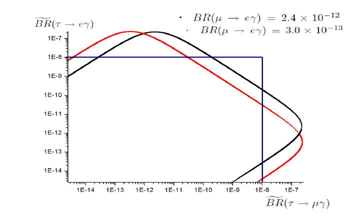
Figure 1: Branching ratios for $\tau\to\mu\gamma$ and $\tau\to e\gamma$ (normalised to leptonic decays as in eqn (15)) in the hypothetical cases that $\mu\to e\gamma$ was observed, with $BR(\mu\to e\gamma)=2.4\times 10^{-12}$ (upper rising-towards-the-left black line), or $BR(\mu\to e\gamma)=3.0\times 10^{-13}$ (lower rising-towards-the-left red line). The correlation arises from the assumptions discussed after eqn (37). The $\widetilde{BR}$s are estimated with eqn (59). The estimated sensitivity of superB factories is outside the (blue) rectangle. This plot can also be interpreted as an upper bound on the $\widetilde{BR}$s which are consistent with a $\mu\to e\gamma$ bound: the allowed region is to the left and below the diagonal line sloping-up-to-the-left. The horizontal and vertical cutoffs are uncertain because they are determined by our estimate of $C_{\nu}^{X}$.

To reconstruct the singlet masses with equation(21), requires the neutrino mass matrix ${\bf m_{\nu}}$ and the whole ${\bf P}$ matrix. However, in the approximation (17), neither the ${\bf Y}^{\nu}$ eigenvalues nor the third mixing angle of $V_{L}$ can be determined from rare decays (degenerate sneutrinos [28, 6] could give additional information). Our reconstructed singlet masses therefore depend on the unknown $\theta_{VL12},y_{1}$ and $y_{2}$. We can estimate ranges for these parameters which give $M_{1}\sim 10^{10}$ GeV, as would be suitable for thermal leptogenesis.

The inverse mass matrix of the singlets is given in equation(21), as a function of the “known” doublet parameters. When one eigenvalue of a $3\times 3$ matrix ${\bf M}$ vanishes, the two remaining eigenvalues are given by [29]

$$M_{1},M_{2}=\frac{1}{2}\left[\mbox{Tr}[{\bf M}]\pm\sqrt{(\mbox{Tr}[{\bf M}])^{2}-4({M}_{11}{M}_{22}+{M}_{11}{M}_{33}+M_{22}M_{33}-M_{23}^{2}-{M}_{12}^{2}-{M}_{13}^{2})}\right]$$ (38)

We find that for generic choices of the mixing angles in $V_{L}$, the singlet masses $M_{1}$ and $M_{2}$ have the form $\sim v^{2}y_{i}^{2}/\overline{m}$, as plotted in figure 2, where $\overline{m}=\sqrt{\Delta m^{2}_{sol}}+\sqrt{\Delta m^{2}_{atm}}$. This is unsurprising, since the light masses corresponding to eqn (6) are much more degenerate than the squared eigenvalues of ${\bf Y}^{\nu}$. So a given $M_{I}$ is usually controlled by a single $y_{i}^{2}$, and the singlet mixing angles in $V_{R}$ are generically small. That is, $V_{R}$ usually can be written as a rotation matrix with small mixing angles multiplied by either the identity matrix or a permutation. We find that we can always choose Yukawa eigenvalues to obtain $M_{1}\sim 10^{10}~{}{\rm GeV}$, as suggested for thermal leptogenesis. This tells us that even if all rare decays were measured, the lightest singlet mass is not determined, so whether it has a value suitable for leptogenesis is not known.

To reproduce, in this model, the two singlet case of section 3, can be achieved by setting $\theta_{WL12}$ and $\theta_{WL13}$ in $W_{L}$ to zero. Then $y_{1}$ becomes irrelevant for the reconstruction, $\theta_{WL23}$ plays the role of $\theta_{WL}$ in the two singlet model. In this limit, $M_{1}$ depends quadratic on $y_{2}$.

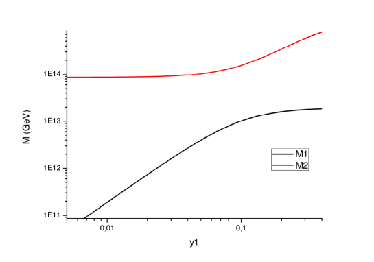
Figure 2: General dependence, in the three-singlet model where $1/M_{3}\to 0$, of the singlet masses on the smallest Yukawa eigenvalue $y_{1}$. In this plot, $y_{2}=.01$ and $y_{3}=1$. The angles in $W_{L}$ were taken similar to those of $U$: $\theta_{WL13}=.18$, $\theta_{WL12}=.6$, and $\theta_{WL23}=.6$. Different values of the mixing angles can shift the normalisation of the axes.

An interesting question is whether we can distinguish between the two or three singlet models by measuring rare decay rates? Not unambiguously. If the measured branching ratios disagree with the predictions of the two singlet see-saw model, it can be excluded. However, if the branching ratios agree with the two singlet predictions, we cannot exclude the three singlet model, which can fit every constellation of branching ratios that is possible in the two singlet model.

Consider now the case where the smallest neutrino mass is small, but non-zero. The Majorana mass eigenvalue $M_{3}$ is no longer infinite, but should remain larger than the other two mass eigenvalues $M_{1,2}$. However, it is not transparent to analytically determine the values of the smallest mass, as a function of other parameters, for which this condition is satisfied. A more stringent condition that ensures the validity of our reconstruction is that, in equation (21), for each component of $\bf M^{-1}$, the effect of $m_{1}$ is small compared to the effects of the other two mass eigenvalues (normal hierarchy):

$$[{\bf D_{\nu}}^{-1}{W_{L}}]_{I1}m_{1}[{W}_{L}^{T}{\bf D}_{\nu}^{-1}]_{1J}<<[{\bf D_{\nu}}^{-1}{W_{L}}]_{Ik}m_{k}[{W}_{L}^{T}{\bf D}_{\nu}^{-1}]_{kJ}\,\,\,\,\mbox{ where }k=2,3\mbox{ and }I,J=1,2,3$$ (39)

Those conditions imply that the reconstruction done in this section is valid if $m_{1}<<m_{k}$, except when $W_{L}$ is almost a diagonal or permutation matrix. In this special case, the contributions of $m_{2,3}$ are multiplied by a small mixing angle or by the cosine of a almost $\pi/2$ angle, whereas the contribution of $m_{1}$ is multiplied by almost one, so the reeconstruction is valid for

$$\frac{m_{1}}{m_{k}}<<\theta_{WLi}^{2}\mbox{ or }<<\left(\theta_{WLi}-\frac{\pi}{2}\right)^{2}$$ (40)

4.2 One zero Yukawa eigenvalue

In this section, we briefly discuss the case where the lightest neutrino mass vanishes, $m_{\nu min}\rightarrow 0$, because one Yukawa eigenvalue, which we take to be $y_{1}$, goes to zero.

Equation (20) can be rewritten:

$$W_{L}{\bf D}_{m}W_{L}^{T}={\bf D}_{\nu}V_{R}{\bf D_{M}}^{-1}V_{R}^{T}{\bf D}_{\nu}v_{u}^{2}$$ (41)

where ${\bf D_{\nu}}$ has only two non zero entries on the diagonal and therefore the right hand side of this equation has only a $2\times 2$ sub matrix with non-zero entries. Furthermore, we know that the doublet neutrino mass eigenstates in ${\bf D}_{m}$ do not couple to the vanishing first Yukawa eigenvalue $y_{1}$. Therefore the two angles $\theta_{W12}$ and $\theta_{W13}$ are identically zero, and a $2\times 2$ singlet inverse mass matrix can be reconstructed using eqn (21). However, ${\bf D}_{M}^{-1}$ on the right hand side of eqn (41) still contains the three singlet masses. Three equations do not determine three mass eigenvalues and three mixing angles, so the whole high energy Lagrangian cannot be reconstructed.

This limit reduces to the case of two right handed neutrinos. The right hand side of equation (41) can be rewritten in terms of two ”effective” mass eigenvalues and one ”effective” mixing angle. Of course the effective values are functions of the three initial mass eigenvalues and the three mixing angles, but we can only determine the effective values. So we cannot observe any difference between the two models unless we can measure the operator ${\bf[d]}$. With this operator we can distinguish between the two models, but we cannot perform a complete reconstruction, as discussed in the following section.

5 More singlets and the inverse seesaw

In this section, we consider the prospects for testing, in principle, the seesaw model we reconstructed. We suppose an ideal world where the matrices ${\bf P},[{\bf m}]$ and $[{\bf d}]$ could be exactly determined. Then from ${\bf P}$ and $[{\bf m}]$, one can compute ${\bf d}$, and compare its elements to their measured values.

As a first example, consider a model with three singlets, and $m_{1}=y_{1}=0$. To be concrete, we take a normal hierarchy for the light neutrino masses; a similar reasoning applies for the inverse hierarchy, but in a different two-dimensional subspace of doublet flavour space.

In the singlet basis where ${\bf Y^{\nu}}^{\dagger}{\bf Y^{\nu}}$ is diagonal (with eigenvalues $\{0,y_{2},y_{3}\}$), we can reconstruct a $2\times 2$ submatrix, which we call ${\bf{\widetilde{M}}}^{-1}$, of the “true” $3\times 3$ matrix

$${\bf M}^{-1}=\left[\begin{array}[]{ccc}M^{-1}_{11}&M^{-1}_{12}&M^{-1}_{13}\\ M^{-1}_{21}&\widetilde{M}^{-1}_{22}&\widetilde{M}^{-1}_{33}\\ M^{-1}_{31}&\widetilde{M}^{-1}_{32}&\widetilde{M}^{-1}_{33}\\ \end{array}\right]~{}~{}~{},$$ (42)

We imagine this matrix is reconstructed from ${\bf P}$ and $[{\bf m}]$, as was discussed in section 4: one obtains the Yukawa eigenvalues (two non-zero) and the $3\times 3$ rotation matrix $V_{L}$ from ${\bf P}$. This gives the $2\times 2$ matrix $W_{L}$, which can be substituted into eqn (21) whose left-hand-side is $\widetilde{{\bf M}}^{-1}$.

The matrix ${\bf{\widetilde{M}}}^{-1}{\bf{\widetilde{M}}}^{*-1}$, together with $W_{L}$ and ${\bf D}_{\nu}$, can combined to give a “prediction” for $[{\bf d}]$, expressed in the neutrino mass basis:

$$[{\bf d}]{\Big{|}}_{pred}=W_{L}^{\dagger}{\bf D}_{\nu}{\bf{\widetilde{M}}}^{-1}{\bf{\widetilde{M}}}^{*-1}{\bf D}_{\nu}W_{L}$$ (43)

which differs from the “true” expression for $[{\bf d}]=W_{L}^{\dagger}{\bf D}_{\nu}{\bf M}^{-1}{\bf M}^{*-1}{\bf D}_{\nu}W_{L}$,

$$[{\bf d}]{\Big{|}}_{true}=W_{L}^{\dagger}{\bf D}_{\nu}\left({\bf{\widetilde{M}}}^{-1}{\bf{\widetilde{M}}}^{*-1}+\left[\begin{array}[]{cc}|M^{-1}_{12}|^{2}&M^{-1}_{12}M^{*-1}_{13}\\ M^{*-1}_{12}M^{-1}_{13}&|M^{-1}_{13}|^{2}\end{array}\right]\right){\bf D}_{\nu}W_{L}$$ (44)

which would correspond to the measured value, in our ideal world. It is clear that the reconstructed and true matrices differ, and the determinant of the difference is zero. We could repeat this exercise with four singlets, and find that the determinant of the difference matrix is non-zero. So in principle, in this best of ideal worlds, it is possible to find traces of additional singlets, even when their (Yukawa) interactions with the Standard Model are irrelevant to LFV and neutrino masses.

Notice that since $y_{1}=0$, we not can get access to $[{\bf M}^{-1}]_{11}$, and therefore can not determine the mass of the singlet $N_{1}^{c}$. So a complete reconstruction is not possible. This is as expected, because in the limit where $[{\bf M}^{-1}]_{1i}\to 0$,for $i\neq 1$, the singlet $N_{1}^{c}$ is decoupled from the Standard Model.

Finally, consider an “inverse seesaw” model, with two singlets $N_{I}$ of lepton number -1, and two singlets $S_{I}$ of lepton number 1, who have no Yukawa couplings but a small majorana mass matrix $\mu$_IJ:

$${\cal L}_{inverse}=y^{e}_{{\alpha}}\overline{\ell}^{\alpha}H^{*}_{d}e_{R}^{\alpha}+\overline{\ell}^{\alpha}H^{*}_{u}[{\bf Y^{\nu}}^{*}]_{\alpha I}N_{I}+{M}_{I}\overline{S}_{I}N_{I}+\frac{\mu_{IJ}}{2}\overline{S^{c}}_{I}S_{J}+h.c.$$ (45)

This is a special case of a four-singlet model with only two non-zero eigenvalues in ${\bf Y^{\nu}}$, and we just argued that a generic such four-singlet model could not be reconstructed even in the best of all worlds. Nonetheless, the supersymmetric inverse seesaw is reconstructable. From ${\bf P}$ and $[{\bf d}]$, which are defined as in the ordinary seesaw in eqns (18) and (11), one can obtain ${\bf Y^{\nu}}$ and ${\bf M}$. Then from the effective light neutrino mass matrix

$$[{\bf m}]={\bf{\bf Y^{\nu}}}{\bf M}^{-1}\mu\,{\bf M}^{-1}{\bf Y^{\nu}}^{T}v_{u}^{2}~{}~{}~{},~{}~{}~{}~{}$$ (46)

one can obtain $[\mu]$. This could suggest that the supersymmetric inverse seesaw could fit any observations of neutrino mass, mixing and non-unitarity, as well as $\ell_{\alpha}\to\ell_{\beta}\gamma$ [8, 30]. An independent determination of the singlet masses(at a collider), could test this model.

6 Summary and Discussion

We considered simple toy supersymmetric seesaws (the lightest neutrino was taken massless) with 2,3 and 4 heavy singlets, and usually real parameters. We were interested in the properties of a model that allow it to be reconstructed in principle, so we studied the prospects of reconstructing the high-scale parameters of these models from observations at or below a TeV. We imagine that such observations could give us access to three matrices in doublet lepton flavour space (see eqns (18), (5), and (11)) :

$${\bf P}=V_{L}^{\dagger}D^{2}_{\nu}V_{L}~{}~{}~{},~{}~{}~{}[{\bf m}]={\bf{\bf Y^{\nu}}}{\bf M}^{-1}{\bf Y^{\nu}}^{T}v_{u}^{2}~{}~{}~{},~{}~{}~{}~{}[{\bf d}]={\bf Y^{\nu}}{\bf M}^{-1}{\bf M}^{-1*}{\bf Y^{\nu}}^{\dagger}$$

It is a straightforward exercise in linear algebra to show that, if ${\bf Y^{\nu}}$ is an invertible $3\times 3$ matrix, then from any pair of the above three matrices, a $3\times 3$ matrix ${\bf M}$ can be obtained. This gives the masses and mixing angles of three singlets $\{N_{I}\}$. Therefore, measuring the third of the above three matrices could test the model.

This programme to test the seesaw suffers from a serious practical problem, which is that ${\bf P},{\bf m}$ and ${\bf d}$ cannot be measured exactly, if at all. We attempted to circumvent this problem by neglecting phases, and by using “reasonable” theoretical expectations (such as that the ${\bf Y^{\nu}}$ eigenvalues are hierarchical) for unknown parameters. We also take the lightest neutrino mass to be zero.

Then we studied the question of “principle”, whether it is possible to determine the number of singlets participating in the seesaw, and reconstruct their properties.

• Since the lightest neutrino was taken massless, only two singlets are requireed to reproduce the light neutrino mass matrix. As shown by Ibarra [5], the seesaw model with two singlets, and two eigenvalues for ${\bf Y^{\nu}}$, is testable. In particular, as discussed in section 3 it predicts a discrete set of possible rates for $\tau\to\ell\gamma$, given the rate for $\mu\to e\gamma$. If the $BR(\mu\to e\gamma)$ is taken at the current bound of $2.4\times 10^{-12}$, then for a normal hierarchy of light neutrino masses, one of the $BR(\tau\to\ell\gamma)\mathrel{\vbox{\hbox{$>$}\nointerlineskip\hbox{$\sim$}}}10^{-8}$ should be visible at a super-B factory (for susy parameters as described in the Appendix, giving rate expectations as in eqn (59)). In the case of an inverse hierarchy, a similar situation could arise, or — unfortunately— both $\tau\to\ell\gamma$ decays could be out of the reach of super-B factories.

  To reconstruct the singlet sector of this model, we assume the largest ${\bf Y}_{\nu}$ eigenvalue to be 1, and fix the smaller by setting the lighter singlet mass $\sim 10^{10}$ GeV, for thermal leptogenesis.

• The three singlet model can have a massless light neutrino in two limits: either one of the singlets is very heavy ($M_{3}^{-1}\to 0$), or there are only two non-zero eigenvalues to in ${\bf Y^{\nu}}$ (so $y^{\nu}_{1}\to 0$).

  • The first case, where the $3\times 3$ ${\bf Y^{\nu}}$ is invertible, is in principle a reconstructable model, allowing to obtain the mixing angles and masses of the three singlets. As discussed in section 4 it differs from the two-singlet model, in that the three angles of $V_{L}$ are independent. This means that knowing the rate for one Lepton Flavour Violating decay, such as $\mu\to e\gamma$, does not determine the other two. Instead, for hierarchical ${\bf Y^{\nu}}$ eigenvalues, knowing two lepton-flavour-violating branching ratios, allows to predict the third.

    However, as discussed in section 4, this case is not a very realistic limit: if $M_{3}$ is sufficiently large that it contributes negligeably to the light neutrino masses, it is unlikely to be present in loop corrections to the sneutrino masses. This means that the Yukawa couplings of $N_{3}$ would not contribute to ${\bf P}$, which would therefore effectively have only two non-zero eigenvalues (see eqn (36)).

  • The second case, where the smallest of the three Yukawa eigenvalues is negligeable, is equivalent to the two-singlet case, except that the $2\times 2$ singlet inverse mass matrix that one reconstructs using a $2\times 2$ ${\bf Y^{\nu}}$ matrix in eqn (21), is only a $2\times 2$ submatrix of the full inverse mass matrix ${\bf M}^{-1}$. As discussed in section 5, models which all have two non-zero ${\bf Y^{\nu}}$ eigenvalues, but have two, three or four singlets, are in principle distinguishable because they give different predictions for ${\bf d}$. However, it is not possible to fully reconstruct the singlet sector. This is straightforard to see in the limit where the additional singlets are decoupled, because they interact only via the vanishing Yukawa eigenvalue.

• Four singlet models are in general not reconstructible — that is, the singlet masses cannot be obtained. However, if the singlet mass matrix is of the “inverse seesaw” type, it is reconstructible, in principle, from the sneutrino mass matrix (${\bf P}$) the light neutrino mass matrix, and the operator ${\bf d}$ given in eqn (11).

Almost any observed rates for $\ell_{\alpha}\to\ell_{\beta}\gamma$ can be compatible with the three-or-more singlet supersymmetric seesaw [3, 31]. The precise relation between the $\ell_{\alpha}\to\ell_{\beta}\gamma$ rates, and the seesaw parameters depends on various aspects and scales of the soft-supersymmetry-breaking mechanism. To circumvent the (not very well delimited) uncertainties resulting from these “soft” assumptions, we estimated the $\ell_{\alpha}\to\ell_{\beta}\gamma$ rates using a basic Minimal-Flavour-Violation-like parametrisation (eqn (13)), which could give a “lowest order” decription of the supersymmetric seesaw — and of several other models.

The coefficient ${\bf X}_{L}$ of the electromagnetic dipole operator (see eqn (12)) is a matrix with indices in doublet and singlet charged lepton flavour spaces. We assumed that its flavour-changing elements were proportional to ${\bf Y}^{e\dagger}\hat{{\bf P}}$, where ${\hat{\bf P}}$ is a new “spurion”, or matrix in doublet lepton flavour space. A first approximation to the supersymmetric seesaw is to take $\hat{{\bf P}}={\bf Y}^{\nu}{\bf Y}^{\nu\dagger}$. We further assumed that the eigenvalues of $\hat{{\bf P}}$ were hierarchical, such that the largest contributions to flavour changing matrix elements were always mediated by the largest eigenvalue. Finally, we assumed that the upper bound on $\mu\to e\gamma$ imposes an approximate zero in $\hat{{\bf P}}$. These assumptions, which could roughly describe the three-singlet supersymmetric seesaw, predict a relation between the $\tau\to\mu\gamma$ and $\tau\to e\gamma$ rates (see eqn (37) and figure 1).

The context of this study, was to explore the prospects of “reconstructing” the neutrino mass generation mechanism from coefficients of the effective Lagrangian. We focussed on supersymmetric seesaw models, because seesaws have many features which facilitate reconstruction. They contain New Physics at tree level, with well-separated mass scales. This means that the heavy propagators can be approximated as $1/m^{2}$ — which would be less straightforward, for instance, if the New Physics appeared in loops. In addition, all the new interactions and masses of the seesaw are flavoured and bilinear. This means that coefficients in the effective Lagrangian are constructed by matrix multiplication, so by combining “suitable” coefficients, one can solve for all the new matrices. This would be less simple, for instance, with R-parity violating trilinear couplings. Nonetheless, these nice features of the seesaw are not sufficient to ensure reconstructability, because we obviously cannot reconstruct New Physics in the limit where it decouples from us. It would be interesting to know what features are neccessary for a reconstructable model.

Acknowledgements

We thank Sebastien Descotes-Genon, Benjamin Guiot, and Christopher Smith for useful conversations.

Appendix

Our model is supersymmetric, so soft supersymmetry-breaking terms for the “sparticles” must be added to the Lagrangian obtained from the superpotential of eqn (1). These renormalisable terms are interesting for seesaw reconstruction, because loop processes can imprint traces of the high-scale theory upon them. A “Minimal Flavour Violation[20]-like” expectation for the mass-squared matrix of the slepton doublets $\{\widetilde{L}_{\alpha}\}$ could be of the form

$$[\widetilde{{\bf m}}^{2}]=C^{m}_{I}{\bf I}+C^{m}_{e}{\bf Y^{e}}{\bf Y^{e}}^{\dagger}+C^{m}_{\nu}{\bf Y^{\nu}}{\bf Y^{\nu}}^{\dagger}$$ (47)

because, in the high-scale theory described by the superpotential of eqn (1), the two spurions linking the $3$ and $\bar{3}$ of the doublet lepton space are ${\bf Y^{e}}{\bf Y^{e}}^{\dagger}$ and ${\bf Y^{\nu}}{\bf Y^{\nu}}^{\dagger}$. In the charged lepton mass eigenstate basis, ${\bf Y^{\nu}}{\bf Y^{\nu}}^{\dagger}$ generally gives off-diagonal elements of $[\widetilde{{\bf m}}^{2}]$, which would induce Lepton Flavour Violating (LFV) processes [32], such as $\ell_{\alpha}\to\ell_{\beta}\gamma$.

In a model for supersymmetry-breaking and flavour, the soft supersymmetry breaking parameters can be calculated, which gives a prediction for the coefficients $C^{m}_{x}$, and for corrections[33] to eqn (47). An estimate for $C^{m}_{\nu}$ can be obtained in gravity-mediated supersymmetry-breaking scenarios, because the soft breaking parameters are present at scales $\gg M$, where loops involving Higgses(higgsinos) and singlet (s)neutrinos give small contributions to the doublet slepton masses. These are approximately proportional to ${\bf Y^{\nu}}{\bf Y^{\nu}}^{\dagger}$, and are resummed by the renormalisation group equations. Assuming that, at some high scale $M_{X}\gg M_{I}$, the model contains universal soft terms of the form

$$\mathcal{L}_{soft}=\tilde{m}_{0}^{2}\tilde{L}_{\alpha}^{\dagger}\tilde{L}_{\alpha}+a_{0}(y^{e}_{\alpha}{\widetilde{L}}^{\alpha}\cdot H_{d}\widetilde{E^{c}}_{\alpha}+{\bf Y^{\nu}}_{\alpha I}\widetilde{L}^{\alpha}\cdot H_{u}\widetilde{N^{c}}_{I})+h.c.~{}~{},$$ (48)

then, in the leading log approximation, the slepton doublet soft masses $\widetilde{m}^{2}_{\alpha\beta}$ receive contributions [34, 35] of order

$$\Delta\widetilde{m}^{2}_{L\alpha\beta} \simeq -\frac{3m_{0}^{2}+a_{0}^{2}}{16\pi^{2}}\left[{\bf Y^{\nu}}\log\left(\frac{MM^{\dagger}}{M_{X}^{2}}\right){\bf Y^{\nu}}^{\dagger}\right]_{\alpha\beta}$$ (49)

where $\alpha,\beta$ are indices in the charged lepton mass basis. If one assumes that all the singlets can be decoupled at the same scale $M_{av}$, and that $\tilde{m}_{0}=a_{0}$, then one can approximate

$$\left[{\bf Y^{\nu}}\log\left(\frac{MM^{\dagger}}{M_{X}^{2}}\right){\bf Y^{\nu}}^{\dagger}\right]_{\alpha\beta}\to\left[{\bf Y^{\nu}}{\bf Y^{\nu}}^{\dagger}\right]_{\alpha\beta}\log\left(\frac{M_{av}^{2}}{M_{X}^{2}}\right)$$ (50)

which gives

$$C^{m}_{\nu}\simeq-\frac{m_{0}^{2}}{4\pi^{2}}$$ (51)

where we approximate the $\log\to 1$.

Lepton flavour violating radiative decays, $\ell_{\alpha}\to\ell_{\beta}\gamma$, proceed via the operator of eqn (12)

$$eX_{L\alpha\beta}\overline{e_{\alpha}}\sigma^{\mu\nu}P_{L}e_{\beta}F_{\mu\nu}+eX_{R\alpha\beta}\overline{e_{\alpha}}\sigma^{\mu\nu}P_{R}e_{\beta}F_{\mu\nu}~{}~{}~{},$$ (52)

at a rate given by eqn (15)

$$\widetilde{BR}(l_{\alpha}\to l_{\beta}~{}\gamma)=\frac{\Gamma(l_{\alpha}\to l_{\beta}~{}\gamma)}{\Gamma(\ell_{\alpha}\rightarrow\ell_{\beta}\nu_{\alpha}\bar{\nu}_{\beta})} = \alpha m_{\alpha}^{3}(|X_{L\alpha\beta}|^{2}+|X_{R\alpha\beta}|^{2})\frac{192\pi^{3}}{G_{F}^{2}m_{\alpha}^{5}}~{}~{}.$$ (53)

For a given weak-scale SUSY spectrum, the coefficients $X_{P\alpha\beta}$ can be calculated [36, 37] as a function of masses and mixing angles.

For $\alpha=\beta=\mu$, the dipole operator (12) also contributes to the anomalous magnetic moment of the muon

$$\frac{g-2}{2}\equiv a_{\mu}=4{\rm Re}\{X_{L\mu\mu}\}m_{\mu}$$ (54)

whose experimental determination [38] differs from the SM prediction by several standard deviations [39]. If this anomaly $\delta a_{\mu}\simeq 29\times 10^{-10}$ [39] is dominantly induced by the same New Physics diagram as $\ell_{\alpha}\to\ell_{\beta}\gamma$ (for instance, a chargino-slepton loop —see [40] for intuitive estimates of the various diagrams in the mass insertion approximation), then [41, 40]

$$\delta a_{\mu}\simeq\frac{g_{2}^{2}m_{\mu}^{2}}{32\pi^{2}\tilde{m}^{2}_{SUSY}}\tan\beta$$ (55)

and it is possible to “normalise” [42] the amplitude for $\ell_{\alpha}\to\ell_{\beta}\gamma$ by $\delta a_{\mu}$:

$$X_{L\alpha\beta} \sim X_{L\alpha\alpha}\frac{\widetilde{m}^{2}_{\alpha\beta}}{\widetilde{m}^{2}}\sim\frac{\delta a_{\mu}}{4m_{\mu}^{2}}m_{\alpha}\frac{\widetilde{m}^{2}_{\alpha\beta}}{\widetilde{m}^{2}}~{}~{}~{}.$$ (56)

For $\widetilde{m}^{2}=m_{0}^{2}$, $\widetilde{m}^{2}_{\alpha\beta}$ from eqn (49), and $X_{L\alpha\beta}$ of the form (13):

$${\bf X}_{L\alpha\beta}=m_{\alpha}C^{X}_{\nu}{\bf Y^{\nu}}{\bf Y^{\nu}}^{\dagger}~{}~{}~{},\alpha\neq\beta$$ (57)

this gives

$$C^{X}_{\nu} \sim \frac{\delta a_{\mu}}{16\pi^{2}m^{2}_{\mu}}~{}~{}~{},$$ (58)

and

$$\widetilde{BR}(l_{\alpha}\to l_{\beta}~{}\gamma) = \frac{3\alpha|\delta a_{\mu}|^{2}}{4\pi m_{\mu}^{4}G_{F}^{2}}{\Big{|}}[{\bf Y^{\nu}}{\bf Y^{\nu}}^{\dagger}]_{\alpha\beta}{\Big{|}}^{2}\simeq 10^{-6}{\Big{|}}[{\bf Y^{\nu}}{\bf Y^{\nu}}^{\dagger}]_{\alpha\beta}{\Big{|}}^{2}~{}~{}.$$ (59)

As is well-known [31, 43], the upper bound $\widetilde{BR}(\mu\to e\gamma)\leq 2.4\times 10^{-12}$ [22] restricts $[{\bf Y^{\nu}}{\bf Y^{\nu}}^{\dagger}]_{\mu e}\mathrel{\vbox{\hbox{$<$}\nointerlineskip\hbox{$\sim$}}}2\times 10^{-3}$, which implies, with the hierarchical assumption for ${\bf Y}^{\nu}$ of eqn (17), that there is a small entry in the mixing matrix $V_{L}$:

$$y_{3}^{2}|V_{L3\mu}V_{L3e}^{*}| \mathrel{\vbox{\hbox{$<$}\nointerlineskip\hbox{$\sim$}}} 2\times 10^{-3}~{}~{}~{}.$$ (60)

From current bounds [23] on $\tau\to\mu\gamma$ and $\tau\to e\gamma$, similar approximations give $|[{\bf Y^{\nu}}{\bf Y^{\nu}}^{\dagger}]_{\tau\ell}|\mathrel{\vbox{\hbox{$<$}\nointerlineskip\hbox{$\sim$}}}0.5$.

Notice that for $\tan\beta=10$, saturating the $(g-2)_{\mu}$ anomaly via eqn (55) gives $\tilde{m}_{SUSY}\sim 225$ GeV, a scale where colliders do not seem to find a supersymmetric menagerie. The estimate (59) scales with various parameters as

$$\widetilde{BR}(l_{\alpha}\to l_{\beta}~{}\gamma) \simeq \simeq 10^{-6}\left\{\,\left(\frac{\tan\beta}{10}\right)^{2}\left(\frac{225{\rm GeV}}{\tilde{m}_{SUSY}}\right)^{4}\right\}{\Big{|}}[{\bf Y^{\nu}}{\bf Y^{\nu}}^{\dagger}]_{\alpha\beta}{\Big{|}}^{2}~{}~{},$$ (61)

so changing a parameter by a factor of 2, can change the rare decay rates by an order of magnitude. The “approximate zero” of eqn (14), and the expectations which follow from it, relies on the factor in curly brackets in (61) being larger than $10^{-3}$.

References

- [1] P. Minkowski, Phys. Lett. B 67, 421 (1977); M. Gell-Mann, P. Ramond and R. Slansky, Proceedings of the Supergravity Stony Brook Workshop, New York, 1979, eds. P. Van Nieuwenhuizen and D. Freedman (North-Holland, Amsterdam); T. Yanagida, Proceedings of the Workshop on Unified Theories and Baryon Number in the Universe, Tsukuba, Japan 1979 (eds. A. Sawada and A. Sugamoto, KEK Report No. 79-18, Tsukuba); R. Mohapatra and G. Senjanovic, Phys. Rev. Lett. 44, 912 (1980).
- [2] T. Asaka, S. Blanchet, M. Shaposhnikov, “The nuMSM, dark matter and neutrino masses,” Phys. Lett. B631 (2005) 151-156. [hep-ph/0503065]. A. de Gouvea, J. Jenkins, N. Vasudevan, “Neutrino Phenomenology of Very Low-Energy Seesaws,” Phys. Rev. D75 (2007) 013003. [arXiv:hep-ph/0608147 [hep-ph]]. A. Donini, P. Hernandez, J. Lopez-Pavon, M. Maltoni, “Minimal models with light sterile neutrinos,” JHEP 1107 (2011) 105. [arXiv:1106.0064 [hep-ph]].
- [3] S. Davidson, A. Ibarra, “Determining seesaw parameters from weak scale measurements?,” JHEP 0109 (2001) 013. [hep-ph/0104076].
- [4] S. Davidson, “From weak scale observables to leptogenesis,” JHEP 0303 (2003) 037. [hep-ph/0302075].
- [5] A. Ibarra, “Reconstructing the two right-handed neutrino model,” JHEP 0601 (2006) 064. [hep-ph/0511136]. A. Ibarra, G. G. Ross, “Neutrino phenomenology: The Case of two right-handed neutrinos,” Phys. Lett. B591 (2004) 285-296. [hep-ph/0312138].
- [6] C. Cheung, L. J. Hall, D. Pinner, “Seesaw Spectroscopy at Colliders,” [arXiv:1103.3520 [hep-ph]].
- [7] J. A. Casas, A. Ibarra, F. Jimenez-Alburquerque, “Hints on the high-energy seesaw mechanism from the low-energy neutrino spectrum,” JHEP 0704 (2007) 064. [hep-ph/0612289].
- [8] A. Ibarra, E. Molinaro, S. T. Petcov, “Low Energy Signatures of the TeV Scale See-Saw Mechanism,” [arXiv:1103.6217 [hep-ph]].
- [9] S. Davidson, J. Garayoa, F. Palorini, N. Rius, “CP Violation in the SUSY Seesaw: Leptogenesis and Low Energy,” JHEP 0809 (2008) 053. [arXiv:0806.2832 [hep-ph]].
- [10] D. Wyler, L. Wolfenstein, “Massless Neutrinos in Left-Right Symmetric Models,” Nucl. Phys. B218 (1983) 205. R. N. Mohapatra, “Mechanism for understanding small neutrino mass in superstring theories”, Phys. Rev. Lett. 56 (1986) 561. M. C. Gonzalez-Garcia, J. W. F. Valle, “Fast Decaying Neutrinos And Observable Flavor Violation In A New Class Of Majoron Models,” Phys. Lett. B216 (1989) 360.
- [11] C. S. Aulakh, A. Melfo, A. Rasin, G. Senjanovic, “Seesaw and supersymmetry or exact R-parity,” Phys. Lett. B459, 557-562 (1999). [hep-ph/9902409].
- [12] R. Hempfling, “Neutrino masses and mixing angles in SUSY GUT theories with explicit R-parity breaking,” Nucl. Phys. B478 (1996) 3-30. [hep-ph/9511288]. E. J. Chun, S. K. Kang, “One loop corrected neutrino masses and mixing in supersymmetric standard model without R-parity,” Phys. Rev. D61 (2000) 075012. [hep-ph/9909429]. M. Hirsch, M. A. Diaz, W. Porod, J. C. Romao, J. W. F. Valle, “Neutrino masses and mixings from supersymmetry with bilinear R parity violation: A Theory for solar and atmospheric neutrino oscillations,” Phys. Rev. D62 (2000) 113008. [hep-ph/0004115]. S. Davidson, M. Losada, “Neutrino masses in the R(p) violating MSSM,” JHEP 0005 (2000) 021. [hep-ph/0005080], “Basis independent neutrino masses in the R(p) violating MSSM,” Phys. Rev. D65 (2002) 075025. [hep-ph/0010325].
- [13] G. C. Branco, L. Lavoura, M. N. Rebelo, “Majorana Neutrinos And Cp Violation In The Leptonic Sector,” Phys. Lett. B180 (1986) 264. A. Santamaria, “Masses, mixings, Yukawa couplings and their symmetries,” Phys. Lett. B305 (1993) 90-97. [hep-ph/9302301].
- [14] M. Raidal, A. van der Schaaf, I. Bigi, M. L. Mangano, Y. K. Semertzidis, S. Abel, S. Albino, S. Antusch et al., “Flavour physics of leptons and dipole moments,” Eur. Phys. J. C57 (2008) 13-182. [arXiv:0801.1826 [hep-ph]].
- [15] K. Nakamura et al. (Particle Data Group), J. Phys.G 37, 075021 (2010)
- [16] [ T2K Collaboration ], “Indication of Electron Neutrino Appearance from an Accelerator-produced Off-axis Muon Neutrino Beam,” [arXiv:1106.2822 [Unknown]].
- [17] A. De Gouvea, G. F. Giudice, A. Strumia, K. Tobe, “Phenomenological implications of neutrinos in extra dimensions,” Nucl. Phys. B623 (2002) 395-420. [hep-ph/0107156].
- [18] A. Broncano, M. B. Gavela, E. E. Jenkins, “The Effective Lagrangian for the seesaw model of neutrino mass and leptogenesis,” Phys. Lett. B552 (2003) 177-184. [hep-ph/0210271].
- [19] S. Antusch, C. Biggio, E. Fernandez-Martinez, M. B. Gavela, J. Lopez-Pavon, “Unitarity of the Leptonic Mixing Matrix,” JHEP 0610 (2006) 084. [hep-ph/0607020].
- [20] G. D’Ambrosio, G. F. Giudice, G. Isidori, A. Strumia, Nucl. Phys. B645 (2002) 155-187. [hep-ph/0207036].
- [21] M. L. Brooks et al. [MEGA Collaboration], “New limit for the family number nonconserving decay ,” Phys. Rev. Lett. 83 (1999) 1521 [arXiv:hep-ex/9905013].
- [22] J. Adam et al. [MEG collaboration], “New limit on the lepton-flavour violating decay ,” arXiv:1107.5547 [hep-ex].
- [23] B. Aubert et al. [BABAR Collaboration], “Searches for Lepton Flavor Violation in the Decays and ” Phys. Rev. Lett. 104 (2010) 021802 [arXiv:0908.2381 [hep-ex]]. K. Hayasaka et al. [Belle Collaboration], “New search for tau —¿ mu gamma and tau —¿ e gamma decays at Belle,” Phys. Lett. B 666 (2008) 16 [arXiv:0705.0650 [hep-ex]].
- [24] “The SuperB Physics Programme”, parrallel flavour talk thursday morning at the EPS Conference on HEP 2011 at Grenoble, http://eps-hep2011.eu/
- [25] M. Raidal, A. Strumia, “Predictions of the most minimal seesaw model,” Phys. Lett. B553 (2003) 72-78. [hep-ph/0210021]. W. -l. Guo, Z. -z. Xing, S. Zhou, “Neutrino Masses, Lepton Flavor Mixing and Leptogenesis in the Minimal Seesaw Model,” Int. J. Mod. Phys. E16 (2007) 1-50. [hep-ph/0612033].
- [26] S. Davidson, E. Nardi, Y. Nir, “Leptogenesis,” Phys. Rept. 466 (2008) 105-177. [arXiv:0802.2962 [hep-ph]].
- [27] L. Covi, M. Olechowski, S. Pokorski, K. Turzynski, J. D. Wells, “Supersymmetric mass spectra for gravitino dark matter with a high reheating temperature,” JHEP 1101 (2011) 033. [arXiv:1009.3801 [hep-ph]]. H. Baer, S. Kraml, A. Lessa, S. Sekmen, “Reconciling thermal leptogenesis with the gravitino problem in SUSY models with mixed axion/axino dark matter,” JCAP 1011 (2010) 040. [arXiv:1009.2959 [hep-ph]]. M. Fujii, T. Yanagida, “Natural gravitino dark matter and thermal leptogenesis in gauge mediated supersymmetry breaking models,” Phys. Lett. B549 (2002) 273-283. [hep-ph/0208191].
- [28] Y. Grossman, H. E. Haber, “Sneutrino mixing phenomena,” Phys. Rev. Lett. 78 (1997) 3438-3441. [hep-ph/9702421].
- [29] S. Davidson, M. Losada, N. Rius, “Neutral Higgs sector of the MSSM without R(p),” Nucl. Phys. B587 (2000) 118-146. [hep-ph/9911317].
- [30] W. Abdallah, A. Awad, S. Khalil, H. Okada, “Muon Anomalous Magnetic Moment and mu e gamma in B-L Model with Inverse Seesaw,” [arXiv:1105.1047 [hep-ph]]. D. V. Forero, S. Morisi, M. Tortola and J. W. F. Valle, “Lepton flavor violation and non-unitary lepton mixing in low-scale type-I seesaw,” arXiv:1107.6009 [hep-ph]. M. Malinsky, T. Ohlsson, Z. -z. Xing, H. Zhang, “Non-unitary neutrino mixing and CP violation in the minimal inverse seesaw model,” Phys. Lett. B679 (2009) 242-248. [arXiv:0905.2889 [hep-ph]].
- [31] C. Simonetto, A. Ibarra, “Minimal rates for lepton flavour violation from supersymmetric leptogenesis,” J. Phys. Conf. Ser. 259 (2010) 012077.
-
[32]
F. Borzumati, A. Masiero,
“Large Muon and electron Number Violations in Supergravity Theories,”
Phys. Rev. Lett. 57 (1986) 961.
For a review, see e.g. Y. Kuno, Y. Okada, “Muon decay and physics beyond the standard model,” Rev. Mod. Phys. 73 (2001) 151-202. [hep-ph/9909265]. - [33] see e.g., Z. Lalak, S. Pokorski, G. G. Ross, “Beyond MFV in family symmetry theories of fermion masses,” JHEP 1008 (2010) 129. [arXiv:1006.2375 [hep-ph]], and references therein.
- [34] I. Masina, “Lepton electric dipole moments from heavy states Yukawa couplings,” Nucl. Phys. B671 (2003) 432-458. [hep-ph/0304299].
- [35] Y. Farzan, M. E. Peskin, “The Contribution from neutrino Yukawa couplings to lepton electric dipole moments,” Phys. Rev. D70 (2004) 095001. [hep-ph/0405214].
- [36] J. Hisano, T. Moroi, K. Tobe, M. Yamaguchi, T. Yanagida, “Lepton flavor violation in the supersymmetric standard model with seesaw induced neutrino masses,” Phys. Lett. B357 (1995) 579-587. [hep-ph/9501407].
- [37] J. Hisano, T. Moroi, K. Tobe, M. Yamaguchi, “Lepton flavor violation via right-handed neutrino Yukawa couplings in supersymmetric standard model,” Phys. Rev. D53 (1996) 2442-2459. [hep-ph/9510309].
- [38] G. W. Bennett et al. [ Muon G-2 Collaboration ], “Final Report of the Muon E821 Anomalous Magnetic Moment Measurement at BNL,” Phys. Rev. D73 (2006) 072003. [hep-ex/0602035].
- [39] M. Davier, A. Hoecker, B. Malaescu, Z. Zhang, “Reevaluation of the Hadronic Contributions to the Muon g-2 and to alpha(MZ),” Eur. Phys. J. C71 (2011) 1515. [arXiv:1010.4180 [hep-ph]].
- [40] M. Graesser, S. D. Thomas, “Supersymmetric relations among electromagnetic dipole operators,” Phys. Rev. D65 (2002) 075012. [hep-ph/0104254].
- [41] T. Moroi, “The Muon Anomalous Magnetic Dipole Moment in the Minimal Supersymmetric Standard Model,” Phys. Rev. D 53 (1996) 6565 [Erratum-ibid. D 56 (1997) 4424] [arXiv:hep-ph/9512396].
- [42] J. Hisano and K. Tobe, “Neutrino masses, muon g-2, and lepton-flavour violation in the supersymmetric see-saw model,” Phys. Lett. B 510 (2001) 197 [arXiv:hep-ph/0102315].
- [43] see e.g. the discussion in [14], and references therein.