Diffusion-limited reactions on disordered surfaces with continuous distributions of binding energies

Abstract

We study the steady state of a stochastic particle system on a two-dimensional lattice, with particle influx, diffusion and desorption, and the formation of a dimer when particles meet. Surface processes are thermally activated, with (quenched) binding energies drawn from a continuous distribution. We show that sites in this model provide either coverage or mobility, depending on their energy. We use this to analytically map the system to an effective binary model in a temperature-dependent way. The behavior of the effective model is well-understood and accurately describes key quantities of the system: Compared with discrete distributions, the temperature window of efficient reaction is broadened, and the efficiency decays more slowly at its ends. The mapping also explains in what parameter regimes the system exhibits realization dependence.

Keywords: stochastic particle dynamics (theory), disordered systems (theory), stochastic processes (theory), catalysis

1 Introduction

The interplay of diffusive transport and quenched random reaction rates poses some of the most intriguing problems in the statistical physics of disordered systems [1]. While the simple case of single-particle diffusion in random media is reasonably well understood [2, 3], already the linear dynamics that arises from adding an autocatalytic reaction term to the diffusion (heat) equation generates complex, intermittent spatio-temporal patterns [4] that have only recently become tractable by rigorous analysis [5].

In the present paper we consider a particular variant of this general class of problems, which is motivated by the physics of heterogeneous catalysis on disordered surfaces [6, 7, 8, 9]. We study a large (but finite) two-dimensional lattice system with stochastic particle dynamics, including influx, desorption, diffusion and pairwise reaction upon meeting. The rates of desorption and diffusion are subject to quenched disorder. An important realization of this type of dynamics are chemical reactions on dust grains in interstellar clouds, for a review see [10]. In the paradigmatic reaction in this context, hydrogen atoms from the gas phase collide with and stick to a dust grain, they diffuse on its surface, and if two of them meet, they form an $\mathrm{H}_{2}$ molecule [11, 12]. The key quantity of such systems is their steady-state efficiency, i.e., the fraction of incoming particles which leave due to the reaction (as opposed to thermal desorption of a particle before it takes part in a reaction)—the significance for applications is evident. All other parameters being fixed, this is typically a function of the system temperature, and high efficiency is limited to a specific temperature range. Below this range, particles become immobile and can no longer react, while above they are thermally emitted too quickly.

In previous work, we and others have first studied the system with homogeneous rates for all processes, when one can obtain analytical results [13, 14, 15, 16, 17]. However, spatial inhomogeneities in the process rates are of theoretical interest and of importance for applications. We have therefore started a systematic analysis of the effect of disorder in the local rates of hopping and desorption. In [18], we considered a binary model that consists of a lattice of adsorption sites, each associated with one of two possible binding energies, and labeled as standard (“shallow”) and strong-binding (“deep”) sites, respectively. All effects on the efficiency seen in kinetic Monte Carlo (KMC) simulations of this system have been well-understood, and we have provided thorough explanations in terms of microscopic processes, complemented by analytical mean-field results. This binary case is important both as a starting point for theory as well as for applications, where one can often naturally identify shallow and deep sites. Note that even in this case, there are no exact analytical results beyond a mean-field description (particularly not for finite system size).

The generalization to the more generic case of continuous distributions of binding energies now naturally suggests itself for applications, and it is of fundamental interest to the theory of disordered systems, where it is well known that the nature of the disorder distribution (i.e., discrete vs. continuous) may qualitatively affect the behavior. For example, for the random field Ising model [19, 20], a bimodal distribution of the local field strength has been suggested to give rise to a first-order phase transition, whereas other, continuous, distributions do not [21] (see also [22] and references therein for an account of the still ongoing debate). Similarly, in the context of random Schrödinger operators the shape of the Lifshitz tails in the electronic density of states is known to differ markedly between discrete and continuous (bounded) disorder distributions [23].

In this paper we extend the analysis of diffusion-limited surface reactions from the binary case [18] to continuous distributions. The central result of our work is the existence of a simple mapping from the case of binding energies drawn from a continuous distribution to an effective binary model as described above. This mapping is highly intuitive and we argue for its validity supported by strong numerical evidence. The binary model in turn is well-understood and, using mean-field methods, easily soluble (analytically in principle, and using minimal numerical techniques in practice) for the steady-state coverage and efficiency. Note that the mapping depends on the system temperature, which is responsible for the fact that the system’s behavior is qualitatively different from the genuinely discrete distribution case studied previously. Together we thus provide both a detailed understanding of the physics of stochastic particle systems with disordered binding energies as well as a straight-forward way to calculate key quantities of practical interest. Moreover, it is a question of general importance for the analysis of stochastic particle systems if (and how) a continuous distribution may be effectively replaced by a simpler discrete one. For the particular system studied here, we answer this question comprehensively (and affirmatively). The accessible microscopic explanations may also provide hints for the possibility of such a mapping for related models from other fields.

The paper is organized as follows. In section 2 we introduce the model and define the notation and terminology. We also describe the simulation techniques and the parameters used. We give a brief review of the necessary background for the corresponding homogeneous and binary systems in section 3. In section 4 we present the effective binary model and derive the mapping to it. We show the excellent agreement of the model results with those of KMC simulations. We also analyze the shape of the efficiency tails and the issue of sample-to-sample fluctuations. Lastly, we summarize our findings and their implications in the conclusions (section 5).

2 Model and simulation

2.1 Definition of the model

The model surface is a two-dimensional square lattice of $S$ sites with periodic boundary conditions. On this lattice we consider the dynamics of particles of a single species. They impinge onto the lattice at a homogeneous rate $f$ per site. If a site is already occupied, the impinging particle is rejected. In the context of surface chemistry this is known as Langmuir-Hinshelwood (LH) rejection [24].

Particles explore the lattice by hopping to neighboring sites with an (undirected) rate $a_{s}$, and they can spontaneously leave a site by desorption with rate $W_{s}$. Both rates depend on the current particle position $s$ (but not on its neighborhood). If two particles meet on one site, they react to form a dimer and leave the system immediately. We denote the total rate of these reaction events in the system by $R$. The key quantity of such a system is the efficiency $\eta$, defined as the ratio between the number of particles that react and the total number of impinging particles, when the system is in a steady state,

$$\eta=2R/(fS).$$ (1)

We denote the steady-state number of particles on the grain by $N$, such that the coverage reads $\theta=N/S$.

In view of possible applications (cf. section 1), we choose the rates $W_{s}$ and $a_{s}$ to be thermally activated by a system temperature $T$. The activation energy for desorption or binding energy at site $s$ is denoted $E_{W_{s}}$. Similarly, hopping from that site has an activation energy $E_{a_{s}}$. All rates share the attempt frequency $\nu$, so that

$$W_{s}=\nu\exp\left(-\frac{E_{W_{s}}}{T}\right),\qquad\text{and}\quad a_{s}=\nu\exp\left(-\frac{E_{a_{s}}}{T}\right).$$ (2)

Here and in the following energies are measured in temperature units.

In principle, $E_{a_{s}}$ could be independent of $E_{W_{s}}$, but we want to ensure detailed balance. The simplest way to achieve this is by choosing $W_{s}/a_{s}=\mathrm{const}$, and we will employ this choice throughout. Equivalently, $E_{W_{s}}-E_{a_{s}}=\Delta E$, where $\Delta E$ is a constant (independent of the site) describing the additional energy needed for desorption on top of the local transition state energy. The average number of sites visited by a single particle before desorption becomes then independent of the local rates and $\approx a_{s}/W_{s}$ (for $W_{s}\ll a_{s}$). Finally, the binding energy $E_{W_{s}}$ for each lattice site $s$ is drawn once from a probability density function (PDF) $\rho(E_{W})$ and remains fixed (quenched disorder realization). A one-dimensional cut through such an energy landscape is sketched in figure 1. Without desorption, this construction of the energy landscape and the associated hopping rates is known as the “random trap model” [2].

Figure 1: One-dimensional cut through the energy landscape of our model.

2.2 Kinetic Monte Carlo simulation

Our reference point for the system behavior is provided by extensive kinetic Monte Carlo simulations. The standard algorithm proceeds as follows (cf. [25] for a review). We keep track of the full microscopic dynamics of continuous-time random walkers [26] with standard exponential waiting time distributions. In each simulation step, the current system configuration determines the list of possible elementary processes (influx, as well as desorption and nearest-neighbor hopping of all particles on the lattice) and their rates. By comparing a random number with the normalized partial sums of these rates we find the process to execute next. The simulation time is then advanced according to the total sum of rates and the configuration is updated.

For a given set of parameters, each realization of the model is characterized by the set of binding energies for all sites, which are independently drawn from a distribution. As characteristic examples of different types of distributions we consider a) the uniform distribution over a certain interval, with bounded support, b) the (shifted) exponential distribution, which has a low-energy cutoff, but a high-energy tail, and c) the normal distribution, with tails to low as well as high energies. The latter case is often appropriate for the description of systems where binding energies are affected by many different random influences.

Unless indicated otherwise, we simulate $10$ realizations for each set of parameters; and for each set, these realizations are drawn anew. The different realizations are not used for averaging, but rather so we can examine sample-to-sample variations due to quenched disorder. For a given realization, we wait for the system to reach the steady state. We then record the efficiency and the spatial distribution of reaction events, as well as the local and global coverage, over $10^{8}$ impingements.

For easy comparison, the model parameters are mostly taken from the astrophysical application mentioned before, as in our earlier work [18]. This guarantees that we observe interesting kinetic regimes, and, as a side effect, it highlights the relevance of our findings for applications. We use a quadratic square lattice of $S=100\times 100$ sites. The particle influx per site is $f=7.3\times 10^{-9}\ \mathrm{s}^{-1}$ (as obtained from typical values for the density and the thermal velocity of hydrogen atoms in interstellar clouds and from the density of adsorption sites on an amorphous carbon sample [27]). For the attempt frequency we choose the standard value of $\nu=10^{12}\ \mathrm{s}^{-1}$ which is commonly used throughout surface science. The energy landscape of the surface is described by the mean binding energy $\langle E_{W}\rangle=658\ \mathrm{K}$, and the mean diffusion barrier $\langle E_{a}\rangle=511\ \mathrm{K}$ (as found for hydrogen atoms on amorphous carbon [28]), with the difference $\Delta E=147\ \mathrm{K}$ being constant for all sites. The standard deviation of both energy distributions is denoted $\sigma$; we often use the value normalized by the mean binding energy, $\tilde{\sigma}=\sigma/\langle E_{W}\rangle$, which we vary between $10\%$ and $50\%$.

KMC simulations of similar and of more complex models have been performed in the astrophysical context [29]. Additional features include, among others, stochastic heating of the system, and accounting for the surface morphology (implying strongly correlated binding energies of adjacent sites), see, e.g., [30]. In contrast, the present work is not so much concerned with the concrete temperature ranges of efficient reaction for a certain set of parameters, but we rather strive for a coherent explanation of the underlying physics of the generic system.

3 Review of homogeneous and binary systems

In the remainder of this article we will repeatedly use concepts and our understanding of the homogeneous and binary case. Therefore we start with a brief review of these systems. We will consider steady-state conditions exclusively.

3.1 Homogeneous system

The homogeneous system is characterized by a single binding energy $E_{W}$ and a single hopping activation energy $E_{a}$ for all sites. It can be solved analytically using rate equations (and including LH rejection) [28, 27], or with the master equation (not including LH rejection) accounting for fluctuations as well [13, 14]. Results for coverage and efficiency, obtained using the rate equation approach (which is accurate for sufficiently large systems), are shown in figure 2. The efficiency is limited to a narrow window of temperatures, while the coverage monotonically decreases with increasing temperature. Note that while the coverage is very small above $T=14\ \mathrm{K}$, the reaction remains efficient as long as the mean number of sites the particles visit is still larger than the mean number of empty sites surrounding each particle.

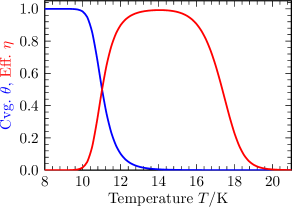
Figure 2: Coverage $\theta$ (blue) and efficiency $\eta$ (red) as functions of temperature $T$, in the homogeneous model described by a rate equation. Parameters are chosen as described in section 2.2, using the mean values of activation energies.

For later reference we recall the efficiency obtained in the rate equation approach [14],

$$\eta=1-\frac{(W+f)^{2}}{4fa}\left(\sqrt{1+\frac{8fa}{(W+f)^{2}}}-1\right).$$ (3)

This implies temperature bounds for the window of efficient reaction, where $\eta\geq 1/2$:

$$T^{\mathrm{low}}=\frac{E_{a}}{\ln(\nu/f)}$$ (4)

is the temperature below which particles arrive faster than they hop. Hence, the coverage is close to unity, leading to dominant LH rejection and low efficiency. Similarly,

$$T^{\mathrm{up}}=\frac{2E_{W}-E_{a}}{\ln(\nu/f)}$$ (5)

is the temperature above which desorption ends the typical particle residence before it can react. Therefore, in addition to the very low coverage, the efficiency is low as well. The temperature of maximal efficiency is approximately given by the average of these bounds and reads

$$T^{\mathrm{max}}=\frac{E_{W}}{\ln(\nu/f)}.$$ (6)

3.2 Binary system

The binary system is a particular case of the model described in section 2.1, where the distribution of binding energies is discrete and takes only two values $E_{W_{1}}$ or $E_{W_{2}}$, with $E_{W_{1}}<E_{W_{2}}$ [18]. The corresponding $S_{1}$ and $S_{2}$ sites are labeled “shallow” and “deep” for the lower and the higher binding energy, respectively, and subscripts only refer to the type of site $i$ here ($i=1,2$). In general, discreteness of particles and fluctuations in their number may render the mean-field description of the stochastic particle system at hand unsuitable, and thus rate equations overestimate the efficiency [31, 14, 32, 33, 15, 34]. For binary systems of sufficient size as treated here, these effects are negligible, and one finds excellent agreement between the efficiency seen in KMC simulations and obtained from a rate equation description [18]. The steady-state equations of this model for the number of particles $N_{i}$ on sites of type $i$ read

$$\frac{\mathrm{d}N_{1}}{\mathrm{d}t} =f(S_{1}-N_{1})-W_{1}N_{1}-A_{1}N_{1}(S_{2}-N_{2})-A_{1}N_{1}N_{2}$$ (7)

$$\quad-2A_{1}N_{1}^{2}+A_{2}N_{2}(S_{1}-N_{1})-A_{2}N_{1}N_{2}=0,$$

$$\frac{\mathrm{d}N_{2}}{\mathrm{d}t} =f(S_{2}-N_{2})-W_{2}N_{2}-A_{2}N_{2}(S_{1}-N_{1})-A_{2}N_{1}N_{2}$$

$$\quad-2A_{2}N_{2}^{2}+A_{1}N_{1}(S_{2}-N_{2})-A_{1}N_{1}N_{2}=0,$$

where the sweeping rate $A_{i}=a_{i}/S$ governs the rate of reaction due to hops from sites of type $i$ (not an elementary process). The simple expression for $A_{i}$ results from the fact that for disordered systems, a consistent rate equation description has to assume that particles can hop from any site to any other [18]. Note that this is not mandatory for homogeneous systems, where using $A=a/S$ to describe nearest-neighbor hopping presents an unsubstantiated approximation [15, 16, 17]. While (7) are exactly solvable by finding the real positive root of a third-order polynomial, the result is cumbersome, hence we prefer a direct numerical solution throughout.

The reaction terms provide the production rate of the process. Adding up all terms proportional to the $A_{i}$ in $\mathrm{d}N/\mathrm{d}t=\mathrm{d}N_{1}/\mathrm{d}t+\mathrm{d}N_{2}/\mathrm{d}t$, mere hopping terms (not leading to a reaction) cancel. Since the reaction consumes two particles, we obtain the rate at which particles are removed by the reaction as

$$2R=2A_{1}N_{1}^{2}+2A_{2}N_{2}^{2}+2(A_{1}+A_{2})N_{1}N_{2},$$ (8)

where the three contributions correspond to reactions triggered by hopping between shallow sites, between deep sites, and from one type of site to the other, respectively. Relating this to the total particle influx $f(S_{1}+S_{2})=fS$ yields the efficiency $\eta=2R/(fS)$.

In this system, whenever there is a substantial efficiency of reaction, the two types of sites play entirely different roles: Shallow sites provide mobility to the particles—by allowing them to move easily and quickly, they can sweep large parts of the system. Deep sites, however, provide coverage—while particles stuck there hardly ever move, they are also prevented from leaving the system. Acting together, the shallow sites allow particles to traverse over many sites of the system, funneling them to deep sites eventually, where they likely meet a stuck particle to react with and contribute to the efficiency. As a result, deep sites are, on average, covered half of the time, since occupying an empty site takes as long as emptying an occupied one by a reaction.

Compared with this process, reactions taking place on shallow sites are very unlikely. As soon as particles on such sites become mobile enough, they may sweep over shallow sites only, which are sparsely populated compared with deep sites. Hence they most likely end up in a deep well which is already occupied (leading to a reaction), or the well is newly occupied by the incoming particle, now stuck and waiting for the next one. Likewise, reaction by hops between deep sites is prevented since particles only become mobile at very high temperatures, when the overall coverage (governed by $f/W$) is low, and traversal over shallow wells is a leak through which particles leave immediately.

The different role that shallow and deep sites play in this model is highlighted by figure 3, obtained by solving (7). For a wide range of parameters, the separate efficiency windows corresponding to homogeneous systems of either type of site are “bridged” to one broad efficiency window, between the lower temperature bound of the shallow sites and the upper temperature bound of the deep sites. In stark contrast to the homogeneous case, the coverage over this whole temperature range is approximately constant.

Figure 3: Coverage $\theta$ (blue) and efficiency $\eta$ (red) in the binary model (obtained by the rate equation approach) as functions of temperature $T$. Partial and total coverages (all in blue) $N_{1}/S_{1}$ (dotted), $N_{2}/S_{2}$ (dashed), $\theta=N/S$ (solid). Efficiency contributed (see (8), all in red) by events on shallow sites (dotted), on deep sites (dashed), and by hopping from one to the other type (dash-dotted), as well as total efficiency $\eta$ (solid). Unlike partial coverages, efficiency contributions add up to the total efficiency. Parameters chosen as described in section 2.2, using mean activation energies for standard / shallow sites ($S_{1}/S=75\%$), and activation energies for the deep sites ($S_{2}/S=25\%$) enhanced by $E_{W_{2}}-E_{W_{1}}=750$ K. For intermediate temperatures, the efficiency is dominated by reaction events due to hops from shallow to deep sites.

4 Continuous case and effective model

Consider now a particular realization of the continuous-distribution model. We propose a mapping of such a system to a binary-distribution system that reproduces the efficiency (as well as the coverage) found in simulations to surprising accuracy. We want to emphasize that this mapping is an entirely analytical prescription, and that it does not involve any data obtained from simulations of the system.

4.1 The effective binary system

The central idea of our mapping is that an energy landscape drawn from a continuous distribution of binding energies can be condensed to only two types of sites: The effectively “shallow” sites, which have low binding energy, and which provide particles with easy mobility and funnel them, namely into the effectively “deep” sites, which have high binding energy and which provide sufficient coverage. If this partition into shallow and deep sites is performed at the proper energy $E_{\mathrm{cut}}$, and if the binding energies of the two effective types of sites are chosen appropriately, the original detailed binding energy of each individual site in a realization of the continuous case is irrelevant. Shallow sites in the effective model will reflect the overall mobility of particles on sites with energies smaller than $E_{\mathrm{cut}}$. Deep sites in the effective model will capture the overall ability to bind particles strong enough to provide coverage on sites with energies larger than $E_{\mathrm{cut}}$. Since both diffusion and desorption are thermally activated processes, it is obvious already at this stage that the threshold $E_{\mathrm{cut}}$ must increase with temperature.

Figure 4 depicts this central idea, the notation and further details will be described in the next section. Note that we always consider the effective binary system to be well-mixed—it is essential that deep sites are as easily accessible as possible from the shallow sites. This also ensures that the system is well described by rate equations, which we will employ below. Moreover, we will focus on the case that there are still a reasonable number of both types of sites, or equivalently, that the continuous distribution is still sampled well on both sides of the threshold energy $E_{\mathrm{cut}}$. The issue of rare events and sample-to-sample fluctuations will be returned to in section 4.6. In the relevant case that these fluctuations are sufficiently small, our mapping is equivalent to a mapping from the entire continuous distribution of binding energies to a binary one. Unless specified otherwise, we will always refer to the latter mapping in the remainder.

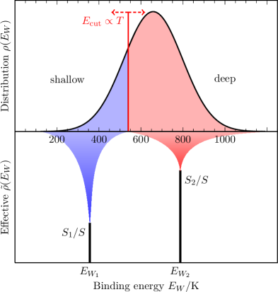
Figure 4: Basic idea of the mapping to the effective binary model.

4.2 Confirmation of mapping assumptions by simulations

The idea presented above has to be tested before we progress. To this end, we first introduce some additional notation and define the relevant quantities. We use subscripts $\omega$ for a realization of binding energies and $s$ for a single site. Then $E_{\omega,s}$ is the binding energy of site $s$ in realization $\omega$ (in this subsection, we will omit the subscript $W$ for brevity). Further, $r_{\omega,s}$ denotes the steady-state (or time-averaged) fraction of all reaction events in realization $\omega$ that takes place on site $s$; we call $r_{\omega,s}\in[0,1]$ the reactivity. We denote by $u_{\omega,s}$ the steady-state fraction of (physical) time that site $s$ in realization $\omega$ is occupied; $u_{\omega,s}\in[0,1]$ is called the occupancy.

We are interested in the relation between the binding energy of a certain site and its reactivity. On that account, we transform from the spatial distribution of reaction events to the distribution with respect to the local energy,

$$r_{\omega}(E)=\sum_{s}r_{\omega,s}\delta(E-E_{\omega,s}).$$ (9)

Obtained from a limited number of sites, $r_{\omega}(E)$ is obviously only a collection of $S$ sample values from an imagined smoothed function. Gathering information from a set $\{\omega\}$ of realizations, we additionally have to weight this distribution for each single realization $\omega$ according to the efficiency $\eta_{\omega}$ of the latter, effectively accounting for the number of reaction events during a certain period of time: A site with given energy might be responsible for a much larger fraction in one realization simply because in distant parts of the surface the particular energy landscape results in fewer events. In this case the overall efficiency of this particular realization will be diminished, and rescaling by the efficiency removes this unwanted distortion. The result (which we still call “reactivity”) reads

$$r_{\{\omega\}}(E)=\frac{\sum_{\omega}r_{\omega}(E)\cdot\eta_{\omega}}{\sum_{\omega}\eta_{\omega}},$$ (10)

including proper normalization

$$\sum_{E}r_{\{\omega\}}(E)=\frac{\sum_{\omega}\eta_{\omega}\sum_{s}r_{\omega,s}\sum_{E}\delta(E-E_{\omega,s})}{\sum_{\omega}\eta_{\omega}}=\frac{\sum_{\omega}\eta_{\omega}\left(\sum_{s}r_{\omega,s}\right)}{\sum_{\omega}\eta_{\omega}}=1.$$ (11)

The slightly clumsy notation is an artifact of the finite number of samples. In the limit considering the statistical ensemble of all possible realizations, the $E$ sum becomes an integral, and functions of $E$ become smooth.

For the occupancy of sites of a certain energy, we transform analogously to the above. Comprising several realizations does not need any weighting here, since the definition of the occupancy $u_{\omega,s}$ of a site does not relate to the total coverage in the realization. Normalization, however, implies we factor out the total number of particles in all realizations. Noting that the time-averaged total coverage in realization $\omega$ reads $N_{\omega}=\sum_{s}u_{\omega,s}$, we have

$$u_{\{\omega\}}(E)=\frac{\sum_{\omega}u_{\omega}(E)}{\sum_{\omega}N_{\omega}},$$ (12)

again called “occupancy”. Then

$$\sum_{E}u_{\{\omega\}}(E)=\frac{\sum_{\omega}\sum_{s}u_{\omega,s}\sum_{E}\delta(E-E_{\omega,s})}{\sum_{\omega}N_{\omega}}=\frac{\sum_{\omega}\left(\sum_{s}u_{\omega,s}\right)}{\sum_{\omega}N_{\omega}}=1.$$ (13)

Figure 5 shows the occupancy and the reactivity as functions of the binding energy, comprised from KMC simulations for $10$ realizations. We have chosen the paradigmatic example of the normal distribution here, with a relative width of $\tilde{\sigma}=30\%$, and for several temperatures. The unprocessed functions $u_{\{\omega\}}(E)$ and $r_{\{\omega\}}(E)$ are not shown, as they exhibit strong fluctuations (we return to this issue in section 4.6). Instead, we present better approximations of the smooth ensemble averages, which we denote by $u(E)$ and $r(E)$. These approximations are obtained by a sliding average, in which the function’s value at each sample energy $E$ is replaced by the average of all points within a certain energy neighborhood. This is preferable to an average over a fixed number of neighboring points, since samples are not equally spaced on the energy scale. In our plots we use an energy interval of $4\%$ of the total range of energies sampled. The original distribution of binding energies is drawn as a thin line for orientation. In order that the plots can be easily compared, we have rescaled this distribution to have a maximum value of unity. Likewise, we have rescaled $u(E)$ and $r(E)$ by a constant factor such that $u(E)$ attends a maximal value of unity as well.

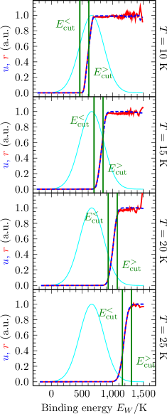
Figure 5: (Rescaled) occupancy $u(E_{W})$ (blue, dashed) and reactivity $r(E_{W})$ (red) versus binding energy $E_{W}$ of the sites, for the normal distribution of relative width $\tilde{\sigma}=30\%$ and at temperatures $T=10,\,15,\,\dots,\,25\ \mathrm{K}$ (top to bottom). The rescaled PDF (thin cyan line) is shown for reference. The vertical green lines mark two specific choices for $E_{\mathrm{cut}}$ to be defined in section 4.3.

Whenever sample-to-sample fluctuations become small, both occupancy and reactivity very clearly distinguish two types of sites according to their energy, with a fairly steep “step” between them. For lower energies there is little to no activity, and we identify these sites as effectively shallow. The sites with higher energies, however, provide nearly all the coverage and reaction events, and are effectively deep. Moreover on both sides of this border, the precise energy of the individual sites does no longer play any role.

The threshold energy $E_{\mathrm{cut}}$ separating both types of sites moves to higher energies as the temperature increases, as expected. For very high temperatures, only very few sites from the distribution tail still contribute coverage and reactions. On the other hand, we checked that the cut is largely independent of the shape and width of the distribution. Again, this is compatible with our earlier thoughts and will be substantiated in the next subsection. Figure 6 gives one example for the exponential and the uniform distribution, respectively, qualitatively similar to the results for the normal distribution. For the exponential distribution, high-energy tails decay more slowly than for the normal one, leading to a picture for $T=30\ \mathrm{K}$ which resembles those for lower temperatures in the normal-distribution case (with deep sites still over a large range of energies). The plot for the uniform distribution at $T=10\ \mathrm{K}$ hardly shows fluctuations in the (smoothed) occupancy and reactivity, compared with the normal distribution. This is due to the fact that there are no high-energy tails, so that energies are roughly equally (and “densely”) spaced up to their maximum, and hence few outliers do not affect the smoothed plot at all.

Lastly, we find the agreement between the graphs for occupancy and reactivity remarkable in all instances. This shows that exactly the highly-occupied sites are those on which reactions take place, just as in the genuinely binary model. Together we thus have numerical proof of the arguments we have presented in section 4.1.

  

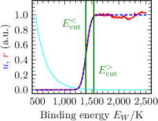
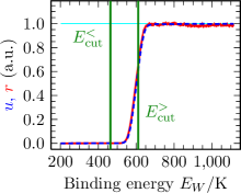
Figure 6: As in figure 5, $u(E_{W})$ (blue, dashed) and $r(E_{W})$ (red), for an exponential distribution with $\tilde{\sigma}=30\%$ at $T=30\ \mathrm{K}$ (left), and for a uniform distribution with $\tilde{\sigma}=40\%$ at $T=10\ \mathrm{K}$ (right). Rescaled PDF’s (thin cyan line) shown for reference.

4.3 Heuristic derivation of the mapping

There are a multitude of strategies to arrive at a mapping from the continuous to the binary model. We should state very clearly that, in fact, one could even (implicitly) define an effective homogeneous model which uses only one type of site. Since a homogeneous system can exhibit the whole range of values $[0,1]$ of the efficiency $\eta$, it is mathematically trivial that, if we may choose all parameters appropriately, it can reproduce the efficiency found in the continuous model. Apart from the implicitness of such a definition, this does not lead to any understanding of the underlying physics, however.

Our approach is different. We try to retain as many features of the continuous-distribution model as possible, altering only a minimal subset of parameters—this way, we minimize the arbitrariness of the mapping. The physically plausible strategy is to restrict changes to the binding energy distribution itself; we will find an equivalent system where only the “well depths” of sites are changed (to a binary distribution). Concretely, this implies that we keep $f$, $T$, $S$ and $\nu$ fixed.

Note that we speak of a mapping of the binding energies $E_{W}$ throughout, but the hopping barriers $E_{a}$ are of similar importance. In the continuous case they are fixed by demanding constant $\Delta E=E_{W}-E_{a}$ for all sites, which guarantees detailed balance, and implies a constant ratio $W/a$. We stick to this choice (particularly for the detailed-balance argument), using the same $\Delta E$ for the binary distribution.

Consequently, there are three quantities left that define the mapping: the discrete binding energies $E_{W_{1}}$ and $E_{W_{2}}$ of shallow and deep sites in the effective model, respectively, and the number of both types of sites, conveniently parametrized by a cutting energy $E_{\mathrm{cut}}$ at which we split the distribution of binding energies.

The discrete binary distribution has to capture the essential features of the original continuous one. The two most obvious properties are the mean binding energy $\langle E_{W}\rangle$ and the standard deviation $\sigma$. We demand that the effective binary distribution has the same mean and standard deviation. Given the number of shallow and deep sites, $S_{1}$ and $S_{2}$, this fixes the discrete binding energies to read

$$E_{W_{1}}=\langle E_{W}\rangle-\sigma\sqrt{S_{2}/S_{1}},\qquad E_{W_{2}}=\langle E_{W}\rangle+\sigma\sqrt{S_{1}/S_{2}}.$$ (14)

Recall our earlier assumption that both $S_{1}$ and $S_{2}$ are not too small, and in particular that the binary model does not degenerate to a homogeneous model in the regime of our interest.

It only remains to choose $E_{\mathrm{cut}}$, which governs how many sites are regarded as shallow and deep. As the simplest choice, we assume that this energy is independent of the shape and parameters of the distribution.

Now consider the limiting regime of high temperature. There are many shallow and few deep sites, regardless of the precise form of $E_{\mathrm{cut}}$. The limiting factor for the efficiency is lack of coverage on the deep sites, while mobility on shallow sites (to quickly funnel atoms to the deep ones) is a given. Hence, we have to split the binding energy distribution at an $E_{\mathrm{cut}}$ such that at this and at higher energies, sites are sufficiently occupied. This energy is set by $f=\left.W\right\rvert_{E_{W}=E_{\mathrm{cut}}}$, such that without any reactions, we would have half-filling on average. This means

$$E_{\mathrm{cut}}=E_{\mathrm{cut}}^{<}:=T\ln(\nu/f)\quad\text{(high $T$)}.$$ (15)

Mobility on the shallow sites is then guaranteed by $\left.a\right\rvert_{E_{W}\leq E_{\mathrm{cut}}}\geq\left.a\right\rvert_{E_{W}=E_{\mathrm{cut}}}\gg\left.W\right\rvert_{E_{W}=E_{\mathrm{cut}}}=f$.

For low temperatures, on the other hand, the overall coverage is high, and there are few shallow but lots of deep sites. In this regime the efficiency is not limited by lack of coverage, but by a lack of mobility on the shallow sites. Particles have to be able to hop at least as frequently as new ones arrive, or else LH rejection will curtail the efficiency. Therefore, the maximal energy of “working” shallow sites is set by $f=\left.a\right\rvert_{E_{W}=E_{\mathrm{cut}}}$, and sites at lower energies have $a>f$. Re-writing the condition using $E_{a}=E_{W}-\Delta E$ we obtain

$$E_{\mathrm{cut}}=E_{\mathrm{cut}}^{>}:=T\ln(\nu/f)+\Delta E\quad\text{(low $T$)}.$$ (16)

On the deep sites, we then have $f\geq\left.a\right\rvert_{E_{W}\geq E_{\mathrm{cut}}}\gg W$, so high coverage there is guaranteed.

These choices for $E_{\mathrm{cut}}$ are shown as vertical lines in the energy-resolved pictures for occupancy and reactivity, figure 5 and figure 6. On the other hand, the latter quantities suggest a reasonable choice for $E_{\mathrm{cut}}$ themselves, say, the energy at which occupancy and reactivity reach half of their maximal value. Comparing these choices, $E_{\mathrm{cut}}$ as suggested by the plots is always found between $E_{\mathrm{cut}}^{<}$ and $E_{\mathrm{cut}}^{>}$ (as defined above). For low temperatures the suggested cutting energy indeed moves closer to the upper energy $E_{\mathrm{cut}}^{>}$, whereas with increasing temperature it comes ever closer to the lower energy $E_{\mathrm{cut}}^{<}$. Our heuristic derivation of the threshold energy is hence confirmed by numerical simulations.

The shift of $\Delta E$ between the two choices reflects the fact that in the above arguments, for high temperatures the distribution of binding energies is cut in two, while at low temperatures the distribution of diffusion barriers is cut. These results are indeed independent of the shape, mean, and width of the distribution, as suggested above. The limiting temperature regimes correspond to finite temperatures (not to $T\to 0$ and $T\to\infty$, that is), hence the transition between them involves additional temperature scales (describing location and width). These quantities evidently have to depend on the shape and width of the distribution, which we will confirm by simulation results (see below). We have not found a convincing theoretical argument to determine these scales. In practice, it is still straightforward to determine the appropriate choice for $E_{\mathrm{cut}}$. Sites with energies in the range $[E_{\mathrm{cut}}^{<},E_{\mathrm{cut}}^{>}]$ provide coverage and mobility, and could be labeled either deep or shallow, depending on this choice. The proper choice of $E_{\mathrm{cut}}$ in the limits of low and high temperature regards these sites to provide the scarce property which limits the efficiency, respectively. The “opposite” choice misinterprets their role and leads to substantially lower efficiency. Summing up, in both limits, one chooses $E_{\mathrm{cut}}$ such that it leads to the highest possible efficiency in the effective model. It is then plausible to stick with this prescription for intermediate temperatures as well.

In principle, cutting the distribution at $E_{\mathrm{cut}}$ provides real values for the numbers $S_{i}$ of sites of a given type. To stay true to the idea that we replace the whole energy landscape by an effective one, we round to the nearest integer values for $S_{i}$, when the effective system has physically sensible parameters throughout. In the case where the system is sufficiently large and still has a substantial number of both shallow as well as deep sites, the difference to the nearest integer values is negligible anyway.

4.4 Comparison to KMC simulations

We have introduced the mapping to an effective binary model, and we have reviewed earlier (cf. section 3.2) how this model is described and solved using rate equations. We will now compare its predictions with the outcome of KMC simulations. For each temperature and distribution shape and width, we simulated 10 realizations as described in section 2.2. Figure 7 shows that overall, agreement between the KMC results and the prediction of the effective model is very good, for both the coverage and the efficiency. Most importantly, the temperature range of efficient reaction is reproduced with very good accuracy in most circumstances—this is the truly valuable information, compared with minor deviations in the efficiency itself. There is some discrepancy between KMC and effective model results in the high-temperature tail for the normal and the exponential distribution. The rate equation solution of the effective model describes hops between any two sites of the lattice, such that spatial correlations are switched off entirely. If we include such “long hops” in the KMC simulations, the efficiency also increases (as checked in several test runs, and as previously found and explained for the binary system [18]), and it then agrees even better with the effective model results.

The system now shows a broad temperature window of high efficiency, different from the homogeneous system, but also from the binary case, as far as the slow decay to higher temperatures is concerned (cf. figure 3). Likewise, we observe a smooth monotonic transition from full coverage to an empty system, in stark contrast to the binary case—this illustrates once more that the effective binary model we map to changes its structure with temperature. It is also evident that sample-to-sample fluctuations are a subordinate effect throughout, even on the critical flanks of the efficiency and for the long-tailed exponential distribution. We will return to this issue in section 4.6.

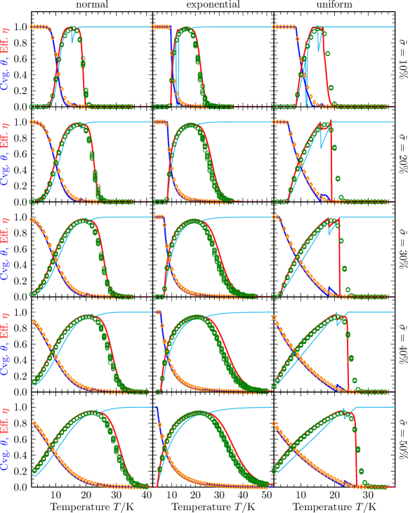
Figure 7: Coverage $\theta$ (orange diamonds, blue lines) and efficiency $\eta$ (green circles, red lines) versus temperature $T$, of the continuous-distribution system from KMC simulations (marks, one per realization), and as obtained for the effective binary model via rate equations (lines). Also shown is the fraction $S_{1}/S$ of shallow sites in the effective model (thin cyan line). Columns (left to right) for normal, exponential, and uniform distribution, rows for several relative widths $\tilde{\sigma}=\sigma/\langle E_{W}\rangle$ as indicated. The spikes seen at an intermediate temperature, most notably for $S_{1}/S$, are a result of the switch of $E_{\mathrm{cut}}$ between $E_{\mathrm{cut}}^{>}$ and $E_{\mathrm{cut}}^{<}$.

Of special interest is the range of validity of the mapping idea. As emphasized before, it relies on the presence of both types of sites, shallow and deep, in the effective model. This is no longer satisfied at very low temperatures, when all sites are effectively deep ($S_{1}=0$), and at very high temperatures, when all sites are effectively shallow ($S_{2}=0$). Obviously, these limits are reached at less extreme temperatures for narrower distributions (upper rows), and in the absence of distribution tails, as exemplified by the uniform and (to lower energies) the exponential distribution. The effective model degenerates to a homogeneous system then, with the binding energy given by the mean of the distribution. For the figure, we correspondingly replaced the numerical solution of the effective binary model by the analytical results for the homogeneous case.

For very low temperatures, the examples studied here show essentially full coverage and zero efficiency, which is trivially reproduced by the homogeneous rate equation results. The support of the exponential and the uniform distribution is bounded to low energies. Therefore, the transition to the $S_{1}=0$ regime is not smooth, which manifests itself in the discontinuous derivative of coverage and efficiency. For high temperatures, the situation is more subtle. The normal and the exponential distribution, which both have tails to high energies, are still accurately described at very high temperatures: For most of the panels shown, $S_{2}=0$ is reached eventually, but only after the KMC efficiency has vanished completely. Up to this temperature, there are still some deep sites in the effective model owed to the distribution tail (not visible in the plots due to limited resolution), and they are sufficient to reproduce KMC results. At still higher temperatures, the effective homogeneous system trivially reproduces zero coverage and efficiency. For the uniform distribution, however, KMC results show a fast (but by no means abrupt) decay of the efficiency with increasing temperature. Due to the lack of high-energy tails (which could still provide a few deep sites), the effective model now degenerates ($S_{2}=0$) at a temperature low enough that KMC results still exhibit some efficiency. For a very narrow distribution ($\tilde{\sigma}=10\%$) this happens so early ($T\approx 18\ \mathrm{K}$) that the resulting effective model (homogeneous with binding energy $\langle E_{W}\rangle$) still shows the high-temperature flank seen in figure 2. For all wider distributions the switch to the degenerate effective model occurs at temperatures where the homogeneous system has no efficiency left, while the KMC results still have residual efficiency, most likely due to the mere fact that there is a distribution of different binding energies (in part exceeding $\langle E_{W}\rangle$) and possibly some spatial correlations.

4.5 Tail shape and analytical expressions

For a homogeneous system, the tail shape of the efficiency $\eta(T)$ (fairly symmetric to low and high temperatures) is well understood (cf. section 3.1): The efficiency decays exponentially with the temperature in both cases, since all rates are thermally activated. From the rate equation efficiency (3) one finds

$$\eta\simeq 2\frac{a}{f}=2\frac{\nu}{f}\rme^{-E_{a}/T}\quad\text{(low-$T$ tail)},\qquad\eta\simeq 2\frac{fa}{W^{2}}=2\frac{f}{\nu}\rme^{(2E_{W}-E_{a})/T}\quad\text{(high-$T$ tail)},$$ (17)

which mirrors the temperature bounds (4) and (5). The tail shapes for the binary system are the same as for the homogeneous system, since for each tail only reaction on one type of site is important.

For continuously distributed binding energies, however, the situation is different. There are many similar binding energies acting almost but not exactly the same (at a certain temperature). This is reflected by the slower decay of the efficiency. We now use the mapping to the effective binary model to derive an analytical expression for the (low-temperature) tail shape.

As alluded to in section 3.1, the binary system exhibits a plateau of the efficiency $\eta(T)$ between the two peaks of the corresponding homogeneous systems in certain conditions. More precisely, one needs enough deep binding sites—depending on the temperature, flux and the difference in the binding energies of the two types of sites. Following [18], we let $T^{\mathrm{eq}}$ denote the temperature below which the random walk length (on shallow sites), $\ell_{\mathrm{rw}}=\sqrt{a_{1}/W_{1}}$, exceeds the average hopping length before encountering a trap [35, 36], $\ell_{\mathrm{trap}}\simeq\sqrt{S/(\pi S_{2})\cdot\ln S}$: At lower temperatures, particles typically end in deep sites. If $T^{\mathrm{eq}}>T_{2}^{\mathrm{max}}$ we find a plateau, with an efficiency of [18]

$$\eta_{\mathrm{p}}\approx\frac{2}{1+S/S_{1}}.$$ (18)

Now in the effective binary model, the energies and numbers of both types of sites are functions of $E_{\mathrm{cut}}$ and thus depend on the temperature $T$. For the low temperature tail of all shown distributions, we have sufficiently many deep sites $S_{2}$ in the effective model, such that the condition $T^{\mathrm{eq}}>T_{2}^{\mathrm{max}}$ is satisfied—the effective model (for the given temperature) features a plateau. One also finds that $T_{1}^{\mathrm{max}}<T<T_{2}^{\mathrm{max}}$, such that we evaluate the model on this plateau, and the formula (18) applies. The fraction of shallow sites $S_{1}/S$ in the effective model is given by the cumulative distribution function $\Phi(E_{\mathrm{cut}}):=\int_{-\infty}^{E_{\mathrm{cut}}}\rho(E_{W})\,\mathrm{d}E_{W}$. Lastly, since we are in the low-temperature tail, we have (cf. section 4.3) $E_{\mathrm{cut}}=E_{\mathrm{cut}}^{>}=T\ln(\nu/f)+\Delta E$, leading to

$$\eta\approx\frac{2}{1+\Phi(T\ln(\nu/f)+\Delta E)^{-1}}\quad\text{(low $T$)}.$$ (19)

This expression shows a much weaker dependence on temperature compared with the homogeneous and (genuinely) binary cases with their exponential decay. It also explains that the broader tails of the efficiency do not necessarily originate from tails of the underlying distribution $\rho(E_{W})$ (provided there still are both deep and shallow sites). Rather, the decisive factor is that the mapping introduces a $T$-dependent split into shallow and deep sites via the cutting energy $E_{\mathrm{cut}}$—without thermally activated rates playing any role. Moreover, this implies a lower temperature bound of efficient reaction (where $\eta=1/2$) given by

$$\Phi(T^{\mathrm{low}}\ln(\nu/f)+\Delta E)=\frac{1}{3}.$$ (20)

Figure 8 shows that indeed the low-temperature expression (19) is extremely accurate up to intermediate temperatures around the efficiency peak temperature. This corresponds to the fact that the plateau in the binary model breaks down only at rather low fraction $S_{2}/S$ (depending on $E_{W_{2}}-E_{W_{1}}$). We have checked that these statements hold true for all parameters used in figure 7.

  

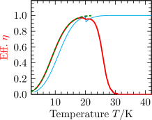
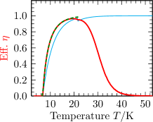
Figure 8: Efficiency $\eta$ versus temperature $T$ in the effective binary model, evaluated using the numerical solution of rate equations (red, as in figure 7) and as given by the analytical expression (19) (green, dashed), for a normal distribution with $\tilde{\sigma}=30\%$ (left), and for an exponential distribution with $\tilde{\sigma}=30\%$ (right). For reference, the fraction $S_{1}/S$ of shallow sites in the effective model is shown again (thin cyan line).

For the high-temperature tail, the situation is more subtle. Here, the effective binary model only has few deep sites, and they are far from the mean energy $\langle E_{W}\rangle$ (cf. (14)). Even a fixed such model has no efficiency plateau then, but a $T$-dependent efficiency drop between the “homogeneous peaks” [18, Figure 5]. We do not have an illuminating analytical expression for this dependence, wherefore the upper temperature bound $T^{\mathrm{up}}$ remains inaccessible as well.

4.6 Realization dependence

We first comment on the effect of the quenched nature of disorder at the microscopic level. In any particular realization of the system, sites with similar binding energy may live in a very different local neighborhood. Therefore, they can differ strongly in the occupancy $u$ and the reactivity $r$. This is very prominent in the raw simulation data, and the variability was intentionally reduced in figure 5 and figure 6 by using a sliding average. The site-to-site variability only vanishes in passing to the ensemble of all realizations (or infinite system size $S\to\infty$), whereas purely stochastic fluctuations decrease with increasing simulation time. We have confirmed this distinction by comparison with KMC simulations in which spatial correlations are suppressed (“long hops” between all sites are included, cf. section 4.4). This indeed removes the major part of the variability in occupancy and reactivity.

Interestingly, site-to-site variations are much more pronounced for the reactivity than for the occupancy. The reason for this is as follows: Consider the system dynamics over a certain period of time, and we are only concerned with effectively deep sites, where essentially all coverage and reaction events are concentrated. The number of such events on a given site is (to a good approximation) Poisson-distributed, with a rate parameter depending on the local surroundings. Together with statistical fluctuations, this gives rise to the variability seen in the reactivity $r$. For the occupancy $u$, individual occupation times of a site are added up and compared with the total time passed. Since only a reaction event empties the site (hopping and desorption from deep sites is negligible), there are as many individual occupation times as there are reaction events on this site. This strongly anticorrelates the number of such events with the length of individual occupation times—if particles arrive more frequently, single occupation times are shorter. Therefore the number of reaction events (and hence, the reactivity) can strongly differ between two sites of similar energy, yet the fraction of time they are occupied (the occupancy) will differ far less. Note that the reduced variability in the occupancy versus the reactivity immediately translates to that of the total coverage versus the efficiency between different realizations.

We now turn to this dependence of global quantities on the realization. The overall system size in this article is large enough not to expect a noticeable dependence of the coverage and the efficiency on the realization. This is confirmed in figure 7 for the lower-temperature regime of both the coverage and the efficiency. For the high-temperature decay of the efficiency, however, such a dependence is clearly seen in the vertical spread of symbols referring to different realizations, both in the case of the normal and the exponential distribution. Somewhat counterintuitively, the variability between realizations decreases with increasing disorder strength (width of the distribution).

The mapping to an effective model explains if and why we see significant sample-to-sample variations of the efficiency. As explained at the end of section 4.5, for high temperatures the effective binary model has few deep sites, far from the mean binding energy. We know (from both simulations and numerical solutions of the rate equations), that in this regime the efficiency of the binary system is very sensitive to the exact number of deep sites [18]. This is perfectly intuitive, since there are so few of them, yet they are very important for the reaction. Applying the mapping to different realizations of the finite continuous-distribution system, the number of effectively deep sites also varies, and because there are few in any case, the variations relatively matter a lot. The sensitivity of the effective binary model to their number (at fixed $T$) thus explains the realization dependence of the KMC efficiency of the continuous system (figure 7), and why it only shows on the high-temperature flank. Moreover, it is more pronounced for narrower distributions of the binding energy, since steeper flanks of the PDF lead to larger relative variations in the small number of effectively deep sites. The coverage is already very small in this regime, such that its realization dependence is not visible in figure 7.

It is an interesting feature that, though part of a nominally large system, the smallness of one crucial component (the number of deep sites) is enough to imply a strong realization dependence of a key quantity such as the efficiency. This constitutes an effective small-system regime, in the sense that the realization dependence will still vanish as usual upon increasing the total system size $S$. In this context, the mapping to an effective model concisely explains that depending on the temperature, we are in different regimes as to the effect of disorder. The asymmetry between shallow and deep sites (i.e., why is there no strong sensitivity when there are only few of the former?) is easily resolved. At temperatures so low that there are very few effectively shallow sites only, $S_{1}/S\ll 1$, application of the plateau formula (18) (as justified in section 4.5) yields $\eta_{\mathrm{p}}\approx 2S_{1}/S\ll 1$. Therefore, whatever sample-to-sample variability there is in the efficiency cannot be seen in figure 7. On the other hand, the sensitivity of the coverage to the realization is much weaker anyway, as shown above.

5 Conclusions

We have studied the steady state of a two-dimensional diffusion-limited reaction model, with disordered binding energies drawn from a continuous distribution. Sites in this model play one of two distinct roles, as we have verified in simulations: If the binding energy is low enough, sites provide mobility of particles to traverse the surface. If their binding energy is strong enough, they instead provide coverage by trapping particles for a long time. As a result, we can map the continuous-distribution model to an effective binary model of these shallow and deep sites, which is well understood and easily solved. The precise form of the mapping has been derived heuristically and does not depend on any fitting parameters. The model yields results for the coverage and the reaction efficiency which are in good agreement with simulations. Compared with the case of discrete distributions studied before, the model shows a markedly different behavior, with the temperature range of efficient reaction broadened and the tails decaying much slower. The mapping explains this slower decay for low temperatures, as well as the sample-to-sample fluctuations found for the high-temperature decay of the reaction efficiency.

As discussed in the introduction, the particular model studied here is paradigmatic for applications in astrophysics and in heterogeneous surface catalysis. Moreover, the existence of a simple mapping from a highly complex to a simple effective model is of great theoretical value. The explanations we provide in terms of microscopic processes can hopefully serve as a recipe to find similar relations for other types of disordered systems.

References

References

- [1] ben-Avraham D and Havlin S 2000 Diffusion and Reactions in Fractals and Disordered Systems (Cambridge University Press)
- [2] Haus J W and Kehr K W 1987 Phys. Rep. 150 263–406
- [3] Bouchaud J P and Georges A 1990 Phys. Rep. 195 127–293
- [4] Zel’dovich Y B, Molchanov S A, Ruzmaĭkin A A and Sokolov D D 1987 Sov. Phys. Usp. 30 353–369
- [5] Gärtner J and den Hollander F 2006 Ann. Probab. 34 2219–2287
- [6] Zhdanov V P 2002 Surf. Sci. Rep. 45 231–326 ISSN 0167-5729
- [7] Frachebourg L, Krapivsky P L and Redner S 1995 Phys. Rev. Lett. 75 2891–2894
- [8] Head D A and Rodgers G J 1996 Phys. Rev. E 54 1101–1105
- [9] Oshanin G, Popescu M N and Dietrich S 2004 Phys. Rev. Lett. 93 020602
- [10] Herbst E, Chang Q and Cuppen H M 2005 J. Phys.: Conf. Ser. 6 18–35
- [11] Gould R J and Salpeter E E 1963 Astrophys. J. 138 393–407
- [12] Hollenbach D and Salpeter E E 1971 Astrophys. J. 163 155–164
- [13] Green N J B, Toniazzo T, Pilling M J, Ruffle D P, Bell N and Hartquist T W 2001 Astron. Astrophys. 375 1111–1119
- [14] Biham O and Lipshtat A 2002 Phys. Rev. E 66 056103
- [15] Lohmar I and Krug J 2006 Mon. Not. Roy. Astron. Soc. 370 1025–1033
- [16] Lohmar I and Krug J 2009 J. Stat. Phys. 134 307
- [17] Lohmar I, Krug J and Biham O 2009 Astron. Astrophys. 504 L5–8
- [18] Wolff A, Lohmar I, Krug J, Frank Y and Biham O 2010 Phys. Rev. E 81 061109
- [19] Imry Y and Ma S k 1975 Phys. Rev. Lett. 35 1399–1401
- [20] Nattermann T 1998 Theory of the random field Ising model Spin Glasses and Random Fields (Directions in Condensed Matter Physics no 12) ed Young A P (Singapore: World Scientific)
- [21] Swift M R, Bray A J, Maritan A, Cieplak M and Banavar J R 1997 Europhys. Lett. 38 273–278
- [22] Fytas N G, Malakis A and Eftaxias K 2008 J. Stat. Mech.: Theor. Exp. 2008 P03015
- [23] Luck J M and Nieuwenhuizen T M 1988 J. Stat. Phys. 52 1–22
- [24] Langmuir I 1918 J. Am. Chem. Soc. 40 1361–1403
- [25] Voter A F 2007 Introduction to the kinetic monte carlo method Radiation Effects in Solids (Nato Science Series II: Mathematics, Physics And Chemistry vol 235) ed Sickafus K E, Kotomin E A and Uberuaga B P (Springer) URL http://www.ipam.ucla.edu/publications/matut/matut_5898_prepri%%****␣paper.bbl␣Line␣100␣****nt.pdf
- [26] Montroll E W and Weiss G H 1965 J. Math. Phys. 6 167
- [27] Biham O, Furman I, Pirronello V and Vidali G 2001 Astrophys. J. 553 595–603
- [28] Katz N, Furman I, Biham O, Pirronello V and Vidali G 1999 Astrophys. J. 522 305–312
- [29] Chang Q, Cuppen H M and Herbst E 2005 Astron. Astrophys. 434 599–611
- [30] Herbst E and Cuppen H M 2006 PNAS 103 12257–12262
- [31] Tielens A G G M 1995 Talk at a conference on interstellar chemistry in Leiden, The Netherlands
- [32] Krug J 2003 Phys. Rev. E 67 065102(R)
- [33] Biham O, Krug J, Lipshtat A and Michely T 2005 Small 1 502–504
- [34] Lederhendler A and Biham O 2008 Phys. Rev. E 78 041105
- [35] Montroll E W 1969 J. Math. Phys. 10 753
- [36] Evans J W and Nord R S 1985 Phys. Rev. A 32 2926–2943