Collective strong coupling between ion Coulomb crystals and an optical cavity field:
Theory and experiment

Abstract

A detailed description and theoretical analysis of experiments achieving coherent coupling between an ion Coulomb crystal and an optical cavity field are presented. The various methods used to measure the coherent coupling rate between large ion Coulomb crystals in a linear quadrupole radiofrequency ion trap and a single-field mode of a moderately high-finesse cavity are described in detail. Theoretical models based on a semiclassical approach are applied in assessment of the experimental results of [P. F. Herskind et al., Nature Phys. 5, 494 (2009)] and of complementary new measurements. Generally, a very good agreement between theory and experiments is obtained.

I Introduction

Cavity Quantum Electrodynamics (CQED) constitutes a fundamental platform for studying the quantum dynamics of matter systems interacting with electromagnetic fields Berman1994 ; Haroche2006 . For a single two-level quantum system interacting with a single mode of the electromagnetic field of a resonator, a particularly interesting regime of CQED is reached when the rate, $g$, at which single excitations are coherently exchanged between the two-level system and the cavity field mode exceeds both the decay rate of the two-level system, $\gamma$, and the rate, $\kappa$, at which the cavity field decays Rempe1994Cavity . This so-called strong coupling regime was investigated first with single atoms in microwave and optical cavities Brune1996 ; Thompson1992Observation and recently with quantum dots Badolato2005Deterministic ; khitrova2006 and superconducting Josephson junctions wallraff2004 ; Chiorescu2004Coherent . In the optical domain, the use of ultrahigh-finesse cavities with a very small modevolume allows for reaching the confinement of the light field required to achieve strong coupling with single neutral atoms Hood1998 ; Rempe1994Cavity ; Maunz2005 . With charged particles, however, the insertion of dielectric mirrors in the trapping region makes it extremely challenging to obtain sufficiently small cavity modevolumes, due to the associated perturbation of the trapping potentials and charging effects Harlander2010Trapped-ion ; Herskind2011AMicrofabricated . Although the strong coupling regime has not yet been reached with ions, single ions in optical cavities have been successfully used for, e.g., probing the spatial structure of cavity fields Guthohrlein2001AsingleIon , enhanced spectroscopy Kreuter2004 , the generation of single photons Keller2004Continuous ; Barros2009Deterministic , the investigation of cavity sideband cooling Leibrandt2009Cavity , or the demonstration of a single ion laser Dubin2010Quantum .

For an ensemble of $N$ identical two-level systems simultaneously interacting with a single mode of the electromagnetic field, the coherent coupling rate is enhanced by a factor $\sqrt{N}$ Haroche2006 . This leads to another interesting regime of CQED, the so-called collective strong coupling regime Haroche2006 , where the collective coupling rate $g_{\mathrm{N}}=g\sqrt{N}$ is larger than both $\kappa$ and $\gamma$. This regime, first explored with Rydberg atoms in microwave cavities Kaluzny1983 , has been realized in the optical domain with atomic beams Thompson1992Observation , atoms in magneto-optical traps Lambrecht1996 ; Nagorny2003Collective ; Chan2003Observation ; Kruse2004Observation ; Chen2011Conditional , Bose-Einstein condensates Brennecke2007Cavity ; Colombe2007Strong , and, recently, with ion Coulomb crystals Herskind2009Realization . This cavity-enhanced collective interaction with an ensemble has many applications within quantum optics and quantum information processing Kimble2008 , including the establishment of strong nonlinearities Lambrecht1995Optical ; Joshi2003Optical , QND measurements Grangier1991Observation ; Roch1997Quantum ; Mielke1998Nonclassical , the production Black2005On-Demand ; Thompson2006AHigh-Brightness and storage Simon2007 ; Tanji2009Heralded of single-photons, the generation of squeezed and entangled states of light Lambrecht1996 ; Josse2003Polarization ; Josse2004Continuous and atoms Leroux2010Implementation ; Chen2011Conditional , the observation of cavity optomechanical effects Nagorny2003Collective ; Kruse2004Observation ; Klinner2006Normal ; Slama2007Superradiant ; Murch2008Observation ; Brennecke2008 , cavity cooling Chan2003Observation ; Black2003Observation , and the investigation of quantum phase transitions Baumann2010Dicke .

This paper provides a detailed description and a theoretical analysis of experiments achieving collective strong coupling with ions Herskind2009Realization . The various methods used to measure the coherent coupling rate between large ion Coulomb crystals in a linear quadrupole radiofrequency ion trap and a single field mode of a moderately high-finesse cavity ($\mathcal{F}\sim 3000$) are described in detail. Theoretical models based on a semiclassical approach are applied in assessment of the experimental results of Ref. Herskind2009Realization as well as of complementary new measurements. Generally, a very good agreement between the theoretical predictions and the experimental results is obtained. As also emphasized in Ref. Herskind2009Realization , the realization of collective strong coupling with ion crystals is important for ion-based CQED Lange2009CavityQED and enables, e.g., for the realization of quantum information processing devices, such as high-efficiency, long-lived quantum memories Lukin2000 ; Simon2007 and repeaters Duan2001 . In addition to the well-established attractive properties of cold, trapped ions for quantum information processing Leibfried2003Quantum ; Blatt2008Entangled , ion Coulomb crystals benefit from unique properties which can be exploited for CQED purposes. First, their uniform density under linear quadrupole trapping conditions Drewsen1998 ; Hornekaer2002Formation ; Hornekaer2001 makes it possible to couple the same ensemble equally to different transverse cavity modes Dantan2009Large and opens for the realization of multimode quantum light-matter interfaces Lvovsky2009Optical , where the spatial degrees of freedom of light can be exploited in addition to the traditional polarization and frequency encodings Vasilyev2008Quantum ; Tordrup2008Holographic ; Wesenberg2011Dynamics . Second, their cold, solid-like nature combined with their strong optical response to radiation pressure forces and their tunable mode spectrum Dubin1991Theory ; Dubin1996Normal ; Dantan2010Non-invasive make ion Coulomb crystals a unique medium to investigate cavity optomechanical effects Kippenberg2008 . Ion Coulomb crystals could, for instance, be used as a model system to study the back action of the cavity light field on the collective motion of mesoscopic objects at the quantum limit, as was recently demonstrated with ultracold atoms Murch2008Observation ; Brennecke2008 ; Baumann2010Dicke . In addition, novel classical and quantum phase transitions could be investigated using cold ion Coulomb crystals in optical cavities Garcia-Mata2007Frenkel-Kontorova ; Retzker2008Double ; Fishman2008Structural ; Harkonen2009Dicke .

The paper is organized as follows: Sec. II presents the theoretical basis for the CQED interaction of ion Coulomb crystals and an optical cavity field. The cavity field reflectivity spectra, and the effective number of ions interacting with the cavity field are derived and the effect of temperature on the collective coupling rate is discussed. In Sec. III the experimental setup and the measurement procedures are described. Section IV presents various collective coupling rate measurements and compares them to the theoretical expectations. Section V shows measurements of the coherence time of collective coherences between Zeeman sublevels. A conclusion is given in Sec. VI.

II CQED interaction: theoretical basis

II.1 Hamiltonian and evolution equations

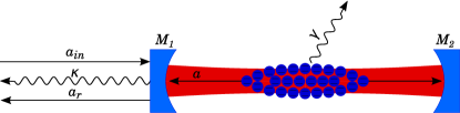
Figure 1: Scheme considered for the description of the interaction between an ion Coulomb crystals and the cavity field. The cavity is formed by the two mirrors ${M}_{1}$ and ${M}_{2}$. $a_{\mathrm{in}}$ is the input light field, $a$ the intracavity field, and $a_{\mathrm{r}}$ is the reflected field. $\kappa$ denotes the cavity field decay rate. The spontaneous dipole decay rate of the ions is denoted by $\gamma$.

We consider the interaction of $N_{\mathrm{tot}}$ two-level ions in a Coulomb crystal with a single mode of the electromagnetic field of an optical cavity (denoted by $\mathrm{nm}$), as depicted in Fig. 1. The single-ended linear cavity is formed by two mirrors M₁ (partial transmitter, PT) and M₂ (high reflector, HR) with intensity transmission coefficients $T_{1}$ and $T_{2}$ ($T_{1}\gg T_{2}$). The absorption loss coefficient per round-trip is $\mathcal{L}$ and the empty cavity field round-trip time is $\tau=2l/c$, where $l$ is the cavity length and $c$ the speed of light. The intracavity, input and reflected fields are denoted by $a$, $a_{\mathrm{in}}$, and $a_{\mathrm{r}}$, respectively. The interaction of an ensemble of $N$ identical two-level ions with a single mode of the cavity field can be described by a Jaynes-Cummings Hamiltonian of the form Haroche2006 ; Breuer2007TheTheory

$$H=H_{\mathrm{at}}+H_{\mathrm{l}}+H_{\mathrm{al}}$$ (1)

where, in the frame rotating at the laser frequency $\omega_{\mathrm{l}}$, the atom and light Hamiltonians are given by $H_{\mathrm{at}}=\hbar\Delta\sum_{j=1}^{N_{\mathrm{tot}}}\hat{\pi}_{j}^{(e)}$ and $H_{\mathrm{l}}=\hbar\Delta_{\mathrm{c}}\hat{a}^{\dagger}\hat{a}$. The atomic and cavity detunings are denoted by $\Delta=\omega_{\mathrm{at}}-\omega_{\mathrm{l}}$ and $\Delta_{\mathrm{c}}=\omega_{\mathrm{c}}-\omega_{\mathrm{l}}$, where $\omega_{\mathrm{at}}$ and $\omega_{\mathrm{c}}$ are the atomic and cavity resonance frequencies, respectively. $\hat{\pi}_{j}^{(e)}$ is the excited state population operator of the $j$-th ion and $\hat{a}$, $\hat{a}^{\dagger}$ are the intracavity field annihilation and creation operators. In the rotating wave approximation the interaction Hamiltonian reads

$$H_{\mathrm{al}}=-\hbar g\sum_{j=1}^{N_{\mathrm{tot}}}\Psi_{\mathrm{nm}}(\bm{r}_{j})(\hat{\sigma}_{j}^{\dagger}\hat{a}+\hat{\sigma}_{j}\hat{a}^{\dagger}).$$ (2)

where $\hat{\sigma}_{j}^{\dagger}$ and $\hat{\sigma}_{j}$ are the atomic rising and lowering operators, defined in the frame rotating at the laser frequency. The single-ion coupling rate $g$ is defined as $g=\mu_{\mathrm{ge}}E_{0}/\hbar$, where $\mu_{\mathrm{ge}}$ is the dipole element of the transition considered and $E_{0}$ the maximum electric field amplitude. The field distribution $E_{0}\Psi_{\mathrm{nm}}(\bm{r}_{j})$ is assumed to be that of a single-cavity Hermite-Gauss mode Kogelnik1966Laser . In the following, we will restrict ourselves to the fundamental $\mathrm{TEM}_{00}$ mode of the cavity and refer to Ref. Dantan2009Large for the coupling of ion Coulomb crystals to higher-order cavity transverse modes.

The coupled atom-cavity system is subject to decoherence, mainly through the spontaneous decay of the ions from the excited state and through the decay of the cavity field due to the finite reflectivity of the cavity mirrors and due to intracavity losses. These dissipative processes are characterized by the atomic dipole decay rate, $\gamma$, and by the total cavity field decay rate, $\kappa$, respectively. The cavity field decay rate is given by $\kappa=\kappa_{1}+\kappa_{2}+\kappa_{\mathcal{L}}$, and includes the decay rates through the PT and HR mirrors ($\kappa_{1}=T_{1}/2\tau$ and $\kappa_{2}=T_{2}/2\tau$) and the decay rate due to absorption losses ($\kappa_{\mathcal{L}}=\mathcal{L}/2\tau$).

We derive standard semiclassical equations of motion for the mean values of the observables via $\langle\dot{\hat{a}}\rangle=\frac{i}{\hbar}\langle[H,\hat{a}]\rangle$ and phenomenologically adding the relevant dissipative processes Haroche2006 ; Breuer2007TheTheory ; Scully1997 ; Tavis1968Exact ; Thompson1992Observation ; Raizen1989Normal-mode .

In the low saturation regime, most of the atoms remain in the ground state, $\langle\hat{\pi}_{j}^{(e)}\rangle\ll 1$, and the dynamical equations for the mean values of the observables read

$$\dot{\sigma}_{j} = -(\gamma+i\Delta)\sigma_{j}+ig\Psi_{00}(\bm{r}_{j})a,$$ (3)

$$\dot{a} = -(\kappa+i\Delta_{\mathrm{c}})a+i\sum_{j=1}^{N_{\mathrm{tot}}}g\Psi_{00}(\bm{r}_{j})\sigma_{j}+\sqrt{2\kappa_{1}/\tau}a_{\mathrm{in}}.$$ (4)

where $o=\langle\hat{o}\rangle$ is the mean value of observable $\hat{o}$.

II.2 Steady-state reflectivity spectrum and effective number of ions

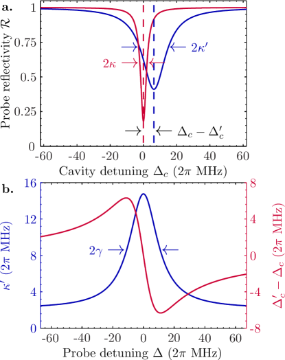
Figure 2: (Color online) (a) Calculated probe reflectivity spectrum as a function of cavity detuning $\Delta_{\mathrm{c}}$ for an empty cavity (red line) and for $N=500$ ions interacting with the cavity field (blue line) [see Eq. (13)] for a probe detuning of $\Delta=\gamma$. The coupling of the ions and the cavity mode lead to a broadening and a shift of the resonance dip. The values of the parameters are set to typical values used in the experiments presented in Secs. III and IV: $\kappa=2\pi\times 2.1~{}\mathrm{MHz}$, $\kappa_{1}=2\pi\times 1.5~{}\mathrm{MHz}$, $\gamma=2\pi\times 11.2~{}\mathrm{MHz}$, $g=2\pi\times 0.53~{}\mathrm{MHz}$. (b) Expected effective cavity decay rate $\kappa^{\prime}$ and shift of the cavity resonance $\Delta^{\prime}_{\mathrm{c}}-\Delta_{\mathrm{c}}$ as a function of probe detuning $\Delta$ calculated for the same set of parameters.

In steady-state, the mean value of the intracavity field amplitude is given by

$$a=\frac{\sqrt{2\kappa_{1}/\tau}a_{\mathrm{in}}}{\kappa^{\prime}+i\Delta_{\mathrm{c}}^{\prime}},$$ (5)

where an effective cavity decay rate and an effective cavity detuning are introduced:

$$\kappa^{\prime} = \kappa+g^{2}N\frac{\gamma}{\gamma^{2}+\Delta^{2}},$$ (6)

$$\Delta_{\mathrm{c}}^{\prime} = \Delta_{\mathrm{c}}-g^{2}N\frac{\Delta}{\gamma^{2}+\Delta^{2}}.$$ (7)

In these expressions, $N$ is the effective number of ions interacting with the intracavity field, which is calculated by summing over all ions and weighting the contribution of each ion by the field modefunction under consideration evaluated at the ion’s position:

$$N=\sum_{j=1}^{N_{\mathrm{tot}}}\Psi_{\mathrm{00}}^{2}(\bm{r}_{j}).$$ (8)

Here,

$$\Psi_{00}^{2}(\bm{r})= \left(\frac{w_{0}}{w(z)}\right)^{2}\exp\left(-\frac{2r^{2}}{w(z)^{2}}\right)$$

$$\times\sin^{2}\left[kz-\arctan(z/z_{0})+kr^{2}/2R(z)\right],$$ (9)

is the modefunction of the cavity fundamental TEM₀₀ Gaussian mode with waist $w_{0}$ at the center of the mode and $w(z)=w_{0}\sqrt{1+z^{2}/z_{0}^{2}}$, $R(z)=z+z_{0}^{2}/z$, $z_{0}=\pi w_{0}^{2}/\lambda$, and $k=2\pi/\lambda$.

Large ion Coulomb crystals in a linear radiofrequency trap are to an excellent approximation spheroids with half-length $L$ and radius $R$ (see Fig. 5), where the density of ions, $\rho$, is constant throughout the crystal Drewsen1998 ; Hornekaer2002Formation . It is then convenient to adopt a continuous medium description, in which Eq. (8) becomes an integral over the crystal volume $V$:

$$N=\rho\int_{V}d\bm{r}\Psi_{00}^{2}(\bm{r})$$ (10)

In our experiment, the crystal radius and half-length, $R$ and $L$, are typically much smaller than $z_{0}$ and the axial mode function can be approximated by $\sin^{2}(kz)$. Moreover, for randomly distributed ions along the cavity axis $z$, one can average over the cavity standing-wave longitudinal structure, which gives an effective number of ions equal to

$$N=\frac{\rho}{2}\int_{V}d\bm{r}\exp[-2r^{2}/w(z)^{2}].$$ (11)

This expression can be evaluated knowing the crystal dimensions, its density, and the cavity mode geometry. For typical crystals with large radial extension as compared to the cavity waist $R\gg w_{0}$ and length smaller than the Rayleigh range $L\ll z_{0}$, this expression reduces to

$$N\simeq\rho\frac{\pi w_{0}^{2}}{4}L,$$ (12)

which is simply the product of the ion density by the volume of the cavity mode in the crystal.

Using the input-output relation $a_{\mathrm{r}}=\sqrt{2\kappa_{1}\tau}a-a_{\mathrm{in}}$, one finds that the steady-state probe reflectivity spectrum of the cavity is also Lorentzian-shaped in presence of the ions, the bare cavity decay rate, and detuning $\kappa$ and $\Delta_{\mathrm{c}}$ being replaced by their effective counterparts $\kappa^{\prime}$ and $\Delta_{\mathrm{c}}^{\prime}$ of Eqs. (6,7):

$$\mathcal{R}\equiv\left|\frac{a_{r}}{a_{\mathrm{in}}}\right|^{2}=\left|\frac{2\kappa_{1}-\kappa^{\prime}-i\Delta_{\mathrm{c}}^{\prime}}{\kappa^{\prime}+i\Delta_{\mathrm{c}}^{\prime}}\right|^{2}.$$ (13)

The broadening and shift of the cavity resonance then represent the change in absorption and dispersion experienced by the cavity field interacting with $N$ ions. In Fig. 2 (a) the expected cavity reflectivity spectrum is shown for both an empty cavity and a cavity containing a crystal with an effective number of ions $N=500$ and for parameters corresponding to those used in the experiments presented in Secs. III and IV. In Fig. 2 (b) the effective cavity decay rate, $\kappa^{\prime}$, and the shift of the cavity resonance induced by the interaction with the ions, $\Delta^{\prime}_{\mathrm{c}}-\Delta_{\mathrm{c}}$, are shown as a function of the probe detuning, $\Delta$, for the same parameters.

II.3 Effect of the motion of the ions

The interaction Hamiltonian in Eq. (2) is only valid for atoms at rest. If an ion is moving along the axis of the cavity, the standing-wave structure of the cavity field and the Doppler shifts due to the finite velocity of the ion have to be taken into account. For an ion moving along the standing wave field with a velocity $v_{j}$, it is convenient to define atomic dipole operators, $\sigma_{j\pm}=\frac{1}{2}\sigma_{j}\exp{(\pm ikz_{j})}$, arising from the interaction with the two counterpropagating components of the standing-wave cavity field. In the low saturation limit and taking into account the opposite Doppler-shifts, the evolution equations (3),(4) become

$$\dot{\sigma}_{j\pm} = -\left[\gamma+i(\Delta\pm kv_{j})\right]\sigma_{j\pm}+i(g/2)\Psi_{\mathrm{nm}}(\bm{r}_{j})a$$ (14)

$$\dot{a} = -(\kappa+i\Delta_{\mathrm{c}})a+i(g/2)\sum_{j=1}^{N_{tot}}\Psi_{\mathrm{nm}}(\bm{r}_{j})\left(\sigma_{j+}+\sigma_{j-}\right)+\sqrt{2\kappa_{1}/\tau}a_{\mathrm{in}}.$$ (15)

When the typical timescale of the motion is slow as compared to the timescales for the coupled dynamics of the atomic dipole and cavity field, the steady-state mean value of the intracavity field can be found by averaging the contributions of the individual dipole mean values given by Eq. (14) over the distribution of the mean velocities, $f(v)$. For a distribution $f(v)$ with an average velocity $v_{\mathrm{D}}$ a conservative estimate for this to be valid is that the mean Doppler-shift is smaller than both effective rates of the coupled system on resonance ($\Delta_{\mathrm{c}}=\Delta=0$), $kv_{\mathrm{D}}\ll\min[\kappa+g^{2}N/\gamma,\gamma+g^{2}N/\kappa]$. Under these conditions, the expression for the intracavity field mean value is then of the same form as in the zero-velocity case (Eq. (5)). The effective cavity field decay rate and detuning of Eqs. (6) and(7) are modified according to

$$\kappa^{\prime} = \kappa+g^{2}N\int{\mathrm{d}}vf(v)\gamma\xi(v)$$ (16)

$$\Delta_{\mathrm{c}}^{\prime} = \Delta_{\mathrm{c}}-g^{2}N\int{\mathrm{d}}vf(v)(\Delta-kv)\xi(v).$$ (17)

where

$$\xi(v)=\frac{\gamma^{2}+\Delta^{2}+(kv)^{2}}{(\gamma^{2}+\Delta^{2})^{2}+2(\gamma^{2}-\Delta^{2})(kv)^{2}+(kv)^{4}}.$$ (18)

In the case of a thermal Maxwell-Boltzmann distribution with temperature $T$, one has $f(v)=\sqrt{\frac{m}{2\pi k_{\mathrm{B}}T}}\exp\left(-\frac{mv^{2}}{2k_{\mathrm{B}}T}\right)$, where $k_{\mathrm{B}}$ is the Boltzmann constant and $m$ the mass of the ion. At low temperatures, i.e., when the width of the thermal distribution is small as compared to the atomic natural linewidth, the effective cavity field decay rate and detuning given by Eqs. (16) and (17) are well-approximated by

$$\kappa^{\prime} = \kappa+g^{2}N\frac{\gamma^{\prime}}{{\gamma^{\prime}}^{2}+\Delta^{2}},$$ (19)

$$\Delta_{\mathrm{c}}^{\prime} = \Delta_{\mathrm{c}}-g^{2}N\frac{\Delta}{{\gamma^{\prime}}^{2}+\Delta^{2}}.$$ (20)

These equations are of the same form as Eqs. (6) and (7), replacing the natural dipole decay rate by an effective dipole decay rate ,

$$\gamma^{\prime}\simeq\gamma(1+kv_{\mathrm{D}}/\sqrt{2}),$$ (21)

where $v_{\mathrm{D}}=\sqrt{k_{B}T/m}$ is the mean Doppler velocity.

III Experimental setup

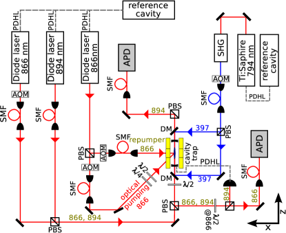
Figure 3: (Color online) Schematic experimental setup. The abbreviations are: polarizing beam splitter (PBS), single mode fiber (SMF), acousto-optical modulator (AOM), dichroic mirror (DM), Pound-Drever-Hall lock (PDHL), avalanche photodiode (APD), second harmonic generation (SHG). The photoionization laser is not shown.

III.1 Cavity trap

The ion trap used is a segmented linear quadrupole radiofrequency trap that consists of four cylindrical electrode rods (for details see Herskind2008Loading ). The electrode radius is $2.60~{}\mathrm{mm}$ and the distance from the trap center to the electrodes is $r_{0}=2.35~{}\mathrm{mm}$. Each electrode rod is divided into three parts, where the length of the center electrode is $z_{\mathrm{C}}=5.0~{}\mathrm{mm}$, and the length of the end electrodes is $z_{\mathrm{E}}=5.9~{}\mathrm{mm}$. Radial confinement is achieved by a radiofrequency field (RF) applied to the entire rods at a frequency of $2\pi\times 4~{}\mathrm{MHz}$ and a $\pi$ phase difference between neighboring rods. The axial trapping potential is created by static voltages (DC) applied to the outer parts of the rods.

An optical cavity is incorporated into the trap with its axis parallel to the symmetry axis of the ion trap (see Fig. 3). The cavity mirrors have a diameter of $1.2~{}\mathrm{mm}$ and a radius of curvature of $10~{}\mathrm{mm}$. The rear face of both mirrors are anti-reflection coated at a wavelength of $866~{}\mathrm{nm}$ corresponding to the $3\mathrm{d}^{2}\mathrm{D}_{3/2}\leftrightarrow 4\mathrm{p}^{2}\mathrm{P}_{1/2}$ transition in ${}^{40}\mathrm{Ca}^{+}$, while the front facade of one mirror is partially transmitting (PT) and for the other highly reflecting (HR) at this wavelength. Their intensity transmission coefficients are $1500$ and $5~{}\mathrm{ppm}$, respectively. The intracavity losses due to contamination of the mirrors during the initial bake out amount to $\sim 650$ ppm. The PT mirror is mounted on a plate that can be translated using piezoelectric actuators to allow for scanning or actively stabilizing the cavity length. The cavity has a close to confocal geometry with a length of $11.8~{}\mathrm{mm}$, corresponding to a free spectral range of $12.7~{}\mathrm{GHz}$ and a waist of the fundamental $\mathrm{TEM_{00}}$ mode of $w_{0}=37\mathrm{\mu m}$. With a measured cavity field decay rate of $\kappa=2\pi\times(2.1\pm 0.1)~{}\mathrm{MHz}$, the finesse is found to be $\mathcal{F}=3000\pm 200$ at a wavelength of $866~{}\mathrm{nm}$ Herskind2008Loading .

${}^{40}\mathrm{Ca}^{+}$ ions are loaded into the trap by in situ photoionization of atoms from a beam of atomic calcium in a two-photon resonant photoionization process Kjaergaard2000Isotope ; Mortensen2004Isotope ; Herskind2008Loading . The ions are cooled to a crystalline state through Doppler-laser cooling using a combination of two counterpropagating laser beams, resonant with the $4\mathrm{s}^{2}\mathrm{S}_{1/2}\leftrightarrow 4\mathrm{p}^{2}\mathrm{P}_{1/2}$ transition at 397 nm along the trap axis, and a repumping laser applied along the $x$ axis and resonant with the $3\mathrm{d}^{2}\mathrm{D}_{3/2}\leftrightarrow 4\mathrm{p}^{2}\mathrm{P}_{1/2}$ transition at 866 nm to prevent shelving to the metastable $\mathrm{D}_{3/2}$ state. Three sets of Helmholtz coils are used to compensate for residual magnetic fields and to produce bias magnetic fields. For the measurements of the collective coupling rate between the ion Coulomb crystals and the cavity light field, the transverse magnetic fields along $x$ and $y$ are nulled and a magnetic field of $B_{\mathrm{z}}\sim 2.5~{}{G}$ along the $z$-axis is used.

III.2 Detection

A grating stabilized diode laser at $866~{}\mathrm{nm}$ provides the light for probing the coupling of the ion Coulomb crystals with the standing wave field inside the optical cavity. It is injected into the cavity through the PT mirror. Additionally, a second grating stabilized diode laser with a wavelength of $894~{}\mathrm{nm}$ serves as an off-resonant reference laser and is simultaneously coupled to the cavity through the PT mirror and used to monitor the cavity resonance. Both lasers are frequency stabilized to the same temperature stabilized reference cavity and have linewidths of $\sim 100~{}\mathrm{kHz}$.

The reflectivity of the 866-nm cavity field is measured using an avalanche photo diode (APD). The light sent to the APD is spectrally filtered by a diffraction grating ($1800~{}\mathrm{lines/mm}$) and coupled to a single mode fiber. Taking into account the efficiency of the APD at $866~{}\mathrm{nm}$, the fiber incoupling and the optical losses, the total detection efficiency amounts to $\approx 16\%$. A similar detection system is used to measure the transmission of the 894-nm reference laser.

Depending on the experiment, the reference laser serves two different purposes. In a first configuration, the length of the cavity is scanned at a rate of $30~{}\mathrm{Hz}$ over the atomic resonance. In this configuration, the frequency of the reference laser is tuned such that it is resonant at the same time as the probe laser in the cavity scan. This allows for monitoring slow drifts and acoustic vibrations. The signal of the weak probe laser is then averaged over typically 100 scans in which the stronger reference laser is used to keep track of the current position of the cavity resonance.

In a second configuration, the cavity resonance is locked on the atomic resonance by stabilizing the length of the cavity to the frequency of the reference laser in a Pound-Drever-Hall locking scheme Drever1983Laser . During the measurement, imperfections in the stabilization are compensated for by monitoring the transmission of the 894-nm reference laser. The data is then postselected by only keeping data points for which the transmitted reference signal was above a certain threshold.

III.3 Experimental sequence

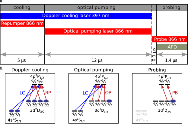
Figure 4: (color online) (a) Experimental sequence used to measure the collective coupling rate. (b) Energy levels of ${}^{40}\mathrm{Ca}^{+}$ including the relevant transitions addressed in the three parts of the experimental sequence. The acronyms are: laser cooling beam (LC), repumping beam (RP), optical pumping beam (OP), probe beam (PB), avalanche photodiode (APD).

In both configurations, the cavity reflection spectrum is measured at a rate of $50~{}\mathrm{kHz}$ using a $20~{}\mathrm{\mu s}$ sequence of Doppler cooling, optical pumping and probing, as indicated in Fig. 4. First, the ions are Doppler-laser cooled for $5~{}\mathrm{\mu s}$ by driving the $4\mathrm{s}^{2}\mathrm{S}_{1/2}\leftrightarrow 4\mathrm{p}^{2}\mathrm{P}_{1/2}$ transition using laser cooling beams at 397 nm (LC), and at the same time repumping on the $3\mathrm{d}^{2}\mathrm{D}_{3/2}\leftrightarrow 4\mathrm{p}^{2}\mathrm{P}_{1/2}$ transition with a laser at 866 nm (RP). Next, the ions are optically pumped to the ${m_{\mathrm{J}}}=+3/2$ magnetic substate of the $3\mathrm{d}^{2}\mathrm{D}_{3/2}$ level by applying the optical pumping laser (OP) in combination with the laser cooling beams (LC) for a period of $12~{}\mathrm{\mu s}$. The optical pumping laser is resonant with the $3\mathrm{d}^{2}\mathrm{D}_{3/2}\leftrightarrow 4\mathrm{p}^{2}\mathrm{P}_{1/2}$ transition and has a polarization consisting only of $\sigma^{+}$- and $\pi$-polarized components. It is sent to the trap under an angle of $45^{\circ}$ with respect to the quantization axis. By probing the populations of the different Zeeman sublevels, the efficiency of the optical pumping was measured to be $\eta=97^{+3}_{-5}\%$ phdPeterHerskind . Finally, the cavity reflection signal is probed by injecting a $1.4~{}\mathrm{\mu s}$ $\sigma^{-}$-polarized probe pulse, resonant with the $3\mathrm{d}^{2}\mathrm{D}_{3/2}\leftrightarrow 4\mathrm{p}^{2}\mathrm{P}_{1/2}$ transition, into the $\mathrm{TEM}_{00}$ mode of the optical cavity. Its intensity is set such that the mean intracavity photon number is less than one at any time. With a delay of $0.1~{}\mathrm{\mu s}$ relative to the probe laser, the APD is turned on. The delay ensures that the field has built up inside the cavity and that the system has reached a quasi-steady-state. The length of the probing period was chosen in order to minimize the total sequence length as well as to avoid depopulation due to saturation of the transition phdPeterHerskind .

III.4 Effective number of ions

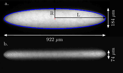
Figure 5: (Color online) (a) Typical projection image of a crystal used in collective strong coupling measurements. All ions are exposed to cooling and repumping light. The solid blue line indicates the outline of the ellipsoid. (b) Same crystal, but only the ions in the cavity mode are exposed to repumping light, now injected into the cavity. The ions outside the cavity mode volume are not visible, as they are shelved into the metastable $3\mathrm{d}^{2}\mathrm{D}_{3/2}$ level. The crystal contains $N_{\mathrm{tot}}=8780\pm 180$ ions, of which $N=489^{+18}_{-27}$ effectively interact with the cavity field.

As mentioned above, the effective number of ions interacting with the cavity field depends on the ion crystal density and the overlap between the crystal and the cavity modevolume, where the density of the ion Coulomb crystals depends on the amplitude of the RF voltage Hornekaer2001 :

$$\rho=\frac{\epsilon_{0}U_{\mathrm{RF}}^{2}}{Mr_{0}^{4}\Omega_{\mathrm{RF}}^{2}}.$$ (22)

Here, $M$ denotes the ion mass. The precise calibration of the RF voltage on the trap electrodes can be performed, e.g., on the basis of a zero-temperature charged liquid model Turner1987Collective ; Hornekaer2001 ; Herskind2009Positioning or the measurement of the Wigner-Seitz radius Herskind2009Positioning . For the trap used in these experiments, $\rho=(6.01\pm 0.08)\times 10^{3}~{}U_{\mathrm{RF}}^{2}~{}\mathrm{V^{-2}cm^{-3}}$. The crystal mode volume is found by taking fluorescence images of the crystal during Doppler-laser cooling, as shown in Fig. 5, from which the crystal half-length $L$ and radius $R$ can be extracted. Taking a possible offset between the cavity axis and the crystal revolution axis into account, the effective number of ions [see Eq. (11)] is then numerically calculated using the formula

$$N=\eta\frac{\rho}{2}\int_{V}\mathrm{d}x\mathrm{d}y\;\exp\left\{-2[(x-x_{0})^{2}+(y-y_{0})^{2}]/w_{0}^{2}\right\},$$ (23)

where the parameter $\eta$ accounts for a finite efficiency of the optical pumping preparation and $x_{0}$ and $y_{0}$ denote the radial offsets. These offsets can in principle be canceled to within a micron Herskind2009Positioning , but in the experiments reported here, they were measured to be $x_{0}=3.9~{}\mathrm{\mu m},~{}y_{0}=15.7~{}\mathrm{\mu m}$ Dantan2009Large . The uncertainty in the effective number of ions comes from the uncertainty $\delta\rho$ in the density determination, due to the RF voltage calibration, the uncertainty in the crystal volume $\delta V$, due to the imaging resolution $\delta x$ and the uncertainty of the optical pumping efficiency $\delta\eta$. The relative uncertainty in the effective number of ions, $N=\eta\rho V$, can then be expressed as phdPeterHerskind

$$\frac{\delta N}{N}=\sqrt{\left(\frac{\delta\rho}{\rho}\right)^{2}+\left(\frac{\delta V}{V}\right)^{2}+\left(\frac{\delta\eta}{\eta}\right)^{2}},$$ (24)

where $\delta V/V=\delta x\sqrt{16L^{2}+R^{2}}/2RL$. For the typically few-mm-long prolate crystals used in these experiments and an imaging resolution $\delta x\sim$ $\mu$m, this results in a relative uncertainty of 5-7% in the effective number of ions.

IV Collective coupling measurements

To achieve collective strong coupling on the chosen $3\mathrm{d}^{2}\mathrm{D}_{3/2},\;m_{\mathrm{J}}=+3/2\leftrightarrow 4\mathrm{p}^{2}\mathrm{P}_{1/2},\;m_{\mathrm{J}}=+1/2$ transition the collective coupling rate $g\sqrt{N}$ has to be larger than the cavity field decay rate $\kappa=2\pi\times 2.1$ MHz and the optical dipole decay rate $\gamma=2\pi\times 11.2$ MHz. With the known dipole element of the transition and the cavity geometry, the single-ion coupling rate at an antinode at the center of the cavity fundamental mode is expected to be $g=2\pi\times(0.53\pm 0.01)$ MHz. One thus expects to be able to operate in the collective strong coupling regime as soon as $N\gtrsim 500$.

IV.1 Atomic absorption and dispersion

To investigate the coherent coupling of the ions with the cavity field in the collective strong coupling regime, we first perform measurements of the atomic absorption and dispersion of a given crystal with $N\sim 500$ by scanning the cavity length around atomic resonance and recording the probe reflectivity spectrum. The crystal used in these experiments is similar to the one shown in Fig. 5. With a density of $\rho=(5.4\pm 0.1)\times 10^{8}~{}\mathrm{cm}^{-3}$ , a half-length $L=(511\pm 1)~{}\mathrm{\mu m}$ and radius $R=(75\pm 1)~{}\mathrm{\mu m}$ the total number of ions in the crystal is $N_{\mathrm{tot}}=6500\pm 200$, and the effective number of ions interacting with the cavity mode is $N=520^{+24}_{-32}$.

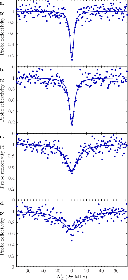
Figure 6: (Color online) Typical probe reflectivity for various values of the atomic detuning $\Delta$. The probe detunings were (a) $\Delta\approx 2\pi\times 54.3~{}\mathrm{MHz}$, (b) $\Delta\approx 2\pi\times 24.3~{}\mathrm{MHz}$, (c.) $\Delta\approx 2\pi\times 8.3~{}\mathrm{MHz}$, and (d.) $\Delta\approx 2\pi\times 0.3~{}\mathrm{MHz}$. Solid lines are Lorentzian fits to the data; the effective cavity field decay rate $\kappa^{\prime}$ is deduced from the fit.

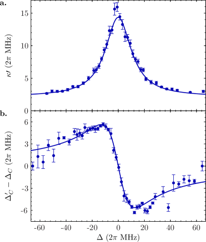
Figure 7: (Color online) (a) Measured cavity field effective decay rate $\kappa^{\prime}$ versus probe detuning $\Delta$ for a crystal with $N=520^{+24}_{-32}$ ions interacting with the cavity field. The blue solid line is a fit to the data. (b) Measured shift of the cavity resonance frequency $\Delta_{\mathrm{c}}^{\prime}-\Delta_{\mathrm{c}}$ versus atomic detuning $\Delta$ for the same crystal. The blue line is a fit to the data.

The broadening and the shift of the cavity resonance are then measured as a function of the detuning of the probe laser, $\Delta$. This is accomplished by scanning the cavity length over a range corresponding to $\sim 1.3~{}\mathrm{GHz}$ at a repetition rate of $30~{}\mathrm{Hz}$, for a fixed value of $\Delta$. The width of the reflection dip for a given detuning $\Delta$ is found by averaging over 100 cavity scans, where the reference laser is overlapped with the probe laser on the cavity scan and used to compensate for any drift of the cavity. In Fig. 6, cavity reflection scans are plotted for various detunings. Each data point corresponds to the average of 100 $20-\mathrm{\mu s}$-measurement sequences as showed in Fig. 4. As expected from Eq. (19), the broadening of the intracavity field absorption reflects the two-level atomic medium absorption. Each set of data is, according to Eq. (13), fitted to a Lorentzian from which the cavity half width half maximum (HWHM) $\kappa^{\prime}$ is deduced. Figure 7(a) shows the modified cavity HWHM, $\kappa^{\prime}$, as a function of detuning of the probe laser, $\Delta$. Each point is the average of five measurements; the solid line is a fit according to Eq. (19). From the fit we deduce a collective coupling rate of $g_{\mathrm{N}}=2\pi\times(12.2\pm 0.2)~{}\mathrm{MHz}$, in good agreement with the theoretical expectation of $g_{\mathrm{N,~{}theory}}=2\pi\times(12.1^{+0.4}_{-0.5})~{}\mathrm{MHz}$, calculated for $N=520^{+24}_{-32}$ ions interacting with the cavity mode Herskind2009Realization . Furthermore, the effective dipole decay rate $\gamma^{\prime}$ is left as a fit parameter to account for nonzero temperature effects, as discussed in Sec. II.3. The fit yields $\gamma^{\prime}=2\pi\times(11.9\pm 0.4)~{}\mathrm{MHz}$, which would correspond to a temperature of $T=24^{+20}_{-14}~{}\mathrm{mK}$, and a natural half-width of the cavity of $\kappa=2\pi\times(2.2\pm 0.1)~{}\mathrm{MHz}$, in good agreement with the value deduced from an independent measurement of the free spectral range (FSR) and the finesse of the cavity, $\kappa=2\pi\times(2.1\pm 0.1)~{}\mathrm{MHz}$ Herskind2008Loading .

For the measurement of the effective cavity detuning, $\Delta_{\mathrm{c}}^{\prime}$, the position of the 894-nm resonance laser in the cavity scan is fixed to the bare cavity resonance. The frequency shift is then measured by comparing the position of the probe and the reference signal resonances in the cavity scan. The effective cavity detuning as a function of probe detuning is shown in Fig. 7(b) One observes the typical dispersive frequency-shift of two-level atoms probed in the low saturation regime. The data is fitted to the theoretical model according to Eq. (20), to find a collective coupling rate $g_{\mathrm{N}}=2\pi\times(12.0\pm 0.3)~{}\mathrm{MHz}$ and an effective dipole decay rate $\gamma^{\prime}=2\pi\times(12.7\pm 0.8)~{}\mathrm{MHz}$. Both values are consistent with the previous measurement and the theoretical expectations. As in the previous measurement, the 894-nm reference laser is used to compensate systematic drifts and acoustic vibrations. However, since this compensation method relies on the temporal correlations of the drifts in both signals, and thereby on their relative positions in the cavity scan, the compensation becomes less effective at large detunings. This is reflected in the bigger spread and the larger error bars at larger detunings, which renders this method slightly less precise than the absorption measurement to evaluate the collective coupling rate.

IV.2 Vacuum Rabi splitting

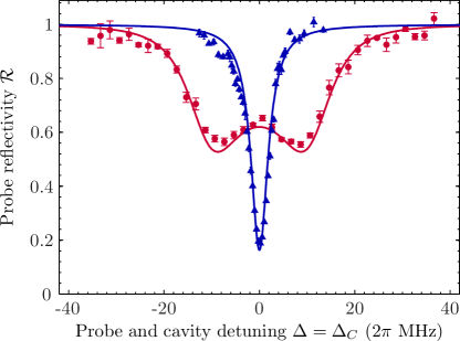
Figure 8: (color online). Probe reflectivity signal as a function of $\Delta=\Delta_{\mathrm{c}}$ for the empty cavity (blue triangles) and with a crystal with $N=520^{+24}_{-32}$ effectively interacting ions present in the cavity mode volume (red circles). The solid lines are fits to the theory.

A third complementary method to measure the collective coupling rate is based on locking the cavity on atomic resonance, $\omega_{\mathrm{c}}=\omega_{\mathrm{at}}$. The response of the coupled atom-cavity system is then probed as a function of probe detuning $\Delta$, which is then equal to the cavity detuning $\Delta_{\mathrm{c}}$. The result of this measurement is shown on Fig. 8. The blue triangles are obtained with an empty cavity, while the red circles were taken with the same ion Coulomb crystal as used in the previous experiments. Each data point is deduced from $2\times 10^{4}$ experimental sequences (see Fig. 4). The results are fitted using the theoretical expectations of Eq. (13) and Eqs. (19) and (20) (solid lines in Fig. 8) and yield $g_{\mathrm{N}}=2\pi\times(12.2\pm 0.2)~{}\mathrm{MHz}$, a value that is in good agreement with the previous measurements. To facilitate the convergence of the more complex fitting function, the value of $\gamma^{\prime}$ in Eqs. (19) and (20) was set to the one found in the previous absorption measurement.

From these three independent measurements of the collective coupling rate $g_{\mathrm{N}}$ and using the effective number of ions $N=520^{+24}_{-32}$, one deduces a single ion coupling rate of $g_{\mathrm{exp}}=2\pi\times(0.53\pm 0.02)~{}\mathrm{MHz}$, which is in excellent agreement with the expected value of $g_{\mathrm{theory}}=2\pi\times(0.53\pm 0.01)~{}\mathrm{MHz}$.

IV.3 Scaling with the number of interacting ions

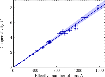
Figure 9: (Color online) Cooperativity as a function of the effective number of ions. The solid line is a linear fit to the data and yields a scaling parameter of $\frac{C}{N}=(5.1^{+0.4}_{-0.2})\times 10^{-3}$. The shaded area indicates the confidence region for the upper and lower limit of $C$ determined by the (systematic) uncertainties on the effective number of ions, $N$. The dashed line indicates the strong collective coupling limit $g_{\mathrm{N}}>(\kappa,\gamma)$.

To check further the agreement between the theoretical predictions and the experimental data, we investigated the dependence of the collective coupling rate on the effective number of ions. An attractive feature of ion Coulomb crystals is that the number of ions effectively interacting with a single mode of the optical cavity can be precisely controlled by the trapping potentials. While the density $\rho$ only depends on the amplitude of the RF voltage [see Eq. (22)], the aspect ratio of the crystal depends on the relative trap depths of the axial and radial confinement potentials, which can be independently controlled by the DC voltages on the endcap electrodes. This allows for controlling the number of effectively interacting ions down to the few ion-level.

By analogy with the case of a single two-level system interacting with a single field mode of an optical cavity, the cooperativity parameter $C$ is defined here as (half) the ratio of the square of the effective coupling rate $g_{\mathrm{N}}$ to the cavity field decay rate $\kappa$ times the effective dipole decay rate $\gamma^{\prime}$ (taking into account the effect of the motion of the ions): $C=g_{\mathrm{N}}^{2}/2\kappa\gamma^{\prime}$. As can be seen from Eq. (19), this parameter can be experimentally obtained by measuring for a probe field tuned to atomic resonance ($\Delta=0$) the effective cavity field decay rate $\kappa^{\prime}(\Delta=0)=\kappa+\frac{g_{\mathrm{N}}^{2}}{\gamma^{\prime}}=\kappa~{}(1+2C)$. In Fig. 9, the dependence of the cooperativity parameter, $C$, is plotted as a function of the effective number of ions interacting with the TEM₀₀ mode, where the effective number of ions was changed by measuring for different aspect ratios and densities of several crystals.

The effective number of ions in each crystals was deduced by applying the method described in Sec. III.4. The data points were obtained using $\sigma^{-}$-circularly polarized probe light, hence probing the population in the $m_{\mathrm{J}}=+3/2$ and $m_{\mathrm{J}}=+1/2$ substates, and shows the expected linear dependence on the effective number of ions. From a linear fit (solid line) we deduce a scaling parameter $\frac{C}{N}=(5.1^{+0.4}_{-0.2})\times 10^{-3}$. The limit where collective strong coupling is achieved ($g_{\mathrm{N}}>\kappa,\gamma$) is indicated by the black dashed line and is reached for $\approx 500$ interacting ions.
The largest coupling observed in these experiments was measured for a crystal with a length of $\sim 3~{}\mathrm{mm}$ and a density of $\sim 6\times 10^{8}~{}\mathrm{cm^{-3}}$ and amounted to $C=7.9\pm 0.3$, corresponding to an effective number of ions of $N=1523^{+69}_{-93}$. This value exceeds previously measured cooperativities with ions in optical cavities by roughly one order of magnitude Guthohrlein2001AsingleIon ; Keller2004Continuous ; Kreuter2004 .

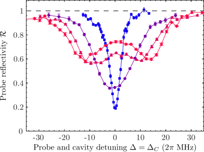
Figure 10: (color online). Vacuum Rabi splitting spectra ($\Delta=\Delta_{\mathrm{c}}$) obtained for increasing effective number of ions [0 (blue squares), 243 (lilac circles), 601 (dark red triangles), 914 (red diamonds)], the lines are presented to guide the eye.

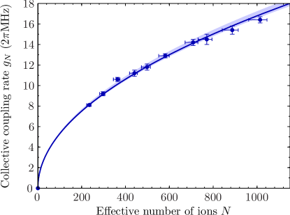
Figure 11: (color online). Collective coupling rate $g_{\mathrm{N}}$ versus effective number of ions $N$ deduced from reflectivity spectra, such as shown in Fig. 10, obtained with crystals of different shape and density. The blue line is a fit to the data and gives a single ion coupling rate $g=2\pi\times(0.53\pm 0.01)$ MHz. The shaded area indicates the lower and upper bound of the collective coupling rate $g_{\mathrm{N}}$ within the uncertainties of $N$. The horizontal errorbars are calculated according to Eq. (24)

Similarly, vacuum Rabi splitting spectra, such as the one presented in Fig. 8, were measured for several crystals and aspect ratios. The result of such measurements is shown in Fig. 10, showing clearly the increase in the separation between the coupled crystal+cavity normal modes as the number of ions is increased. The collective coupling rate $g_{\mathrm{N}}$, derived from fits to the theoretical expression Eq. (13), is plotted for different effective number of ions in Fig. 11. Taking the finite optical pumping efficiency into account and fitting the curve with the expected square-root dependency, we deduce a single ion coupling rate of $g=2\pi\times(0.53\pm 0.01)~{}\mathrm{MHz}$, in good agreement with the previous measurements and the theoretical expectation.

V Coherence time of collective Zeeman substate coherences

To evaluate the prospect for realizing coherent manipulations, we measured the decay time of the collective coherences between the Zeeman substates of the $3\mathrm{d}^{2}\mathrm{D}_{3/2}$ level. These coherences were established by the Larmor precession of the magnetic spin induced by an additional $B$-field transverse to the quantization axis. In presence of this orthogonal $B$-field, the population of the several substates undergo coherent oscillations, which are measured at different times in their free evolution by directly probing the coherent coupling between the cavity field and the ions. In order to be able to resolve the coherent population oscillations in time using the previous technique (probing time $\sim 1~{}\mathrm{\mu s})$ the amplitude of the longitudinal $B$-field was lowered to obtain oscillation periods in the $\sim 10~{}\mathrm{\mu s}$ range, and the optical pumping preparation was modified as to minimize the effect of the transverse $B$-field. The reduced $B$-field along the quantization axis could in principle make the sample more sensitive to $B$-field fluctuations. Since these fluctuations might be one of the factors eventually limiting the achievable coherence time, we expect the coherence time measured by this method to be a lower bound as compared to the previous configuration with a larger longitudinal $B$-field.

V.1 Experimental sequence and theoretical expectations

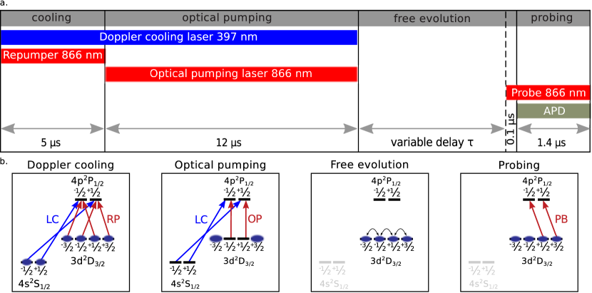
Figure 12: (Color online) (a) Experimental sequence used to measure the coherence time of collective Zeeman substate coherences in the $3\mathrm{d}^{2}\mathrm{D}_{3/2}$ level. (b) Energy levels of ${}^{40}\mathrm{Ca}^{+}$, including the relevant transitions and their polarization for the four phases of the experimental cycle. In the third phase, all lasers are turned off for a variable delay $\tau$, and the system evolves freely in presence of a transverse magnetic field component $B_{\mathrm{x}}$.

The coherence time measurements required the experimental configuration and the measurement sequence to be slightly modified as compared to the collective coupling rate measurements described in Sec. III.3. The Larmor precession is induced by an additional $B$-field component along the transverse $x$ direction, while the longitudinal magnetic field component $B_{\mathrm{z}}$ was lowered to optimize the contrast of the coherent population oscillations. The optical pumping light propagates along the $x$ axis and is $\pi$-polarized, hence transferring most of the atoms symmetrically into the two outermost magnetic sub-states of the $3\mathrm{d}^{2}\mathrm{D}_{3/2}$ level, $m_{\mathrm{J}}=\pm 3/2$.

The experimental sequence used to measure the coherence time is shown in Fig. 12. The ions are Doppler-laser cooled during the first $5~{}\mathrm{\mu s}$, followed by a $12~{}\mathrm{\mu s}$ optical pumping period. After the optical pumping, all lasers are turned off for a time $\tau$, allowing for the free evolution of the system. Finally, a weak $\sigma^{-}$-circularly polarized probe pulse is injected into the cavity, addressing the ions in the $m_{\mathrm{J}}=+1/2$ and $m_{\mathrm{J}}=+3/2$ sub-states. The steady-state cavity reflection is measured by collecting the reflected photons with the APD for $0.5~{}\mathrm{\mu s}$. The additional delay time between optical pumping preparation and probing obviously lowers the repetition rate of the sequence significantly, especially for long delay times, and the number of data points for each sweep of the cavity will decrease. To compensate for this, the data points at longer delays had to be averaged over more cavity scans, which substantially increased the acquisition time and eventually limited these measurements to delays of around $\sim 120~{}\mathrm{\mu s}$.

Based on a simple four-level model the free Larmor precession-induced changes in the populations of the Zeeman substates, $\left|m_{\mathrm{J}}=\pm\nicefrac{{1}}{{2}},~{}\pm\nicefrac{{3}}{{2}}\right\rangle$, of the $3\mathrm{d}^{2}\mathrm{D}_{3/2}$ level can be calculated. For a homogeneous $B$-field with components $B_{\mathrm{x}}$ and $B_{\mathrm{z}}$, the Hamiltonian of the four-level system can be expressed in terms of collective population operator,

$$\hat{\Pi}_{{m_{\mathrm{J}}}}=\sum_{j=1}^{N_{\mathrm{t}ot}}\left|m_{\mathrm{J}}\right\rangle^{(j)}\left\langle m_{\mathrm{J}}\right|^{(j)},$$ (25)

and collective spin operators

$$\hat{\sigma}_{{m_{\mathrm{J}},m_{\mathrm{J}}^{\prime}}}=\sum_{j=1}^{N_{\mathrm{t}ot}}\left|m_{\mathrm{J}}\right\rangle^{(j)}\left\langle m_{\mathrm{J}}^{\prime}\right|^{(j)},\quad m_{\mathrm{J}}\neq m_{\mathrm{J}}^{\prime}.$$ (26)

Here, $\left|m_{\mathrm{J}}\right\rangle^{(j)}$ and $\left|m_{\mathrm{J}}^{\prime}\right\rangle^{(j)}$ are the state kets of the $j$th ion with magnetic quantum number $m_{\mathrm{J}}$ and $m_{\mathrm{J}}^{\prime}$, respectively. The sum extends over the total number of ions. In this notation, the Hamiltonian of the free evolution of a spin $J=\nicefrac{{3}}{{2}}$ system can be written as

$$H_{\mathrm{B}} = \hbar\omega_{\mathrm{z}}\sum_{m_{\mathrm{J}}}m_{\mathrm{J}}\hat{\Pi}_{{m_{\mathrm{J}}}}+\frac{\hbar\omega_{\mathrm{x}}}{2}\sum_{m_{\mathrm{J}}}\sum_{m_{\mathrm{J}}^{\prime}}\hat{\sigma}_{{m_{\mathrm{J}},m_{\mathrm{J}}^{\prime}}}\times$$

$$\left[\sqrt{\frac{15}{4}-m_{\mathrm{J}}(m_{\mathrm{J}}-1)}\delta_{{m_{\mathrm{J}},m_{\mathrm{J}}^{\prime}+1}}+\right.$$

$$\left.\sqrt{\frac{15}{4}-m_{\mathrm{J}}(m_{\mathrm{J}}+1)}\delta_{{m_{\mathrm{J}},m_{\mathrm{J}}^{\prime}-1}}\right],$$

where the sums extend over the four Zeeman substates. Here, $\delta_{{m_{\mathrm{J}},m_{\mathrm{J}}^{\prime}+1}}$ is the Kronecker delta, and the Larmor frequencies $\omega_{\mathrm{z}}$ and $\omega_{\mathrm{x}}$ corresponding to the $z$ and $x$ component of the magnetic field are given by the product of the magnetic field amplitude by the gyromagnetic ratio $\gamma_{\mathrm{GM}}$:

$$\omega_{\mathrm{z}}=\gamma_{\mathrm{GM}}B_{\mathrm{z}},\quad\omega_{\mathrm{x}}=\gamma_{\mathrm{GM}}B_{\mathrm{x}}.$$ (28)

For a $\sigma^{-}$-circularly polarized probe, the measured collective coupling to the cavity light will depend on the collective populations in the $m_{\mathrm{J}}=\nicefrac{{+1}}{{2}}$ and $m_{\mathrm{J}}=\nicefrac{{+3}}{{2}}$ substates. For a nonvanishing population in the $m_{\mathrm{J}}=\nicefrac{{+1}}{{2}}$ state, the measured effective cavity decay rate, which was defined for a two-level system in Eq. (6), contains both contributions and is hence modified to

$$\kappa^{\prime}(\tau)=\kappa+g_{\nicefrac{{1}}{{2}}}^{2}N_{\nicefrac{{1}}{{2}}}(\tau)\frac{\gamma}{\gamma^{2}+\Delta_{\nicefrac{{1}}{{2}}}^{2}}+g_{\nicefrac{{3}}{{2}}}^{2}N_{\nicefrac{{3}}{{2}}}(\tau)\frac{\gamma}{\gamma^{2}+\Delta_{\nicefrac{{3}}{{2}}}^{2}},$$ (29)

where $g_{m_{\mathrm{J}}}$, $N_{m_{\mathrm{J}}}$, and $\Delta_{m_{\mathrm{J}}}=\omega_{m_{\mathrm{J}}}-\omega_{\mathrm{l}}$ denote the single-ion coupling rate, the effective number of ions and the atomic detunings of the relevant Zeeman substates $m_{\mathrm{J}}=\nicefrac{{+1}}{{2}},~{}\nicefrac{{+3}}{{2}}$, respectively, and $\omega_{m_{J}}$ is the frequency of the $3\mathrm{d}^{2}\mathrm{D}_{3/2},~{}m_{\mathrm{J}}\leftrightarrow 4\mathrm{p}^{2}\mathrm{P}_{1/2},m_{\mathrm{J}}-1$ transition.

Due to the induced Larmor precession, the effective number of ions in the individual Zeeman substates will be time-dependent. For a system initially prepared in a superposition state $\psi_{0}$, the population in a particular Zeeman substate at a certain time $\tau$ can be calculated from the projection of the time evolved state, $\psi(\tau)=U(\tau)\psi_{0}$, onto this state. Here, $U(\tau)=exp(-\nicefrac{{i}}{{\hbar}}H_{\mathrm{B}}\tau)$ denotes the time evolution operator. Straightforward but lengthy calculations show that the populations in the $\nicefrac{{+1}}{{2}}$ and $\nicefrac{{+3}}{{2}}$ Zeeman substates after a time $\tau$ are of the form $A\cos(\omega_{\mathrm{L}}\tau)+B\cos(2\omega_{\mathrm{L}}\tau)+C$, where $A$, $B$, and $C$ are constants depending on the efficiency of the optical pumping (i.e., the initial populations and coherences in the different Zeeman sublevels) and the magnetic field amplitudes $Bz$ and $B_{x}$ (via $\omega_{\mathrm{x}}$ and $\omega_{\mathrm{z}}$). One thus obtains $N_{1/2}(\tau)$ and $N_{3/2}(\tau)$ using Eq. (8). It follows from Eq. (V.1) and $\kappa^{\prime}(\tau)=\kappa(1+2C(\tau))$ that the measured cooperativity at time $\tau$ can be put under the form

$$C(\tau)=a\cos(\omega_{\mathrm{L}}\tau)+b\cos(2\omega_{\mathrm{L}}\tau)+c,$$ (30)

where the Larmor frequency

$$\omega_{\mathrm{L}}=\sqrt{\omega_{\mathrm{z}}^{2}+\omega_{\mathrm{x}}^{2}}$$ (31)

was defined. The parameters $a$, $b$, $c$ are constants depending on the efficiency of the optical pumping preparation, and the magnetic field amplitudes $B_{\mathrm{z}}$ and $B_{\mathrm{x}}$.

V.2 Experimental results

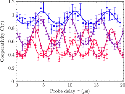
Figure 13: (Color online) Calibration of the Larmor frequency for different currents of the $B_{\mathrm{x}}$ coils. Shown is the cooperativity as a function of delay time $\tau$ for different transverse $B$-fields: $I_{\mathrm{x}}=10~{}\mathrm{mA}$ (blue squares), $I_{\mathrm{x}}=16~{}\mathrm{mA}$ (lilac stars), $I_{\mathrm{x}}=26~{}\mathrm{mA}$ (dark red circles), and $I_{\mathrm{x}}=36~{}\mathrm{mA}$ (red triangles). The solid lines are fits according to Eq. (30).

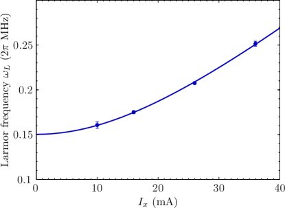
Figure 14: (Color online) Larmor frequency as a function of current through the $B_{\mathrm{x}}$ coils. The solid line is a fit of the form $\omega_{\mathrm{L}}=\sqrt{\omega_{\mathrm{z}}^{2}+a^{2}I_{\mathrm{x}}^{2}}$ and we deduce $\omega_{\mathrm{z}}=2\pi\times(0.150\pm 0.002)~{}\mathrm{MHz}$ and $\omega_{\mathrm{x}}=2\pi\times(5.5\pm 0.1)~{}\frac{\mathrm{kHz}}{\mathrm{mA}}\times I_{\mathrm{x}}$.

The amplitudes of the magnetic fields, $B_{\mathrm{x}}$ and $B_{\mathrm{z}}$, at the position of the ion crystal were calibrated by measuring the dependence of the Larmor frequency $\omega_{\mathrm{L}}$ with the intensity of the current used to drive the transverse magnetic field coils [see Eqs. (28) and (31)]. The obtained coupling as a function of $\tau$ is shown for different currents $I_{\mathrm{x}}$ on Fig. 13. The curves are fitted according to Eq. (30), yielding the individual Larmor frequencies. These frequencies are shown as a function of the current through the $B_{\mathrm{x}}$ coils in Fig. 14. Using the gyromagnetic ratio $\gamma_{\mathrm{GM}}=\frac{\mu_{\mathrm{B}}\mathfrak{g}_{3/2}}{\hbar}$ ($\mu_{\mathrm{B}}$ is the Bohr magneton, $\mathfrak{g}_{3/2}$ the Landé factor of the $3\mathrm{d}^{2}\mathrm{D}_{3/2}$ level), we deduce the magnetic fields along the two axis $B_{\mathrm{z}}=(0.134\pm 0.002)~{}\mathrm{G}$ and $B_{\mathrm{x}}=(4.91\pm 0.09)~{}\frac{\mathrm{G}}{\mathrm{A}}\times I_{\mathrm{x}}$.

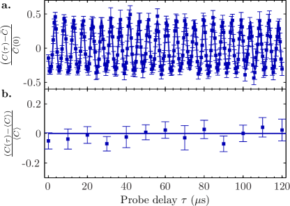
Figure 15: (Color online) (a) Normalized cooperativity paramter as a function of delay $\tau$. Due to the presence of a non-zero $B$-field component orthogonal to the quantization axis ($B_{\mathrm{z}}=B_{\mathrm{x}}=0.15~{}\mathrm{G}$), coherent Larmor precessions are observed. Long term drifts are compensated by normalizing to the mean of one oscillation period. The solid line corresponds to a fit, assuming an exponential decay and yields a coherence time of $\tau_{\mathrm{e}}=1.7^{100}_{-0.8}~{}\mathrm{ms}$. (b) Cooperativity as a function of delay with a $B$-field present only along the quantization axis ($B_{\mathrm{x}}=B_{\mathrm{y}}=0,~{}B_{\mathrm{z}}=0.15~{}\mathrm{G}$). The data points are normalized to the mean cooperativity of $\langle C\rangle=1.43\pm 0.02$.

To achieve a large contrast, the measurement was carried out with moderate $B$-field values $B_{\mathrm{x}}=B_{\mathrm{z}}=0.15~{}\mathrm{G}$ and the variation of the cooperativity was measured for $120~{}\mathrm{\mu s}$. To compensate for slow drifts during the measurement, each data point was normalized to the mean cooperativity, $\bar{C}$, averaged over one oscillation period. The normalized cooperativity is shown in Fig. 15(a), together with a fit of the form of (30), where decoherence processes are taken into account by multiplying the oscillating terms with an exponential decay term $\exp(-\nicefrac{{\tau}}{{\tau_{\mathrm{e}}}})$, which would be expected, e.g., for a homogeneous broadening of the energy levels. From this fit, we deduce a coherence time of $\tau_{\mathrm{e}}=1.7^{100}_{-0.8}~{}\mathrm{ms}$. This value is comparable to previously measured coherence times for single ions in linear Paul trap in equivalent magnetic field sensitive states Schmidt-Kaler2003 and might be further improved by an active control of stray magnetic fields or state configurations that are less magnetic field sensitive. For inhomogeneous broadening, due to magnetic field gradient over the crystal, the decoherence process would be better described by a Gaussian decay Chaneliere2005 . Fitting the data assuming a Gaussian decay $\exp(-\nicefrac{{\tau^{2}}}{{\tau_{\mathrm{g}}^{2}}})$ in Eq. (30) yields a coherence time of $\tau_{\mathrm{g}}=0.5_{-0.2}^{+0.6}~{}\mathrm{ms}$. Due to the limitation of our measurement to time delays of $\tau\lesssim 120~{}\mathrm{\mu s}$, it is at present not possible to distinguish between the two decay mechanisms.

For comparison, the cooperativity as a function of probe delay, $C(\tau)$, was measured with only the bias field along the quantization axis present ($B_{\mathrm{x}}=0,~{}B_{\mathrm{z}}=0.15\mathrm{G}$), as shown in Fig. 15 b. Here, the values are normalized to the mean cooperativity averaged over all points $\langle C\rangle$. Within the error bars, the deduced cooperativities agree with a constant value of $\langle C\rangle=1.43\pm 0.02$ (solid line).

VI Conclusion

To conclude, we have presented a detailed theoretical and experimental analysis of the experiments of Herskind2009Realization , which demonstrated the possibility of using large ion Coulomb crystals positioned in a moderately high-finesse optical cavity to enter the collective strong-coupling regime of CQED. The excellent agreement between the experimental results including those of Ref. Herskind2009Realization and the theoretical predictions, makes ion Coulomb crystals promising candidates for the realization of quantum information processing devices such as quantum memories and repeaters Duan2001 ; Kimble2008 . Using, for instance, cavity EIT-based protocols Fleischhauer2000 ; Lukin2000 ; Dantan2008c ; Gorshkov2007 ; Albert2011Cavity , the obtained coupling strengths and coherence times could open up for the realization of both high-efficiency and long life-time quantum memories Lvovsky2009Optical . Moreover, the nice properties of ion Coulomb crystals also allow for the manipulation of complex multimode photonic information Lvovsky2009Optical by exploiting the crystal spatial Dantan2009Large or motional Dantan2010Non-invasive degrees of freedom. Ion Coulomb crystals in optical cavities have also great potential for the investigation of cavity optomechanical phenomena Kippenberg2008 and the observation of novel phase transitions Garcia-Mata2007Frenkel-Kontorova ; Retzker2008Double ; Fishman2008Structural ; Harkonen2009Dicke ; Baumann2010Dicke with cold, solid-like objects.

We acknowledge financial support from the Carlsberg Foundation, the Danish Natural Science Research Council through the ESF EuroQUAM project CMMC, and the EU commission through the FP7 ITN project CCQED and STREP project PICC.

References

- (1) P. R. Berman, editor, Cavity Quantum Electrodynamics (Academic Press, London, 1994).
- (2) S. Haroche and J.-M. Raimond, Exploring the Quantum: Atoms, Cavities, and Photons (Oxford University Press, Oxford, 2006).
- (3) G. Rempe, R. J. Thompson, and H. J. Kimble, Phys. Scr. 1994, 67 (1994).
- (4) M. Brune, A. Maali, J. Dreyer, E. Hagley, J. M. Raimond, and S. Haroche, Phys. Rev. Lett. 76, 1800 (1996).
- (5) R. J. Thompson, G. Rempe, and H. J. Kimble, Phys. Rev. Lett. 68, 1132 (1992).
- (6) A. Badolato, K. Hennessy, M. Atatüre, J. Dreiser, E. Hu, P. M. Petroff, and A. Imamoğlu, Science 308, 1158 (2005).
- (7) G. Khitrova, H. M. Gibbs, M. Kira, S. W. Koch, and A. Scherer, Nature Phys. 2, 81 (2006).
- (8) A. Wallraff, D. I. Schuster, A. Blais, L. Frunzio, R.-S. Huang, J. Majer, S. Kumar, S. M. Girvin, and R. J. Schoelkopf, Nature (London) 431, 162 (2004).
- (9) I. Chiorescu, P. Bertet, K. Semba, Y. Nakamura, C. J. P. M. Harmans, and J. E. Mooij, Nature (London) 431, 159 (2004).
- (10) C. J. Hood, M. S. Chapman, T. W. Lynn, and H. J. Kimble, Phys. Rev. Lett. 80, 4157 (1998).
- (11) P. Maunz, T. Puppe, I. Schuster, N. Syassen, P. W. H. Pinkse, and G. Rempe, Phys. Rev. Lett. 94, 033002 (2005).
- (12) M. Harlander, M. Brownnutt, W. Hänsel, and R. Blatt, New J. Phys 12, 093035+ (2010).
- (13) P. F. Herskind, S. X. Wang, M. Shi, Y. Ge, M. Cetina, and I. L. Chuang, Opt. Lett. 36, 3045 (2011).
- (14) G. R. Guthohrlein, M. Keller, K. Hayasaka, W. Lange, and H. Walther, Nature 414, 49 (2001).
- (15) A. Kreuter, C. Becher, G. P. T. Lancaster, A. B. Mundt, C. Russo, H. Haffner, C. Roos, J. Eschner, F. Schmidt-Kaler, and R. Blatt, Phys. Rev. Lett. 92, 203002 (2004).
- (16) M. Keller, B. Lange, K. Hayasaka, W. Lange, and H. Walther, Nature (London) 431, 1075 (2004).
- (17) H. G. Barros, A. Stute, T. E. Northup, C. Russo, P. O. Schmidt, and R. Blatt, New J. Phys. 11, 103004+ (2009).
- (18) D. R. Leibrandt, J. Labaziewicz, V. Vuletić, and I. L. Chuang, Phys. Rev. Lett. 103, 103001+ (2009).
- (19) F. Dubin, C. Russo, H. G. Barros, A. Stute, C. Becher, P. O. Schmidt, and R. Blatt, Nature Phys. 6, 350 (2010).
- (20) Y. Kaluzny, P. Goy, M. Gross, J. M. Raimond, and S. Haroche, Phys. Rev. Lett. 51, 1175 (1983).
- (21) A. Lambrecht, T. Coudreau, A. M. Steinberg, and E. Giacobino, Europhys. Lett. 36, 93 (1996).
- (22) B. Nagorny, T. Elsässer, and A. Hemmerich, Phys. Rev. Lett. 91, 153003+ (2003).
- (23) H. W. Chan, A. T. Black, and V. Vuletić, Phys. Rev. Lett. 90, 063003+ (2003).
- (24) D. Kruse, C. von Cube, C. Zimmermann, and P. W. Courteille, Phys. Rev. Lett. 91, 183601+ (2003).
- (25) Z. Chen, J. G. Bohnet, S. R. Sankar, J. Dai, and J. K. Thompson, Phys. Rev. Lett. 106, 133601+ (2011).
- (26) F. Brennecke, T. Donner, S. Ritter, T. Bourdel, M. Köhl, and T. Esslinger, Nature (London) 450, 268 (2007).
- (27) Y. Colombe, T. Steinmetz, G. Dubois, F. Linke, D. Hunger, and J. Reichel, Nature (London) 450, 272 (2007).
- (28) P. F. Herskind, A. Dantan, J. P. Marler, M. Albert, and M. Drewsen, Nature Phys. 5, 494 (2009).
- (29) H. J. Kimble, Nature (London) 453, 1023 (2008).
- (30) A. Lambrecht, E. Giacobino, and J. M. Courty, Opt. Commun. 115, 199 (1995).
- (31) A. Joshi and M. Xiao, Phys. Rev. Lett. 91, 143904+ (2003).
- (32) P. Grangier, J. F. Roch, and G. Roger, Phys. Rev. Lett. 66, 1418 (1991).
- (33) J. F. Roch, , K. Vigneron, P. Grelu, A. Sinatra, J. P. Poizat, and P. Grangier, Phys. Rev. Lett. 78, 634 (1997).
- (34) S. L. Mielke, G. T. Foster, and L. A. Orozco, Phys. Rev. Lett. 80, 3948 (1998).
- (35) A. T. Black, J. K. Thompson, and V. Vuletić, Phys. Rev. Lett. 95, 133601+ (2005).
- (36) J. K. Thompson, J. Simon, H. Loh, and V. Vuletic, Science 313, 74 (2006).
- (37) J. Simon, H. Tanji, S. Ghosh, and V. Vuletic, Nature Phys. 3, 765 (2007).
- (38) H. Tanji, S. Ghosh, J. Simon, B. Bloom, and V. Vuletić, Phys. Rev. Lett. 103, 043601+ (2009).
- (39) V. Josse, A. Dantan, L. Vernac, A. Bramati, M. Pinard, and E. Giacobinoe, Phys. Rev. Lett. 91, 103601+ (2003).
- (40) V. Josse, A. Dantan, A. Bramati, M. Pinard, and E. Giacobino, Phys. Rev. Lett. 92, 123601+ (2004).
- (41) I. D. Leroux, M. H. Schleier-Smith, and V. Vuletić, Phys. Rev. Lett. 104, 073602+ (2010).
- (42) J. Klinner, M. Lindholdt, B. Nagorny, and A. Hemmerich, Phys. Rev. Lett. 96, 023002+ (2006).
- (43) S. Slama, S. Bux, G. Krenz, C. Zimmermann, and P. W. Courteille, Phys. Rev. Lett. 98, 053603+ (2007).
- (44) K. W. Murch, K. L. Moore, S. Gupta, and D. M. Stamper-Kurn, Nature Phys. 4, 561 (2008).
- (45) F. Brennecke, S. Ritter, T. Donner, and T. Esslinger, Science 322, 235 (2008).
- (46) A. T. Black, H. W. Chan, and V. Vuletić, Phys. Rev. Lett. 91, 203001+ (2003).
- (47) K. Baumann, C. Guerlin, F. Brennecke, and T. Esslinger, Nature (London) 464, 1301 (2010).
- (48) W. Lange, Nature Phys. 5, 455 (2009).
- (49) M. D. Lukin, S. F. Yelin, and M. Fleischhauer, Phys. Rev. Lett. 84, 4232 (2000).
- (50) L. M. Duan, M. D. Lukin, J. I. Cirac, and P. Zoller, Nature (London) 414, 413 (2001).
- (51) D. Leibfried, R. Blatt, C. Monroe, and D. Wineland, Rev. Mod. Phys 75, 281 (2003).
- (52) R. Blatt and D. Wineland, Nature (London) 453, 1008 (2008).
- (53) M. Drewsen, C. Brodersen, L. Hornekær, J. S. Hangst, and J. P. Schiffer, Phys. Rev. Lett. 81, 2878 (1998).
- (54) L. Hornekær and M. Drewsen, Phys. Rev. A 66, 013412+ (2002).
- (55) L. Hornekær, N. Kjærgaard, A. M. Thommesen, and M. Drewsen, Phys. Rev. Lett. 86, 1994 (2001).
- (56) A. Dantan, M. Albert, J. P. Marler, P. F. Herskind, and M. Drewsen, Phys. Rev. A 80, 041802+ (2009).
- (57) A. I. Lvovsky, B. C. Sanders, and W. Tittel, Nature Photon. 3, 706 (2009).
- (58) D. V. Vasilyev, I. V. Sokolov, and E. S. Polzik, Phys. Rev. A 77, 020302+ (2008).
- (59) K. Tordrup, A. Negretti, and K. Mølmer, Phys. Rev. Lett. 101, 040501+ (2008).
- (60) J. H. Wesenberg, Z. Kurucz, and K. Mølmer, Phys. Rev. A 83, 023826+ (2011).
- (61) D. H. E. Dubin, Phys. Rev. Lett. 66, 2076 (1991).
- (62) D. H. E. Dubin and J. P. Schiffer, Phys. Rev. E 53, 5249 (1996).
- (63) A. Dantan, J. P. Marler, M. Albert, D. Guénot, and M. Drewsen, Phys. Rev. Lett. 105, 103001+ (2010).
- (64) T. J. Kippenberg and K. J. Vahala, Science 321, 1172 (2008).
- (65) I. García-Mata, O. V. Zhirov, and D. L. Shepelyansky, Eur. Phys. J. D 41, 325 (2007).
- (66) A. Retzker, R. C. Thompson, D. M. Segal, and M. B. Plenio, Phys. Rev. Lett. 101, 260504+ (2008).
- (67) S. Fishman, G. De Chiara, T. Calarco, and G. Morigi, Phys. Rev. B 77, 064111+ (2008).
- (68) K. Härkönen, F. Plastina, and S. Maniscalco, Phys. Rev. A 80, 033841+ (2009).
- (69) H.-P. Breuer and F. Petruccione, The Theory of Open Quantum Systems (Oxford University Press, Oxford, 2007).
- (70) H. Kogelnik and T. Li, Appl. Opt. 5, 1550 (1966).
- (71) M. Scully and M. Zubairy, Quantum Optics (Cambridge University Press, Cambridge, 1997).
- (72) M. Tavis and F. W. Cummings, Phys. Rev. 170, 379 (1968).
- (73) M. G. Raizen, R. J. Thompson, R. J. Brecha, H. J. Kimble, and H. J. Carmichael, Phys. Rev. Lett. 63, 240 (1989).
- (74) P. Herskind, A. Dantan, M. B. Langkilde-Lauesen, A. Mortensen, J. L. Sørensen, and M. Drewsen, Appl. Phys. B 93, 373 (2008).
- (75) N. Kjærgaard, L. Hornekær, A. M. Thommesen, Z. Videsen, and M. Drewsen, Appl. Phys. B 71, 207 (2000).
- (76) A. Mortensen, J. J. T. Lindballe, I. S. Jensen, P. Staanum, D. Voigt, and M. Drewsen, Phys. Rev. A 69, 042502+ (2004).
- (77) R. W. P. Drever, J. L. Hall, F. V. Kowalski, J. Hough, G. M. Ford, A. J. Munley, and H. Ward, Appl. Phys. B 31, 97 (1983).
- (78) P. Herskind, Cavity Quantum Electrodynamics with Ion Coulomb Crystals, PhD thesis, The University of Aarhus, 2008.
- (79) L. Turner, Phys. Fluids 30, 3196 (1987).
- (80) P. F. Herskind, A. Dantan, M. Albert, J. P. Marler, and M. Drewsen, J. of Phys. B 42, 154008+ (2009).
- (81) F. Schmidt-Kaler, S. Gulde, M. Riebe, T. Deuschle, A. Kreuter, G. Lancaster, C. Becher, J. Eschner, H. Häffner, and R. Blatt, J. Phys. B 36, 623 (2003).
- (82) T. Chanelière, D. N. Matsukevich, S. D. Jenkins, S.-Y. Lan, T. A. B. Kennedy, and A. Kuzmich, Nature (London) 438, 833 (2005).
- (83) M. Fleischhauer, S. F. Yelin, and M. D. Lukin, Opt. Commun. 179, 395 (2000).
- (84) A. Dantan and M. Pinard, Phys. Rev. A 69, 043810 (2004).
- (85) A. V. Gorshkov, A. André, M. D. Lukin, and A. S. Sørensen, Phys. Rev. A 76, 033804 (2007).
- (86) M. Albert, A. Dantan, and M. Drewsen, Nature Photon. 5, 633 (2011).