Persistent currents in dipolar Bose-Einstein condensates confined in annular potentials

Abstract

We consider a dipolar Bose-Einstein condensate confined in an annular potential, with all the dipoles being aligned along some arbitrary direction. In addition to the dipole-dipole interaction, we also assume a zero-range hard-core potential. We investigate the stability of the system against collapse, as well as the stability of persistent currents as a function of the orientation of the dipoles and of the strength of the hard-core interaction.

I Introduction

Ultracold gases of bosonic and fermionic atoms have shown numerous fascinating effects. In some relatively recent experiments, it has become possible to create Bose-Einstein condensates of dipolar atoms Grie ; Fatt ; Veng ; Lu , and also to confine ultracold polar molecules Cosp ; Sosp . Dipolar gases may give rise to novel physics as compared to non-dipolar ones: unlike the usual hard-core potential, which describes the effective atom-atom interaction of non-dipolar atoms, the dipole-dipole interaction is anisotropic, nonlocal and it may be partly attractive and partly repulsive. For example, even when all the dipoles are aligned (under, e.g., the action of an electric or magnetic field, as we consider in the present study), the sign and the strength of the interaction may vary spatially, and can be tuned externally by changing the orientation of the applied field Bar ; Lah .

In some other recent experiments, toroidal trapping potentials have been realized experimentally Gup ; Ols ; Ryu ; Hen ; Les , where Bose-Einstein condensates of non-dipolar atoms were observed to support persistent currents Ryu . The realization of a dipolar Bose-Einstein condensate trapped in toroidal/annular potentials should therefore be feasible experimentally, as well. A condensate in such a topologically non-trivial confining potential is an ideal system for the investigation of various interesting phenomena, including superfluid properties, nonlinear effects, etc.

Theoretical studies of dipolar atoms trapped in toroidal potentials have been performed recently Aba10 ; Aba2 ; Zol11 . In Ref. Aba10 , Abad et al.  considered a three-dimensional trapping geometry and used the Gross-Pitaevskii mean-field approximation to investigate the ground-state and the rotational properties of a dipolar condensate for a fixed orientation of the dipoles, which was chosen to be on the plane of motion of the atoms (say, the $x$-$y$ plane). It was shown that if the dipoles are pointing along, e.g., the $x$ axis, there is a high concentration of them around the two points with coordinates $(x,y,z)=(0,\pm R,0)$, with $R$ being the mean radius of the torus, since around these two points the dipoles are predominantly oriented head-to-tail and therefore the interaction is mostly attractive. As we see below, the dipolar energy has two degenerate minima at these two points. As a result, as the strength of the dipolar interaction increases – with all the other parameters kept fixed – the density shows first two peaks around them. Eventually this two-fold symmetry is broken and the cloud concentrates around only one of them. If the dipolar interaction becomes strong enough, the gas collapses. In the same study it was also found that the gas supports metastable currents. In a more recent paper Aba2 the same authors demonstrated that this system exhibits Josephson oscillations and macroscopic quantum self-trapping. Finally, in Ref. Zol11 , Zöllner et al. considered quasi-one-dimensional motion of aligned dipolar atoms along a toroidal trap, assuming a very tight confinement in the transverse direction, and studied the few-body regime with the method of numerical diagonalization of the many-body Hamiltonian.

In the present study we consider a dipolar Bose-Einstein condensate confined in a (quasi-two-dimensional) annular trap, and assume that all the dipoles are aligned along some direction, forming an angle $\Theta$ with their plane of motion. In addition to the dipolar interaction, we consider a zero-range contact potential with strength $g$. Using the mean-field, Gross-Pitaevskii approximation we determine the absolute and/or local minima of the energy of the system for several values of $g$ and $\Theta$. We identify a collapsed phase, in which the system cannot support itself, and a stable one. Within the stable phase we also find a subphase in which the gas supports metastable, persistent currents.

Our results show that the boundaries between the different phases have a sinusoidal dependence on the angle $\Theta$, in agreement with a simple variational model that we present. The atomic density distribution that we find resembles that of the study by Abad et al. When the dipole moment is perpendicular to the plane of motion of the atoms the density is axially symmetric. As the angle is tilted, the density develops two maxima, and eventually the cloud concentrates around only one of these two maxima. We also find that, as observed in Ref. Aba10 for $\Theta=0$, even when the particle density is not circularly symmetric, the system may support persistent currents, provided that the atoms are not concentrated around a single density maximum. This behaviour is in a sense reminiscent of the case of purely contact interactions, where, if the ground-state density localizes, the system undergoes solid-body rotation and there is no metastability.

In what follows we first present our model in Sec. II. In Sec. III we investigate the stability of the system against collapse, and in Sec. IV the stability of persistent currents. Finally, in Sec. V we present our conclusions.

II Model

We consider a dipolar Bose-Einstein condensate at zero temperature, confined in an axially-symmetric potential

$$V({\bf r})=V_{r}({\bf r}_{\perp})+V_{z}(z)=\frac{1}{2}M\omega^{2}(r_{\perp}-R)^{2}+\frac{1}{2}M\omega_{z}^{2}z^{2},$$

where the $z$ direction is chosen to be the symmetry axis of the potential, and ${\bf r}_{\perp}$ is the position vector on the $x$-$y$ plane. Also, $\omega_{z}$ and $\omega$ are the frequencies of the confinement along the $z$ axis and along the direction perpendicular to it. We choose $\omega_{z}/\omega$ equal to 100, in order for $\hbar\omega_{z}$ to be much larger than all the other energy scales in the problem, in which case the motion is quasi-two-dimensional. Finally, we consider $R/a_{0}=4$, where $a_{0}=[\hbar/(M\omega)]^{1/2}$ is the oscillator length corresponding to $\omega$, and $M$ is the atomic mass. Under these conditions $V({\bf r})$ describes an annular potential with mean radius $R$ and width $\approx a_{0}$, as shown schematically in Fig. 1.

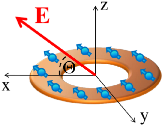
Figure 1: (Color online) Schematic illustration of the quasi-two-dimensional potential. A very tight confinement is assumed along the $z$ axis, while on the $x$-$y$ plane the atoms are assumed to move in an annulus of mean radius $R$ and width $\approx a_{0}$. The dipoles are oriented on the $x$-$z$ plane forming an angle $\Theta$ with the $x$ axis due to the action of an external (magnetic or electric) field ${\bf E}$.

Turning to the interactions, we consider both the usual contact potential and the dipole-dipole interaction,

$$V_{\rm int,3D}({\bf r},{\bf r}^{\prime})=U_{0}\delta({\bf r}-{\bf r}^{\prime})+D^{2}\frac{1-3\cos^{2}\theta_{rd}}{|{\bf r}-{\bf r}^{\prime}|^{3}},$$ (2)

where $U_{0}$ is the matrix element for zero-energy elastic atom-atom collisions. When the atoms have an electric dipole moment $d$, $D^{2}=d^{2}/(4\pi\epsilon_{0})$, where $\epsilon_{0}$ is the permittivity of the vacuum, while when the atoms have a magnetic moment $\mu$, $D^{2}=\mu_{0}\mu^{2}/(4\pi)$, where $\mu_{0}$ is the permeability of the vacuum. Finally, $\theta_{rd}$ is the angle between the dipole moment and the relative position vector ${\bf r}-{\bf r}^{\prime}$ of two dipoles.

The assumption of strong confinement along the $z$ axis implies that the motion of the atoms is frozen along this direction. This allows us to make an ansatz for the order parameter of the form $\Psi({\bf r})=Z(z)\Phi({\bf r}_{\perp})$, with $Z(z)=e^{-z^{2}/2a_{z}^{2}}/(\pi a_{z}^{2})^{1/4}$ being the ground state of the harmonic oscillator with frequency $\omega_{z}$, and $a_{z}=[\hbar/(M\omega_{z})]^{1/2}$. With this ansatz, one may integrate the dipole-dipole interaction along the $z$ direction and derive an effectively two-dimensional dipolar potential. After performing the integration, this potential takes the form Cre10

$$V_{\rm eff}({\bf r}_{\bot})=\frac{D^{2}}{\sqrt{8\pi}}\frac{e^{\tilde{r}_{\perp}^{2}}}{a_{z}^{3}}\biggl{\{}(2+4\tilde{r}_{\perp}^{2})K_{0}(\tilde{r}_{\perp}^{2})-4\tilde{r}_{\perp}^{2}K_{1}(\tilde{r}_{\perp}^{2})$$

$$+\cos^{2}\Theta\biggl{[}-(3+4\tilde{r}_{\perp}^{2})K_{0}(\tilde{r}_{\perp}^{2})+(1+4\tilde{r}_{\perp}^{2})K_{1}(\tilde{r}_{\perp}^{2})\biggl{]}$$

$$+2\cos^{2}\Theta\cos^{2}\phi\biggl{[}-2\tilde{r}_{\perp}^{2}K_{0}(\tilde{r}_{\perp}^{2})+(2\tilde{r}_{\perp}^{2}-1)K_{1}(\tilde{r}_{\perp}^{2})\biggl{]}\biggl{\}},$$ (3)

where $\phi$ is the angle in cylindrical polar coordinates, $\tilde{r}_{\perp}\equiv r_{\bot}/(2a_{z})$, and $K_{0}$ and $K_{1}$ are the zeroth-order and first-order modified Bessel functions of the second kind.

Integrating also the contact interaction over the $z$ direction we find that the total effective interaction is given by

$$V_{\rm int,2D}({\bf r}_{\bot})=g\delta({\bf r}_{\bot})+V_{\rm eff}({\bf r}_{\bot}),$$ (4)

where $g\equiv U_{0}\int|\phi_{0}(z)|^{4}dz=U_{0}/(\sqrt{2\pi}a_{z})$. Therefore, $\Phi({\bf r}_{\perp})$ satisfies the Gross-Pitaevskii-like equation

$$\biggl{[}-\frac{\hbar^{2}\nabla_{\bot}^{2}}{2M}+V_{r}({\bf r}_{\bot})+V_{\rm dip}({\bf r}_{\bot})+g|{\Phi({\bf r}_{\bot})}|^{2}\biggl{]}\Phi({\bf r}_{\bot})=$$

$$=\mu\Phi({\bf r}_{\bot}),$$ (5)

where $\mu$ is the chemical potential, and

$$V_{\rm dip}({\bf r}_{\bot})=\int V_{\rm eff}({\bf r}_{\bot}-{\bf r}_{\bot}^{\prime})\,\left|\Phi({\bf r}_{\bot}^{\prime})\right|^{2}\,d{\bf r}_{\bot}^{\prime}$$ (6)

is the effective dipolar interaction potential. In order to solve Eq. (5), we have employed a fourth-order split-step Fourier method within an imaginary-time propagation approach Chi05 . The method requires the selection of an initial state, which is then propagated in imaginary time until a (local or absolute) minimum of the energy is reached and numerical convergence is achieved. In what follows we fix the value of the dipolar length $a_{dd}\equiv MD^{2}/(3\hbar^{2})$, to the value of $a_{dd}/a_{0}=4/3$, and vary $\Theta$ and $g$.

III Stability of the ground state

We first investigate the ground state of the system. Since the dipolar interaction may be partly attractive, and we also allow for negative values of the contact interaction, we start with the stability of the ground state against collapse. For this purpose, we choose the initial guess for $\Phi({\bf r}_{\perp})$ to be proportional to $\exp[-(r_{\perp}-R)^{2}/2a_{0}^{2}]$, i.e., an axially symmetric Gaussian, which is peaked around $r_{\perp}=R$, with a width determined by $a_{0}$. For a given $\Theta$, we solve Eq. (5) for different values of $g$, identifying the different phases, and then we plot the corresponding phase diagram $g=g(\Theta)$, which is shown in Fig. 2.

The boundary separating the collapsed from the stable phase can be fitted rather well by the following sinusoidal function

$$g_{c,{\rm stab}}/g_{0}\approx 11.0\cos(2\Theta)-3.5,$$ (7)

with $g_{0}\equiv D^{2}/(4a_{z})$, which is represented by the dashed curve in Fig. 2. As expected, the minimum value of $g$ necessary to prevent the collapse decreases as the orientation angle of the dipoles $\Theta$ increases, since in this case the dipole-dipole interaction becomes increasingly repulsive.

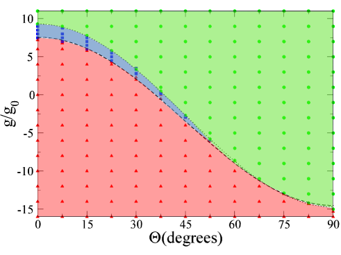
Figure 2: (Color online) Phase diagram with the orientation of the dipoles $\Theta$ in the horizontal axis and the strength of the contact potential $g$ in the vertical one. The three phases discussed in the text are presented: the stable phase where there exist metastable states (green circles), the stable phase that does not support persistent currents (blue squares), and the collapsed phase (red triangles). The dashed and dotted lines represent the fitting functions of Eqs. (7) and (11), respectively.

In order to get a better understanding of the above results, it is instructive to consider a variational order parameter of the form $\Psi({\bf r})=Z(z)\Phi_{\perp}(s_{\perp})\Phi_{l}(s_{l})$, where all the three functions are assumed to be Gaussian with widths determined by the oscillator length $a_{z}$, and the variational parameters $d_{\perp}$ and $d_{l}$ (as discussed in detail in the Appendix). Here $s_{\perp}$ is the coordinate that corresponds to the transverse direction and is measured from the minimum of the annular potential. Also, $s_{l}$ is the coordinate that corresponds to the longitudinal direction and is measured from one of the two minima of the dipolar interaction. As shown in the Appendix, we first integrate the dipole-dipole interaction entering Eq. (2) along the vertical and transverse directions, assuming $a_{z}\ll d_{\perp}$. Then, if we consider two dipoles located at the positions $s_{l}$ and $s_{l}^{\prime}$ along the annulus, for small values of $|s_{r}|\equiv|s_{l}-s_{l}^{\prime}|$, we obtain an effectively one-dimensional dipolar potential, which is given by

$$V_{d}(s_{l},s_{l}^{\prime})\approx\frac{\sqrt{8\pi}}{3\pi}\frac{ND^{2}}{d_{\perp}s_{r}^{2}}[1-3\sin^{2}(S/R)\cos^{2}\Theta].$$ (8)

As one can see, $V_{d}(s_{l},s_{l}^{\prime})$ separates in the relative coordinate $s_{r}=s_{l}-s_{l}^{\prime}$ and the center-of-mass coordinate $S=(s_{l}+s_{l}^{\prime})/2$, as in the case of quasi-one-dimensional motion in a toroidal trapping potential Meystre ; see also Refs. Santos ; Frank . In Eq. (8), the term that depends on the center-of-mass coordinate $S$ is $\propto 1-3\sin^{2}(S/R)\cos^{2}\Theta$, and has two degenerate local minima, at the points with coordinates $(x,y)=(0,\pm R)$, if $\Theta\neq 90^{\circ}$, as expected from the arguments presented earlier.

Integrating also in the longitudinal direction, under the assumption of a Gaussian profile, we find that the energy of the gas is

$$E \approx \left(\frac{\hbar^{2}}{2Ma_{z}^{2}}+\frac{1}{2}M\omega_{z}^{2}a_{z}^{2}\right)+\left(\frac{\hbar^{2}}{2Md_{\perp}^{2}}+\frac{1}{2}M\omega_{\perp}^{2}d_{\perp}^{2}\right)+$$

$$+ \frac{\hbar^{2}}{2Md_{l}^{2}}+\frac{Ng}{4\pi}\frac{1}{d_{l}d_{\perp}}+\frac{4}{3\pi}\frac{ND^{2}}{d_{l}d_{\perp}a_{z}}\left(1-\frac{3}{2}\cos^{2}\Theta\right).$$

In evaluating the last term we have introduced a cut-off length in the integration over $s_{r}$ set by the oscillator length $a_{z}$ in the $z$ direction. Also, the factor 3/2 in the same term comes from averaging the function $\sin^{2}(S/R)$ [that enters $V_{\rm CM}(S)$] along the longitudinal direction. This factor is accurate when $d_{l}$ is comparable to $R$, or in other words when the density in the longitudinal direction is either homogeneous, or close to homogeneous, as compared to the spatial variation of $V_{\rm CM}$, which is of the order of $R$.

Four important conclusions follow from Eq. (LABEL:trial):

(i) First of all, this problem resembles that of a non-dipolar system in two dimensions interacting via an effective contact potential with strength $g_{\rm eff}=g+{\cal C}D^{2}(1-3\cos^{2}\Theta/2)/a_{z}$, where ${\cal C}$ is a dimensionless constant of order unity.

(ii) If the motion in the transverse direction is frozen, the variational length $d_{\perp}$ may be set equal to the oscillator length $a_{0}$, and $d_{l}$ is the only free parameter. The motion is then quasi-one-dimensional and, for small values of $d_{l}$, the kinetic energy, which scales as $d_{l}^{-2}$, dominates over the interaction energy, which scales as $d_{l}^{-1}$. Thus, in this case the total energy is always bounded and there is no collapse. On the other hand, if the motion in the transverse direction is not frozen (i.e., as the annulus becomes wider), the system is not necessarily stable against collapse: in this case, the interaction energy scales as $(d_{l}d_{\perp})^{-1}$, and the kinetic energy scales as $d_{l}^{-2}$ and $d_{\perp}^{-2}$ along the longitudinal and the transverse directions, respectively. Therefore, the energy is not necessarily bounded and the system may collapse, under the conditions that we investigate below.

(iii) Provided that the system is stable, the energy has a local minimum that determines the width of the cloud in the transverse and longitudinal directions.

(iv) Finally, from Eq. (LABEL:trial) one may also deduce the functional form of the minimum value of $g(\Theta)$ that is necessary for the stability of the gas against collapse. Since $a_{z}$ is chosen to be small, the last two terms in Eq. (LABEL:trial) are the dominant ones. As a result, the critical value of $g$ is given by the approximate expression

$$\frac{g_{c,{\rm stab}}}{g_{0}}\approx\frac{16}{3}[3\cos(2\Theta)-1],$$ (10)

which is in rather good agreement with Eq. (7).

IV Persistent currents

We turn now to the second main question of the present study, which is the stability of persistent currents. To answer this question we choose the initial state to be proportional to $e^{im\phi}\exp[-(r_{\perp}-R)^{2}/2a_{\perp}^{2}]$, which has the same density distribution as before, but now with $m$ units of circulation. For a given value of $g$ and $\Theta$ (in the part of the phase diagram where the ground state is stable), the final state may or may not preserve the circulation, indicating the support or not of persistent currents for the particular choice of parameters. These two situations are represented in Fig. 2, with green circles and blue squares, respectively, for one unit of circulation, $m=1$. The boundary between these two phases is given approximately by

$${g_{c,{\rm met}}}/{g_{0}}\approx 12.0\cos(2\Theta)-2.7$$ (11)

and is represented in Fig. 2 by the dotted curve. In analogy to the case of non-dipolar atoms Bar10 , we have observed metastable states with up to four units of circulation, $m=4$ with the minimum value of $g$ necessary for the stability of the currents increasing with $m$.

Again, one can get some insight into this result from the variational model presented in the previous section. For a Bose-Einstein condensate with purely contact interactions that is confined in a ring potential, the critical value of $U_{0}$ for the existence of persistent currents with one unit of circulation satisfies the equation $n_{0}U_{0}/E_{\rm kin}=3/2$, where $E_{\rm kin}=\hbar^{2}/(2MR^{2})$ and $n_{0}$ is the density of the gas (homogeneously distributed) U ; GMK . Using this result for the effective coupling constant $g_{\rm eff}$, one gets

$$\frac{g_{c,{\rm met}}}{g_{0}}\approx\frac{16}{3}[3\cos(2\Theta)-1]-3\sqrt{2\pi}\,\frac{\hbar^{2}}{MR^{2}}\frac{Ra_{z}a_{\perp}}{ND^{2}}.$$ (12)

The above formula differs from Eq. (10) in the last term. However, this term is small, and therefore the variational model implies that $g_{c,{\rm met}}$ varies sinusoidally with $\Theta$, and also that the two phase boundaries are close to each other, in agreement with the numerical results.

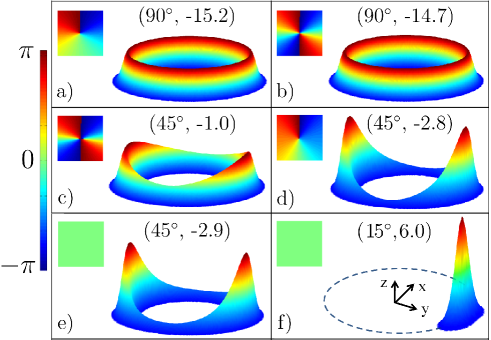
Figure 3: (Color online) Two-dimensional density distribution of the atoms, corresponding to different points $(\Theta,g/g_{0})$ of the phase diagram of Fig. 2. The phase of the order parameter for each configuration is also shown in the insets, with the associated colorbar represented on the left of the figure. Panels (a) and (d) correspond to metastable states with one unit of circulation, (b) and (c) to metastable states with two units of circulation, and (e), (f) correspond to current-free states. The dashed line in (f) is drawn to guide the eye along the minimum of the annular potential.

In Fig. 3 we show the two-dimensional density distribution and the phase of the order parameter corresponding to different values of $\Theta$ and $g/g_{0}$ within the blue and the green regions of the phase diagram of Fig. 2. When the dipole moment is oriented perpendicularly to the plane of motion of the atoms, the dipolar interaction is isotropic and purely repulsive, resembling the contact potential, and as a result the density is axially symmetric. Panels (a) and (b) show the density for $\Theta=90^{\circ}$ and $g/g_{0}=-15.2$ and $-14.7$, corresponding to metastable states with one and two units of circulation, respectively. Since the density is axially symmetric, the expectation value of the angular momentum per particle for these current-carrying states is $L/N=1$ and 2, respectively.

Panels (c), (d) and (e) show the density for $\Theta=45^{\circ}$ and $g/g_{0}=-1.0,-2.8$ and $-2.9$ respectively, corresponding to states with $m=2,1$, and 0. In this case, the dipolar interaction is anisotropic and as a result the cloud concentrates around two opposite ends of the annulus, as discussed earlier Aba10 . Notice that the states shown in (c) and (d) support persistent currents, even though the density is not axially symmetric. As a result, $L/N$ does not have an integer value and it is equal to $L/N=1.87$, 0.56 in panels (c) and (d), respectively.

Finally, in panel (f) we show the density for $\Theta=15^{\circ}$ and $g/g_{0}=6.0$. In this case there is a spontaneous symmetry-breaking due to the dipolar interaction and the density localizes in one of the two degenerate minima of the dipolar potential, in close analogy to the case of toroidal trapping Aba10 . The system then rotates as a solid body and persistent currents are not stable. Indeed, our results indicate that the presence of only one density maximum excludes the possibility of metastability.

V Summary and overview

In this study we have considered a dipolar Bose-Einstein condensate that is confined in an annular potential. The atoms are assumed to interact via the dipolar interaction, plus an extra short-ranged potential. The dipoles are assumed to be aligned along a direction that forms an angle $\Theta$ with their plane of motion. Our two basic results are the stability of the ground state against collapse and the stability of persistent currents as a function of the angle $\Theta$ and of the strength of the hard-core potential $g$.

The hard-core and the dipolar interactions combine, giving rise to an effective interaction that is spatially dependent. Furthermore, this effective interaction depends on the angle of orientation of the dipoles, which can be tuned externally by simply tilting the applied polarizing field. It is well known that the strength of the contact potential may be tuned via the so-called Feshbach resonances Wer05 . In our suggested physical system the tunability becomes possible via the change of the orientation of the external polarizing field. In addition, in the case of Feshbach resonances one may only change the value of the scattering length, while here the effective coupling is spatially dependent.

In the phase diagram $g$ versus $\Theta$ we determined two boundaries, one delimitating the region where the system is stable against collapse, and another one delimitating the region where persistent currents are stable. Both phase boundaries have a sinusoidal dependence on the angle $\Theta$, in agreement with a simple variational model that we have presented. As the strength of the dipolar interaction decreases, the variation of $g(\Theta)$ decreases and in the limit that it vanishes, the two phase boundaries which we have found become horizontal straight lines, corresponding to the limit of purely contact interactions.

We have seen that metastability of the flow is possible even for values of the angle $\Theta$ that give rise to inhomogeneous density distributions, provided that the gas preserves the two-fold symmetry of the dipolar interaction and is not concentrated around only one of the minima of the dipolar potential. According to our results, provided that the density is not homogeneous, the presence of two density maxima is a necessary, but not a sufficient condition for metastability. This situation is somewhat analogous to the case of a Bose-Einstein condensate which is trapped in a ring potential and interacts via purely contact interactions: in this case, if the strength of the contact potential is sufficiently large in magnitude and negative, there is a spontaneous symmetry breaking of the axial symmetry of the Hamiltonian. The ground-state density localizes and it is energetically favorable for the system to carry angular momentum via solid-body rotation, in which case the system does not support persistent currents.

An appealing property of this system is that one may sweep through all the three phases by simply changing the orientation angle of the dipoles, even when all the other parameters are kept fixed. An interesting potential application of this fact might be a “mesoscopic superfluid ring”, i.e., a device that is either “normal” or “superfluid”, depending on the orientation of the external polarizing field. Therefore, this problem is interesting not only for purely theoretical reasons, but also in connection with applications on e.g., precision measurements and nanotechnology.

VI Acknowledgements

We thank G. Bruun, J. Cremon and J. Smyrnakis for useful discussions. This work was financed by the Swedish Research Council. This project originated from a collaboration within the POLATOM Research Networking Programme of the European Science Foundation (ESF).

*

Appendix A Evaluation of the dipolar energy

The interaction between two dipoles with dipole moment $\bf d$ located at the positions ${\bf r}$ and ${\bf r}^{\prime}$ is given by

$$V_{\rm dip,3D}({\bf r},{\bf r}^{\prime})=D^{2}\frac{1-3\cos^{2}\theta_{rd}}{|{\bf r}-{\bf r}^{\prime}|^{3}},$$ (13)

where $\theta_{rd}$ is the angle between the relative position vector ${\bf r}-{\bf r}^{\prime}$ and ${\bf d}$. The relationship between $D$ and $d$ is given in Sec. II.

First we integrate over the vertical and transverse directions, assuming that the order parameter has a product form $\Psi({\bf r})=Z(z)\Phi_{\perp}(s_{\perp})\Phi_{l}(s_{l})$, with

$$Z(z)=\frac{1}{(\pi a_{z}^{2})^{1/4}}\,e^{-z^{2}/(2a_{z}^{2})},$$ (14)

$$\Phi_{\perp}(s_{\perp})=\frac{1}{(\pi d_{\perp}^{2})^{1/4}}\,e^{-s_{\perp}^{2}/(2d_{\perp}^{2})}.$$ (15)

The effective one-dimensional potential between two atoms which are located at the points $s_{l}$ and $s_{l}^{\prime}$ along the annulus is

$$V_{\rm dip,1D}(s_{l},s_{l}^{\prime})=\int V_{\rm dip,3D}({\bf r},{\bf r}^{\prime})\,|Z(z)|^{2}|\Phi_{\perp}(s_{\perp})|^{2}$$

$$\times|Z(z^{\prime})|^{2}|\Phi_{\perp}(s_{\perp}^{\prime})|^{2}\,dz\,ds_{\perp}\,dz^{\prime}\,ds_{\perp}^{\prime}.$$ (16)

Since the confinement along the $z$ direction is very tight, i.e., $a_{z}\ll d_{\perp}$, we consider for convenience the limit $a_{z}\to 0$. In this case,

$$\frac{1}{\sqrt{2\pi}\,a_{z}}\,e^{-z_{r}^{2}/(2a_{z}^{2})}\to\delta(z_{r}),$$ (17)

i.e., we get a delta function in the integration over the variable $z_{r}=z-z^{\prime}$. In this case $V_{\rm dip,1D}$ is given by the approximate expression

$$V_{\rm dip,1D}(s_{l},s_{l}^{\prime})=\frac{\sqrt{2\pi}}{4\pi}\frac{D^{2}}{d_{\perp}^{3}}\left[\frac{\sqrt{\pi}}{4{\tilde{s}}^{2}}U(3/2,0,2{\tilde{s}}^{2})+\right.$$

$$+\left.\frac{2}{3}(1-3\sin^{2}a)e^{{\tilde{s}}^{2}}\left[2{\tilde{s}}^{2}K_{0}({\tilde{s}}^{2})-(2{\tilde{s}}^{2}-1)K_{1}({\tilde{s}}^{2})\right]\right],$$

(18)

where $U$ is the confluent hypergeometric function, ${\tilde{s}}\equiv s_{r}/(2d_{\perp})$, with $s_{r}=s_{l}-s_{l}^{\prime}$ being the relative coordinate, and $\sin^{2}a\equiv\sin^{2}(S/R)\cos^{2}\Theta$.

Both for small and for large values of ${\tilde{s}}$ the term in the last line of Eq. (18) is the dominant one. For $|s_{l}-s_{l}^{\prime}|\gg d_{\perp}$ Eq. (18) reproduces the correct asymptotic behavior of the dipolar potential,

$$V_{\rm dip,1D}(s_{l},s_{l}^{\prime})\approx\frac{D^{2}}{s_{r}^{3}}(1-3\sin^{2}a).$$ (19)

Furthermore, for small values of $\tilde{s}$, Eq. (8) follows.

Assuming that the longitudinal wavefunction is also Gaussian,

$$\Phi_{l}(s_{l})=\frac{1}{(\pi d_{l}^{2})^{1/4}}\,e^{-s_{l}^{2}/(2d_{l}^{2})},$$ (20)

the dipolar energy $E_{d}$ of the system is given by

$$E_{d}=\int V_{\rm dip,1D}(s_{l},s_{l}^{\prime})\,|\Phi_{l}(s_{l})|^{2}|\Phi_{l}(s_{l}^{\prime})|^{2}\,ds_{l}\,ds_{l}^{\prime}.$$ (21)

Since the dominant contribution to this integral comes from small values of $\tilde{s}$, we use the expansion of $V_{\rm dip,1D}(s_{l},s_{l}^{\prime})$, given by Eq. (8) to find that

$$E_{d} \approx \frac{\sqrt{8\pi}}{3\pi}\frac{D^{2}}{d_{\perp}}(1-3\sin^{2}a)\int\frac{1}{s_{r}^{2}}\,|\Phi_{l}(s_{l})|^{2}|\Phi_{l}(s_{l}^{\prime})|^{2}\,ds_{l}\,ds_{l}^{\prime}$$ (22)

$$= \frac{4}{3\pi}\frac{ND^{2}}{d_{l}d_{\perp}a_{z}}\left(1-3\sin^{2}a\right).$$

In the integration over the relative coordinate $s_{r}$ we have introduced a cut-off, which we have set equal to $a_{z}$. This cut-off comes from the fact that in the derivation of the potential $V_{\rm dip,1D}(s_{l},s_{l}^{\prime})$ we have taken the limit of $a_{z}\to 0$, which gives a delta function in the integration over $z-z^{\prime}$. As a result, in the initial integration, where we have the term $(x-x^{\prime})^{2}+(y-y^{\prime})^{2}+(z-z^{\prime})^{2}$ in the denominator, we have set $z=z^{\prime}$. However, in the actual calculation $a_{z}$ is small but finite. To take this into account, we have replaced the lower limit of $s_{r}$ in the integration over this variable by the “width” of the delta function, or in other words with the average value of $\sqrt{\langle(z-z^{\prime})^{2}\rangle}$, which is $\sim a_{z}$.

References

- (1) A. Griesmaier, J. Werner, S. Hensler, J. Stuhler, and T. Pfau, Phys. Rev. Lett. 94, 160401 (2005).
- (2) M. Fattori, G. Roati, B. Deissler, C. D’Errico, M. Zaccanti, M. Jona-Lasinio, L. Santos, M. Inguscio, and G. Modugno, Phys. Rev. Lett. 101, 190405 (2008); S. E. Pollack, D. Dries, M. Junker, Y. P. Chen, T. A. Corcovilos, and R. G. Hulet, ibid. 102, 090402 (2009).
- (3) M. Vengalattore, S. R. Leslie, J. Guzman, and D. M. Stamper-Kurn, Phys. Rev. Lett. 100, 170403 (2008).
- (4) M. Lu, S. H. Youn, and B. L. Lev, Phys. Rev. Lett. 104, 063001 (2010).
- (5) C. Ospelkaus, S. Ospelkaus, L. Humbert, P. Ernst, K. Sengstock, and K. Bongs, Phys. Rev. Lett. 97, 120402 (2006).
- (6) S. Ospelkaus, A. Pe’er, K.-K. Ni, J. J. Zirbel, B. Neyenhuis, S. Kotochigova, P. S. Julienne, J. Ye, and D. S. Kin, Nat. Phys. 4, 622 (2008).
- (7) M. A. Baranov, Phys. Rep. 464, 71 (2008).
- (8) T. Lahaye, C. Menotti, L. Santos, M. Lewenstein, and T. Pfau, Rep. Prog. Phys. 72, 126401 (2009).
- (9) S. Gupta, K. W. Murch, K. L. Moore, T. P. Purdy, and D. M. Stamper-Kurn, Phys. Rev. Lett. 95, 143201 (2005).
- (10) S. E. Olson, M. L. Terraciano, M. Bashkansky, and F. K. Fatemi, Phys. Rev. A 76, 061404(R) (2007).
- (11) C. Ryu, M. F. Andersen, P. Clad´e, V. Natarajan, K. Helmerson, and W. D. Phillips, Phys. Rev. Lett. 99, 260401 (2007).
- (12) K. Henderson, C. Ryu, C. MacCormick, and M. G. Boshier, New J. Phys. 11, 043030 (2009).
- (13) I. Lesanovsky and W. von Klitzing, Phys. Rev. Lett. 99, 083001 (2007).
- (14) M. Abad, M. Guilleumas, R. Mayol, M. Pi, and D. M. Jezek, Phys. Rev. A 81, 043619 (2010).
- (15) M. Abad, M. Guilleumas, R. Mayol, M. Pi, and D. M. Jezek, Europh. Phys. Lett. 94, 10004 (2011).
- (16) S. Zöllner, G. M. Bruun, C. J. Pethick, and S. M. Reimann, Phys. Rev. Lett. 107, 035301 (2011).
- (17) J. C. Cremon, G. M. Bruun, and S. M. Reimann, Phys. Rev. Lett. 105, 255301 (2010).
- (18) S. A. Chin and E. Krotscheck, Phys. Rev. E 72, 036705 (2005).
- (19) O. Dutta, M. Jääskeläinen, and P. Meystre, Phys. Rev. A 73, 043610 (2006).
- (20) S. Sinha and L. Santos, Phys. Rev. Lett. 99, 140406 (2007).
- (21) F. Deuretzbacher, J. C. Cremon, and S. M. Reimann, Phys. Rev. A 81, 063616 (2010).
- (22) S. Bargi, F. Malet, G. M. Kavoulakis, and S. M. Reimann, Phys. Rev. A 82, 043631 (2010).
- (23) R. Kanamoto, H. Saito, and M. Ueda, Phys. Rev. A 68, 043619 (2003).
- (24) G. M. Kavoulakis, Phys. Rev. A 69, 023613 (2004).
- (25) J. Werner, A. Griesmaier, S. Hensler, J. Stuhler, T. Pfau, A. Simoni, and E. Tiesinga, Phys. Rev. Lett. 94, 183201 (2005).