Application of Self-Organizing Map to stellar spectral classifications

Abstract

We present an automatic, fast, accurate and robust method of classifying astronomical objects. The Self Organizing Map (SOM) as an unsupervised Artificial Neural Network (ANN) algorithm is used for classification of stellar spectra of stars. The SOM is used to make clusters of different spectral classes of Jacoby, Hunter and Christian (JHC) library. This ANN technique needs no training examples and the stellar spectral data sets are directly fed to the network for the classification. The JHC library contains 161 spectra out of which, 158 spectra are selected for the classification. These 158 spectra are input vectors to the network and mapped into a two dimensional output grid. The input vectors close to each other are mapped into the same or neighboring neurons in the output space. So, the similar objects are making clusters in the output map and making it easy to analyze high dimensional data.

After running the SOM algorithm on 158 stellar spectra, with 2799 data points each, the output map is analyzed and found that, there are 7 clusters in the output map corresponding to O to M stellar type. But, there are 12 misclassifications out of 158 and all of them are misclassified into the neighborhood of correct clusters which gives a success rate of about 92.4%.

1 Introduction

Artificial neural networks are now becoming a more popular tools for handling astronomical data. It is very important to have some automatic means of analyzing large databases like the surveys and upcoming space missions which would release terabytes of data to the community. That is why, ANNs are widely used as an automatic tools for analyzing astronomical data. Some of the previous attempts on ANNs in astronomy are: Gulati et al. (1994, 1995) ,Von Hippel et al. (1994) ,Weaver et al. (1995) ,Singh et al. (1998, 2003) , Gupta et al. (2004), Allende Prieto, C. (2004), Bazarghan et al. (2008) ,Bazarghan M. (2008), Bazarghan, M., Gupta, R. (2008), Wyrzykowski and Belokurov (2008).

Artificial neural network techniques used in the field of astronomy have been mostly supervised algorithms. Here we introduce an application of unsupervised technique to identify different classes of objects and try to make a cluster of similar type of stars using this technique.

The Jacoby, Hunter and Christian (1984) library is used for classification using SOM algorithm as unsupervised ANN. This algorithm configures output into a topological presentation of the original multi-dimensional data, producing a SOM in which input vectors with similar features are mapped to the same map unit or nearby units. In this way at the output map we will have the clusters of similar objects at different positions of the map. The expected clusters in this case are the stellar spectral type ranging from O to M.

The Self- Organizing Map algorithm is explained in section 2 . In section 3 we describe the input data and their preprocessing. The result of classification and discussion are presented in sections 4 and 5 respectively.

2 Self-Organizing Map

Self-Organizing Map neural net developed by Kohonen, T. (1981a); Kohonen, T (1981b, c, d, 1982a, 1982b) is important from many point of view as it pays attention to spatial order unlike the traditional neural models and that is why this technique acquired a very special position in neural network theory. The following section is the description of this technique in details.

Neural network learning is not restricted to supervised learning, wherein training pairs are provided, that is, input and target output pairs. A second major type of learning for neural network is unsupervised learning, in which the net seeks to find patterns or regularities in the input data. Self-Organizing Map (SOM), developed by Kohonen, groups the input data clusters, a common use for unsupervised learning. The adaptive resonance theory networks, are also clustering type networks.

Figure 1: Self-Organizing Map architecture, $m_{i}$ is the assigned weight vector of the unit on the map

Self-organizing map consists of two layers: A one dimensional input layer and a two dimensional competitive layer, organized as a 2D grid of units as shown in the Figure 1. SOM lattice structure composed of $N\times N$ neural units. This layer can neither be called hidden nor an output layer. Each input is connected to all output neurons in the map. A weight vector with the same dimensionality as the input vectors is attached to every neuron in the map.

The learning algorithm for the SOM accomplishes two important things:

1. Clustering the input data

2. Spatial ordering of the map so that input patterns tend to produce a response in units that are close to each other in the grid.

Since every unit in the competitive layer represents a cluster, the number of clusters that can be formed, will be limited by the number of units in the competitive layer.

The weight vector for a competitive layer unit in a clustering net serves as a representative, exemplar, or codebook vector for the input patterns, which the net has placed on that cluster. While training, the net determines the output units that is the best match for the current input vector; then the weight vector of the winner is adjusted according to net’s learning algorithm.

The beauty of the self-organizing maps is their ability to find regularities and correlations in the input layer and group them into vectors without any external adjustment or prior knowledge of the expected outcomes. Kohonen’s SOM is one of the most referenced mapping techniques because of its ability to flatten high dimensional input into two or three dimensional data. One of the most important attribute of Kohonen’s SOM is that, it does data compression without loss to relative distance between data points. The neurons are connected to adjacent neuron by a neighborhood relation, which decides the topology, or structure, of the map. The Figure 2 shows the rectangular and hexagonal lattice structures and their discrete neighborhoods (size 0,1 and 2) of the centermost unit.

Figure 2: rectangular and hexagonal lattice structures

The SOM is trained iteratively. In each training step one vector $x$ from the input data set is randomly chosen and then the distance between this vector and all the weight vectors of the map will be calculated and this distance measurement, typically is an Euclidian distance.

The neuron in the map whose weight vector is closest to the input vector, $x$, is called Best-Matching Unit (BMU), here denoted by c:

$$\parallel x-m_{c}\parallel=\min_{i}{\parallel x-m_{i}\parallel},\forall i=1,2,...,N\times N$$ (1)

After finding the BMU, the weight vector of the map are updated such that the BMU is moved closer to the input vector in the input space. The topological neighbors of the BMU are treated similarly. This process of adaptation of weight vectors intern moves the BMU and its topological neighbors towards the input sample vector $x$. The updating scheme aims at performing a stronger weight adaptation at the BMU location than in its neighborhood. This update rule in SOM for the weight vector of i is:

$$m_{i}(t+1)=m_{i}(t)+\alpha(t)h_{ci}(t)[x(t)-m_{i}(t)],$$ (2)

where $t$ presents the time, $x(t)$ is randomly chosen an input vector from the input data set at time $t$, $h_{ci}(t)$ is the neighborhood kernel around the ${\it winner}$ unit $c$ and $\alpha(t)$ is the learning rate at time $t$. The function $h_{ci}(t)$ has a very important role; it is defined over the lattice points. To achieve convergence it is necessary that $h_{ci}(t)\longrightarrow 0$ as t$\longrightarrow\infty$. Classically, a Gaussian function is used, leading to :

$$h_{ci}=exp-\frac{\parallel r_{c}-r_{i}\parallel^{2}}{2\delta(t)^{2}}$$ (3)

Here, the Euclidian norm is chosen and $r_{i}$ is the 2D location for the $i^{th}$ neuron in the network. $\delta(t)$ specifies the width of the neighborhood during time $t$.

The learning rate $\alpha$ must always be selected much less than 1, typically at most 0.4. Best results are usually achieved by slowly decreasing it as training progresses, the radius of the neighborhood around a cluster unit (winner) also decreases as the clustering process progresses, this decreasing of the learning rate and radius of neighborhood must be monotonic for better performance of the network. Up to a point, large learning rate will indeed make training process faster. If the learning rate selected to be very large then convergence may never occur, and in this case weight vector may oscillate highly and it can lead to instability.

3 The Input Data

The Jacoby, Hunter and Christian (1984) library is used as a data set for the classification and input to the SOM network. The JHC library covers the wavelength range of 3510-7427.2 Å  for various O to M stellar type and luminosity classes V, III, and I. This library contains 161 spectra of individual stars, we selected 158 of them as an input to the SOM classifier. The JHC library has a resolution of 4.5 Å  with one sample per 1.4 Å .

Each spectrum of this library is having 2799 number of data points and they are normalized to the unity before feeding into the network. The SOM technique is actually mapping 2799 dimensional data into two dimensional output map.

The 158 input spectra are labled as the JHC’s Atlas list, specifying their spectral, subspectral and luminosity types. These lables are require while analysing the output map. The lables are placed beside every node (neuron) on the output map which indicates, that specific neuron is activated by the corresponding input spectra. Hence we can point out the location of each input spectra in the map and study the behavior of the network in making clusters of similar spectral type.

4 Self-Organizing Map as a classifier

In this work the classification of the library of stellar spectra, Jacoby, Hunter and Christian (1984) using unsupervised artificial neural network, Self-Organizing Map algorithm (SOM) is presented.

The 158 spectra of the JHC library with 2799 data points each, are the input vectors of the network and mapped into two dimensional output grid. A problem with large SOMs is that when the map size is increased, the time it takes to do any operations on the map increases linearly. When the grid size becomes very large, finding the best matching unit takes longer and longer. The size of the SOM determines the resolution of the visualization it produces. On a small SOM, lots of data samples will be projected to each SOM unit, whereas on a large SOM the similarity relationships of the samples are more readily visible. The user must select the map size in advance. This may lead to many experiments with different sized maps, trying to obtain the optimal result. Different map size and itterations are tried out and their performances analysed some of which are given in Table 1. The map size of the $13\times 13$ with highest performance is selected for detailed analysis.

Table 1: List of Map sizes with number if itterations and their performances

Map size	No. of itterations	Performance
$7\times 7$	10000	87.34%
$9\times 9$	20000	84.17%
$11\times 11$	10000	82.27%
$13\times 13$	10000	92.4%
$15\times 15$	10000	89.87%
$17\times 17$	18000	81.64%
$19\times 19$	20000	81.01%

The 158 JHC spectral library are labeled with their true class given in the Jacoby, Hunter and Christian (1984). The Self-Organizing Map that finds the similarity and regularities in the input patterns, group them into clusters. Every neuron in the grid holds a weight (reference) vector, the closest neuron in the map to the input vector will win the competition. If a particular neuron represents a given pattern, then its neighbour represent similar patterns. This is because more than one neuron are allowed to learn from each presentation. The learning rate for neighbours is less than that for the winner, so their weights change less.

After inputing all 158 labled stellar spectra of JHC library to the network and completion of the learning process by Neural Network, the output map is generated. By visualizing the output map, we see that the spectrum labels are spread out on the map by sitting on different neurons as shown in the Figure 3.

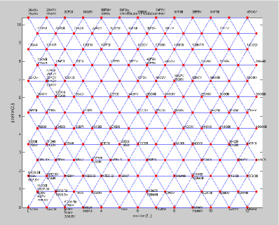
Figure 3: Kohonen output map for 158 labled JHC stellar spectra of stars as input

As we see in the output map some neurons are activated with single pattern, some with multiple patterns and some neurons have not been activated by any spectra. The output map is also presented in another format in Figure 4 which is called hit map. This map displays the number of hits in the form of shadowed hexagons and also lables expressing digitally the number of hits.

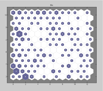
Figure 4: Number of hits indicated by shadowed sizes of the hexagons and also numbers printed inside each hexagon

This visualization method gives the number of hits (number of spectra that activates the node) for each node. The spectrum which activate single neuron are expected to be of the same class.

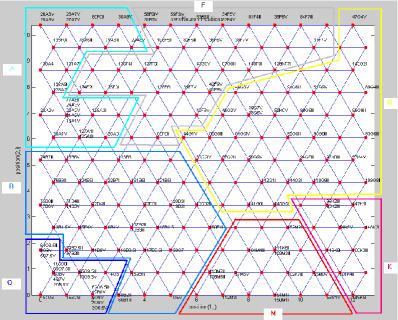
Figure 5: Kohonen output map showing labled clusters of spectral kind

The next step was to check the classification result and performance of the Self-Organizing Map. We can find out the clusters and groupings by referring to the labels in the map. The map is easily readable because of the presence of lables in the map and their position. If any input vector out of 158 spectra activates a neuron, its lable will be printed beside that winer neoron.

The performance of the network can be justified by simply looking at the generated Kohonen output map and cheking the cluster formation throughout the map. The Figure 5 shows the output for $13\times 13$ sized map with cluster and groupings of spectral types which are very nicely separated and located in different positions of the map. The clusters for the spectral types O - B - A - F - G - K and M are distinctly shown and separated by closed loops.

Further investigation on classification result was done to check misclassifications, and it is graphically presented in Figure 6.

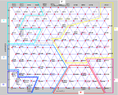
Figure 6: Kohonen output map showing misclassified patterns indicated with circles around the lables

Misclassified patterns are shown with circles around the lables inside the clusters. By looking at the clusters inside the specified boundry for every spectral type we can make out the wrongly classified and placement of the patterns. There are 12 misclassified patterns out of 158 spectra and all of them are misclassified into their neighbouring clusters as seen in Figure 6 which is success rate of about 92.4%.

The Table 2 shows the spectrum which are misclassified and their true class types.

Table 2: List of spectra classified wrongly

Misclassified pattern	Classified as	True class
12B0V	O	B
1O5V	B	O
158O7I	B	O
133F0I	A	F
80F0III	A	F
43G0V	F	M
87G0III	F	M
52K0V	G	K
97K0III	G	K
53K4V	G	K
111K6II	M	K
102K7III	M	K

5 Discussions

As it is seen from Table 2 and Figure 6 misclassified patterns belong to their neighboring clusters. For example 12B0V which is misclassified as O spectral type, is at the neighburhood of its true class. Likewise if we check all the misclassified patterns, we see that they are misclassified to their neighbouring true classes. The JHC libraray is very detailed and it also includes the subspectral types from 0-9. The misclassified patterns could be looked in detail to consider the subspectral types as well. It is found that the misclassified patterns are very close to their true class. for example, 80F0III is wrongly classified as spectral type A, but it is close to the neighbouring class, 30A9V. This is true with most of the misclassified patterns and it shows that the classification accuracy can be higher than 92.4%.

This technique and algorithm can be used for even larger unknown set of stellar spectra. Specially where we have different astronomical objects and need a pre-classification to identify the object types first, and then do further analysis on each cluster. The beauty of this algorithm is that we don’t need any exemplars to train the network but it finds the similarities by its own without any supervision and makes the clusters of similar objects.

6 Acknowledgments

The author wishes to thank Lukasz Wyrzykowski for his constructive comments.

References

- Allende Prieto, C. (2004) Allende Prieto, C. 2004, AN, 325, No. 6-8, 604
- Bazarghan et al. (2008) Bazarghan M.; Safari H.; Innes D. E.; Karami E.; Solanki S. K. 2008, A&A, 492, L13-L16.
- Bazarghan M. (2008) Bazarghan Mahdi 2008, Bull. Astr. Soc. India, 36, 1-54
- Bazarghan, M., Gupta, R. (2008) Bazarghan, M., Gupta, R. 2008, Astrophysics & Space Sci. 315, 201-210
- Gulati et al. (1994) Gulati, R. K.; Gupta, R.; Khobragade, S. 1994, ApJ, 426, 340
- Gulati et al. (1995) Gulati, R. K.;Gupta, R.; Khobragade, S. 1995, Astronomica Data Analysis Software and Systems IV, ASP Conf. Ser. vol. 77, R. A. Shaw, H.E. Payne,and J.J.E. Hayes, eds. p.253
- Gupta et al. (2004) Gupta, Ranjan; Singh, Harinder P.; Volk, K.; Kwok, S. 2004, ApJS, 152, 201
- Jacoby, Hunter and Christian (1984) Jacoby G. H., Hunter D A. and Christian C. A. 1984, ApJS, 56, 257-281
- Kohonen, T. (1981a) Kohonen, T., 1981, In Oja, E. and Simula, O., editors, Proceedings of 2SCIA, Scand Conference on Image Analysis, pages 214-220, Helsinki, Finland.
- Kohonen, T (1981b) Kohonen, T., 1981, Technical Report TKK-F-A 463, Helsinki: University of Technology, Espoo, Finland.
- Kohonen, T (1981c) Kohonen, T., 1981, Report TKK-F-A 461, Helsinki: University of Technology, Espoo, Finland.
- Kohonen, T (1981d) Kohonen, T., 1981, Report TKK-F-A 450, Helsinki: University of Technology, Espoo, Finland.
- Kohonen, T (1982a) Kohonen, T., 1982, Biological Cybernetics, 44(2):135-140.
- Kohonen, T (1982b) Kohonen, T., 1982, Biological Cybernetics, 43(1): 59-69.
- Singh et al. (1998) Singh, Harinder P.; Gulati, Ravi K.; Gupta, Ranjan. 1998, MNRAS, 295, 312
- Singh et al. (2003) Singh, Harinder P.; Gupta, Ranjan. 2003, Large Telescopes and Virtual Observatory: Visions for the Future, 25th meeting of the IAU, Joint Discussion 8.
- Von Hippel et al. (1994) Von Hipple, T.; Storrie-Lombardi,L. J.; Storrie-Lombardi,M. C.; Irwin,M. J. 1994, MNRAS, 269, 97
- Weaver et al. (1995) Weaver, Wm. Bruce; Torres-Dodgen, Ana V. 1995, ApJ, 446, 300
- Wyrzykowski and Belokurov (2008) Wyrzykowski, L. and Belokurov, V. “Classification and Discovery in Large Astronomical Surveys”meeting, Ringberg Castle, 2008, arXive:0811.1808