A Kalman Decomposition for Possibly Controllable Uncertain Linear Systems

Abstract

This paper considers the structure of uncertain linear systems building on concepts of robust unobservability and possible controllability which were introduced in previous papers. The paper presents a new geometric characterization of the possibly controllable states. When combined with previous geometric results on robust unobservability, the results of this paper lead to a general Kalman type decomposition for uncertain linear systems which can be applied to the problem of obtaining reduced order uncertain system models.

1 Introduction

Controllability and observability are fundamental properties of a linear system; e.g., see [1]. This paper is concerned with extending these notions to the case of uncertain linear systems with the aim of gaining greater understanding of the structure of uncertain linear systems when applied to problems of reduced order modelling and minimal realization.

One reason for considering the issue of controllability for uncertain systems might be to determine if a robust state feedback controller can be constructed for the system; e.g., see [2]. In this case, one would be interested in the question of whether the system is “controllable” for all possible values of the uncertainty; e.g., see [3, 4, 5, 6, 7, 8]. Similarly, one reason for considering observability for uncertain systems might be to determine if a robust state estimator can be constructed for the system; e.g., see [9]. In this case, one would be interested in the question of whether the system is “observable” for all possible values of the uncertainty; e.g., see [10]. However, these questions of robust controllability and robust observability are not the questions being addressed in this paper.

For the case of linear systems, the notions of controllability and observability are central to realization theory; e.g., see [1]. For example, it is known that if a linear system contains unobservable or uncontrollable states, those states can be removed in order to obtain a reduced dimension realization of the system’s transfer function. From this point of view, a natural extension of the notion of controllability to the case of uncertain systems, would be to consider “possibly controllable” states which are controllable for some possible values of the uncertainty. This idea was developed in the paper [11] for the case of uncertain linear systems with structured uncertainty subject to averaged integral quadratic constraints (IQCs). Similarly, a natural extension of the notion of observability to uncertain systems is to consider robustly unobservable states which are “unobservable” for all possible values of the uncertainty. This idea was developed in the papers [12, 13].

This paper builds on concepts of “robust unobservability and “possible controllability” developed in the papers [12, 11]. The results presented in the paper aim to provide insight into the structure of uncertain systems as it relates to questions of realization theory and reduced dimension modelling for uncertain systems; e.g., see [14, 15, 16].

We formally define notions of robust unobservability and possible controllability in terms of certain constrained optimization problems. The notion of robust unobservability used in this paper involves extending the standard linear systems definition of the observability Gramian to the case of uncertain systems; see also [17]. Also, the notion of possible controllability used in this paper involves extending the standard linear systems definition of the controllability Gramian to the case of uncertain systems; see also [18]. We then apply the S-procedure (e.g., see [2]) to obtain conditions for robust unobservability and possible controllability in terms of unconstrained LQ optimal control problems dependent on Lagrange multiplier parameters as in [12, 11]. From this, we develop a geometric characterization for the set of robustly unobservable states (as in [13]) and the set of possibly controllable states. These characterizations imply that the set of robustly unobservable states is in fact a linear subspace. Similarly, we show that the set of possibly controllable states is a linear subspace; see also [3, 6, 7]. These characterizations lead to a Kalman type decomposition for the uncertain systems under consideration; see also [19], [20] and Theorem 4.3 in Chapter 3 of [1]. This decomposition is described in the four possible cases for which an uncertain system model can have robustly unobservable states or states which are not possibly controllable. These are the cases in which a reduced dimension uncertain system model can be obtained which retains the same set of input-output behaviours as the original model. As compared to the previous papers [12, 13, 11], the results of this paper enable a complete geometrical picture to be obtained which can be applied to problems of reduced dimension modelling of uncertain linear systems. Also, the results of this paper are much more computationally tractable than the results of the papers [12, 11]. The main assumption required in this paper as compared to the previous papers [12, 11] is the assumption that the uncertainty is unstructured and described by a single averaged uncertainty constraint.

The remainder of the paper proceeds as follows. In Section 2, the class of uncertain systems under consideration is introduced and definitions of robust unobservability and possible controllability are given. In Section 3, the existing geometrical results on robust observability are summarized. In Sections 4, 5, 6, our main results on possible controllability are given. In Section 7, the results are combined to obtain complete Kalman decomposition results and in Section 8, an illustrative example is given. The paper is concluded in Section 9.

2 Problem Formulation

We consider the following linear time invariant uncertain system:

$$\dot{x}(t) = Ax(t)+B_{1}u(t)+B_{2}\xi(t);$$

$$z(t) = C_{1}x(t)+D_{1}u(t);$$

$$y(t) = C_{2}x(t)+D_{2}\xi(t)$$ (1)

where $x\in{\bf R}^{n}$ is the state, $y\in{\bf R}^{l}$ is the measured output, $z\in{\bf R}^{h}$ is the uncertainty output, $u\in{\bf R}^{m}$ is the control input, and $\xi\in{\bf R}^{r}$ is the uncertainty input.

For the system (2), we define the transfer function $G(s)$ to be the transfer function from the input $\xi(t)$ to the output $y(t)$; i.e.,

$$G(s)=C_{2}(sI-A)^{-1}B_{2}+D_{2}.$$

Also, we define the transfer function $H(s)$ to be the transfer function from the input $u(t)$ to the output $z(t)$; i.e.,

$$H(s)=C_{1}(sI-A)^{-1}B_{1}+D_{1}.$$

System Uncertainty. The uncertainty in the uncertain system (2) is required to satisfy a certain “Averaged Integral Quadratic Constraint”.

Averaged Integral Quadratic Constraint. Let the time interval $[0,~{}T]$, $T>0$ be given and let $d>0$ be a given positive constant associated with the system (2); see also [21, 12, 11]. We will consider sequences of uncertainty inputs ${\mathcal{S}}=\{\xi^{1}(\cdot),\xi^{2}(\cdot),\ldots\xi^{q}(\cdot)\}$. The number of elements $q$ in any such sequence is arbitrary. A sequence of uncertainty functions of the form ${\mathcal{S}}=\{\xi^{1}(\cdot),\xi^{2}(\cdot),\ldots\xi^{q}(\cdot)\}$ is an admissible uncertainty sequence for the system (2) if the following conditions hold: Given any $\xi^{i}(\cdot)\in{\mathcal{S}}$ and any corresponding solution $\{x^{i}(\cdot),\xi^{i}(\cdot)\}$ to (2) defined on $[0,T]$, then $\xi^{i}(\cdot)\in{\bf L}_{2}[0,T]$, and

$$\frac{1}{q}\sum_{i=1}^{q}\int_{0}^{T}\left(\|\xi^{i}(t)\|^{2}-\|z^{i}(t)\|^{2}\right)dt \leq d.$$ (2)

The class of all such admissible uncertainty sequences is denoted ${\bf\Xi}$. One way in which such uncertainty could be generated is via unstructured feedback uncertainty as shown in the block diagram in Fig. 1.

The averaged IQC uncertainty description was introduced in [21] as an approach to uncertainty modelling which gives tight results in the case of structured uncertainty. The paper [11] gives a more detailed explanation concerning the use of the averaged IQC uncertainty description. This paper continues to use the averaged IQC uncertainty description even though it does not consider structured uncertainties since it builds on the results of [12, 11] which were derived using the averaged IQC uncertainty description. It should be possible to re-derive the results of [12, 11] using the standard rather than averaged IQC uncertainty description such as considered in [22]. These results could then be used to obtain results corresponding to the results of this paper in the case of a standard IQC uncertainty description rather than an averaged IQC uncertainty description.

Figure 1: Uncertain system block diagram’.

Definition 1.

The robust unobservability function for the uncertain system (2), (2) defined on the time interval $[0,~{}T]$ is defined as

$$L_{o}(x_{0},T)\stackrel{{\scriptstyle\Delta}}{{=}}\sup_{{\mathcal{S}}\in\Xi}\frac{1}{q}\sum_{i=1}^{q}\int_{0}^{T}\|y(t)\|^{2}dt$$ (3)

where $x(0)=x_{0}$ in (2).

This definition extends the standard definition of the observability Gramian for linear systems.

Notation.

$${\mathcal{D}}\stackrel{{\scriptstyle\Delta}}{{=}}\{d:d>0\}.$$

Definition 2.

A non-zero state $x_{0}\in{\bf R}^{n}$ is said to be robustly unobservable for the uncertain system (2), (2) defined on the time interval $[0,~{}T]$ if

$$\inf_{d\in{\mathcal{D}}}L_{o}(x_{0},T)=0.$$

The set of all robustly unobservable states for the uncertain system (2), (2) defined on the time interval $[0,~{}T]$ is referred to as the robustly unobservable set $\mathcal{U}$; i.e.,

$${\mathcal{U}}\stackrel{{\scriptstyle\Delta}}{{=}}\left\{x\in{\bf R}^{n}:\inf_{d\in{\mathcal{D}}}L_{o}(x,T)=0\right\}.$$

Definition 3.

The possible controllability function for the uncertain system (2), (2) defined on the time interval $[0,~{}T]$ is defined as

$$L_{c}(x_{0},T)\stackrel{{\scriptstyle\Delta}}{{=}}$$

$$\sup_{\epsilon>0}\inf_{{\mathcal{S}}\in\Xi}\inf_{{\mathcal{U}}\in{\bf L}_{2}^{q}[0,T]}\frac{1}{q}\sum_{i=1}^{q}\left[\begin{array}[]{c}\frac{\|x^{i}(T)\|^{2}}{\epsilon}\\ +\int_{0}^{T}\|u^{i}(t)\|^{2}dt\end{array}\right]$$ (6)

where $x(0)=x_{0}$ in (2).

This definition extends the standard definition of the controllability Gramian for linear systems. In particular, in the special case of systems without uncertainty, this quantity will be infinite for uncontrollable states $x_{0}$.

Definition 4.

A non-zero state $x_{0}\in{\bf R}^{n}$ is said to be possibly controllable on $[0,~{}T]$ for the uncertain system (2), (2) if

$$\sup_{d\in\mathcal{D}}L_{c}(x_{0},T)<\infty.$$

This definition reduces to the definition of controllable states for the special case of systems without uncertainty; e.g., see [1].

Definition 5.

A non-zero state $x_{0}\in{\bf R}^{n}$ is said to be (differentially) possibly controllable for the uncertain system (2), (2) if it is possibly controllable on $[0,~{}T]$ for all $T>0$ sufficiently small.

The set of all differentially possibly controllable states for the uncertain system (2), (2) is referred to as the possibly controllable set $\mathcal{C}$.

Remark 1.

It is emphasized in [11] that the notion of possibly controllability for uncertain systems is an extension of the standard notion of controllability in its application to problems of minimal realization. In particular, in the sequel it will be shown that the existence of states which are not possibly controllable in an uncertain system model means that a reduced dimension uncertain system model can be obtained with the same input-output behaviour as the original model. In this sense, states which are not possibly controllable controllable correspond to uncontrollable states in standard linear systems theory; e.g., see [1].

3 Existing Results on Robust Unobservability

In this section, we recall some existing results from [13] giving a geometrical characterization of robust unobservability.

For the uncertain system (2), (2) defined on the time interval $[0,~{}T]$, we define a function $V_{\tau}(x_{0},T)$ as follows:

$$V_{\tau}(x_{0},T)\stackrel{{\scriptstyle\Delta}}{{=}}$$ (8)

$$\inf_{\xi(\cdot)\in{\bf L}_{2}[0,T]}\int_{0}^{T}\left(\begin{array}[]{l}-\|y\|^{2}+\tau\|\xi\|^{2}-\tau\|z\|^{2}\end{array}\right)dt.$$

Here $\tau\geq 0$ is a given constant.

$$\bar{\Gamma}(x_{0},T)\stackrel{{\scriptstyle\Delta}}{{=}}\left\{\begin{array}[]{l}\tau:\tau\geq 0\mbox{ and }V_{\tau}(x_{0},T)>-\infty\end{array}\right\}.$$

Assumption 1.

For all $x_{0}\in{\bf R}^{n}$, there exists a constant $\tau\geq 0$ such that $V_{\tau}(x_{0},T)>-\infty$.

Remark: The above assumption is a technical assumption required to establish the results of [13]. It represents an assumption on the size of the uncertainty in the system relative to the time interval $[0,~{}T]$ under consideration. In general, this assumption can always be satisfied by choosing a sufficiently small $T>0$.

Theorem 1.

(See [13] for proof). Consider the uncertain system (2), (2) and suppose that Assumption 1 is satisfied. Also, suppose that $G(s)\equiv 0$. Then a state $x_{0}$ is robustly unobservable if and only if it is an unobservable state for the pair $(C_{2},A)$.

Remark: From the above theorem and the fact that $G(s)\equiv 0$, it follows that we can apply the standard Kalman decomposition to represent the uncertain system as shown in Fig. 2.

Figure 2: Observable-Unobservable decomposition for the uncertain system when $G(s)\equiv 0$.

Note that in this case, all of the uncertainty is in the unobservable subsystem and the coupling between the two subsystems.

Theorem 2.

(See [13] for proof). Consider the uncertain system (2), (2) and suppose that Assumption 1 is satisfied. Also, suppose that $G(s)\not\equiv 0$. Then a state $x_{0}$ is robustly unobservable if and only if it is an unobservable state for the pair $(\left[\begin{array}[]{l}C_{1}\\ C_{2}\end{array}\right],A)$.

Remark: The above theorem implies that when $G(s)\not\equiv 0$, the robustly unobservable set is a linear space equal to the unobservable subspace of the pair $(\left[\begin{array}[]{l}C_{1}\\ C_{2}\end{array}\right],A)$. From this theorem, it follows that we can apply the standard Kalman decomposition to represent the uncertain system as shown in Fig. 3.

Figure 3: Observable-Unobservable decomposition for the uncertain system when $G(s)\not\equiv 0$.

In this case, all of the uncertainty is in the observable subsystem or in the coupling between the two subsystems.

4 Preliminary Results on Possible Controllability

In this section, we will recall the main results of [11] specialized to the class of uncertain systems with unstructured uncertainty considered in this paper.

4.1 A Family of Unconstrained Optimization Problems.

For the uncertain system (2), (2) defined on the time interval $[0,~{}T]$, we define functions $W^{\epsilon}_{\tau}(x_{0},\lambda,T)$, $W^{\epsilon}_{\tau}(x_{0},T)$ and $W_{\tau}(x_{0},T)$ as follows:

$$W^{\epsilon}_{\tau}(x_{0},\lambda,T) \stackrel{{\scriptstyle\Delta}}{{=}} \inf_{[\xi(\cdot),u(\cdot)]\in{\bf L}_{2}[\lambda,T]}\frac{\|x(T)\|^{2}}{\epsilon}$$ (11)

$$+\int_{\lambda}^{T}\left(\begin{array}[]{l}\|u\|^{2}+\tau\|\xi\|^{2}-\tau\|z\|^{2}\end{array}\right)dt$$

subject to $x(\lambda)=x_{0}$;

$$W^{\epsilon}_{\tau}(x_{0},T) \stackrel{{\scriptstyle\Delta}}{{=}} W^{\epsilon}_{\tau}(x_{0},0,T);$$

$$W_{\tau}(x_{0},T) \stackrel{{\scriptstyle\Delta}}{{=}} \sup_{\epsilon>0}W^{\epsilon}_{\tau}(x_{0},T).$$

Here $\tau\geq 0$ is a given constant.

4.2 A Formula for the Possible Controllability Function.

Theorem 3.

(See [11] for proof). Consider the uncertain system (2), (2) defined on the time interval $[0,~{}T]$ and corresponding possible controllability function (3). Then for any $x_{0}\in{\bf R}^{n}$,

$$L_{c}(x_{0},T) = \sup_{\epsilon>0}\sup_{\tau\geq 0}\left\{W^{\epsilon}_{\tau}(x_{0},T)-\tau d\right\};$$ (13)

$$= \sup_{\tau\geq 0}\left\{W_{\tau}(x_{0},T)-\tau d\right\}.$$

Corollary 1.

(See [11] for proof). If we define

$$\tilde{L}_{c}(x_{0},T)\stackrel{{\scriptstyle\Delta}}{{=}}\sup_{d\in\mathcal{D}}L_{c}(x_{0},T)$$

then

$$\tilde{L}_{c}(x_{0},T)=\sup_{\epsilon>0}\sup_{\tau\geq 0}W^{\epsilon}_{\tau}(x_{0},T)=\sup_{\tau\geq 0}W_{\tau}(x_{0},T).$$

Observation 1.

From the above corollary, it follows immediately that a non-zero state $x_{0}\in{\bf R}^{n}$ is (differentially) possibly controllable for the uncertain system (2), (2) if and only if

$$\sup_{\epsilon>0}\sup_{\tau\geq 0}W^{\epsilon}_{\tau}(x_{0},T)=\sup_{\tau\geq 0}W_{\tau}(x_{0},T)<\infty$$ (14)

for all $T>0$ sufficiently small.

5 Riccati Equation Solution to the Unconstrained Optimization Problems

In order to calculate $W^{\epsilon}_{\tau}(x_{0},\lambda,T)$, we note that if $\tau>0$, and the optimization problem (11) has a finite solution for all initial conditions, then it can be solved in terms of the following Riccati differential equation (RDE):

$$-\dot{P}^{\epsilon}=$$ (15)

$$A^{\prime}P^{\epsilon}+P^{\epsilon}A$$

$$-(P^{\epsilon}B_{1}-\tau C_{1}^{\prime}D_{1})\left(I-\tau D_{1}^{\prime}D_{1}\right)^{-1}(P^{\epsilon}B_{1}-\tau C_{1}^{\prime}D_{1})^{\prime}$$

$$-\frac{P^{\epsilon}B_{2}B_{2}^{\prime}P^{\epsilon}}{\tau}-\tau C_{1}C_{1}^{\prime};\hskip 14.22636ptP^{\epsilon}(T)=I/\epsilon$$

which is solved backwards in time.

Lemma 1.

Let $\tau>0$ be such that

$$I-\tau D_{1}^{\prime}D_{1}>0.$$ (16)

Consider the system (2) defined on $[0,T]$ and cost functional (11) with $\lambda\in[0,T)$. Then

$$W^{\epsilon}_{\tau}(x_{0},\lambda,T)>-\infty~{}\forall x_{0}\in{\bf R}^{n}$$

if and only if the RDE (15) has a solution $P^{\epsilon}_{\tau}(t)$ defined on $[\lambda,T]$. In this case,

$$W^{\epsilon}_{\tau}(x_{0},\lambda,T)=x_{0}^{\prime}P^{\epsilon}_{\tau}(\lambda)x_{0}.$$ (17)

Proof. This lemma follows directly from a standard LQR optimal control result; e.g., see page 55 of [23]. $\Box$

In order to calculate $W_{\tau}(x_{0},T)$ using the Riccati equation approach of [11], we will consider the following RDEs:

$$\dot{S}^{\epsilon}=$$ (18)

$$AS^{\epsilon}+S^{\epsilon}A^{\prime}$$

$$-(B_{1}-\tau S^{\epsilon}C_{1}^{\prime}D_{1})\left(I-\tau D_{1}^{\prime}D_{1}\right)^{-1}(B_{1}-\tau S^{\epsilon}C_{1}^{\prime}D_{1})^{\prime}$$

$$-\frac{B_{2}B_{2}^{\prime}}{\tau}-\tau S^{\epsilon}C_{1}C_{1}^{\prime}S^{\epsilon};\hskip 14.22636ptS^{\epsilon}(T)=\epsilon I;$$

$$\dot{S}=$$ (19)

$$AS+SA^{\prime}$$

$$-(B_{1}-\tau SC_{1}^{\prime}D_{1})\left(I-\tau D_{1}^{\prime}D_{1}\right)^{-1}(B_{1}-\tau SC_{1}^{\prime}D_{1})^{\prime}$$

$$-\frac{B_{2}B_{2}^{\prime}}{\tau}-\tau SC_{1}C_{1}^{\prime}S;\hskip 14.22636ptS(T)=0$$

which are solved backwards in time.

Theorem 4.

(see [11] for proof.) Let $\tau>0$ be such that $I-\tau D_{1}^{\prime}D_{1}>0$. Also suppose there exists an $\epsilon_{0}>0$ such that for all $\epsilon\in(0,\epsilon_{0})$, all non-zero $x_{0}\in{\bf R}^{n}$ and all $\lambda\in[0,T]$, then $W^{\epsilon}_{\tau}(x_{0},\lambda,T)>0$. Then for any $\epsilon\in(0,\epsilon_{0})$, the Riccati equations (18) and (19) have solutions $S^{\epsilon}_{\tau}(t)>0$ and $S_{\tau}(t)\geq 0$ defined on $[0,T]$ and for any $x_{0}\neq 0$

$$W^{\epsilon}_{\tau}(x_{0},T)=x_{0}^{\prime}\left[S^{\epsilon}_{\tau}(0)\right]^{-1}x_{0}>0.$$

Also, if $S_{\tau}(0)>0$ then

$$W_{\tau}(x_{0},T)=x_{0}^{\prime}\left[S_{\tau}(0)\right]^{-1}x_{0}>0.$$

Furthermore, if the matrix $S_{\tau}(0)\geq 0$ is singular and $x_{0}$ is not contained within the range space of $S_{\tau}(0)$, then

$$W_{\tau}(x_{0},T)=\infty.$$

The following lemma shows that the time interval $[0,T]$ can always be chosen short enough to guarantee that solutions to the RDEs exist.

Lemma 2.

Let $\epsilon^{*}>0$ and $\tau^{*}>0$ be given. Then there exists a sufficiently small $\tilde{T}>0$ such that the RDEs (18) and (19) both have solutions on $[0,\tilde{T}]$ and $S^{\epsilon^{*}}_{\tau*}(t)>0$.

Proof. This result follows from standard results on differential equations and the fact that $S^{\epsilon^{*}}(T)=\epsilon^{*}I>0$. $\Box$

Lemma 3.

Corresponding to the system (2), we consider the dual system:

$$\dot{x}(t) = -A^{\prime}x(t)+C_{1}^{\prime}\xi(t);$$

$$y(t) = B_{1}^{\prime}x(t)-D_{1}^{\prime}\xi(t);$$

$$z(t) = B_{2}^{\prime}x(t)$$ (20)

defined on the time interval $[0,T]$, with initial condition $x(\lambda)=\tilde{x}_{0}$ where $\lambda\in[0,T)$. Also, suppose $\epsilon>0$ and $\tau>0$ are such that the RDEs (18) and (19) both have solutions on $[0,T]$. Then, we can write

$$\tilde{x}_{0}^{\prime}S_{\tau}^{\epsilon}(\lambda)\tilde{x}_{0}=$$ (23)

$$\sup_{\xi(\cdot)\in{\bf L}_{2}[\lambda,T]}\left\{\begin{array}[]{l}\epsilon\|x(T)\|^{2}+\\ \int_{\lambda}^{T}\left(\|y\|^{2}+\frac{1}{\tau}\|z\|^{2}-\frac{1}{\tau}\|\xi\|^{2}\right)dt\end{array}\right\}$$

and

$$\tilde{x}_{0}^{\prime}S_{\tau}(\lambda)\tilde{x}_{0}=$$

$$\sup_{\xi(\cdot)\in{\bf L}_{2}[\lambda,T]}\int_{\lambda}^{T}\left(\|y\|^{2}+\frac{1}{\tau}\|z\|^{2}-\frac{1}{\tau}\|\xi\|^{2}\right)dt.$$

Furthermore, for any $\lambda\in[0,T)$, we have

$$S_{\tau}^{\epsilon}(\lambda)\geq S_{\tau}(\lambda)\geq 0.$$ (26)

Proof. It follows via some straightforward algebraic manipulations that the RDE (18) can be re-written as

$$\dot{S}^{\epsilon}=$$ (27)

$$AS^{\epsilon}+S^{\epsilon}A^{\prime}$$

$$-(S^{\epsilon}C_{1}^{\prime}-B_{1}D_{1}^{\prime})\left(\frac{I}{\tau}-D_{1}D_{1}^{\prime}\right)^{-1}(S^{\epsilon}C_{1}^{\prime}-B_{1}D_{1}^{\prime})^{\prime}$$

$$-\frac{B_{2}B_{2}^{\prime}}{\tau}-B_{1}B_{1}^{\prime};\hskip 14.22636ptS^{\epsilon}(T)=\epsilon I.$$

Similarly, the RDE (19) can be re-written as

$$\dot{S}=$$ (28)

$$AS+SA^{\prime}$$

$$-(SC_{1}^{\prime}-B_{1}D_{1}^{\prime})\left(\frac{I}{\tau}-D_{1}D_{1}^{\prime}\right)^{-1}(SC_{1}^{\prime}-B_{1}D_{1}^{\prime})^{\prime}$$

$$-\frac{B_{2}B_{2}^{\prime}}{\tau}-B_{1}B_{1}^{\prime};\hskip 14.22636ptS(T)=0.$$

Then, the formulas (23), (3) follow directly from a standard result on the linear quadratic regulator problem; e.g., see page 55 of [23]. Also, the first inequality in (26) follows by comparing (23) and (3), and the second inequality in (26 follows by setting $\xi(\cdot)\equiv 0$ in (3). $\Box$

The following simple linear algebra result will also be useful in the proof of our main results.

Lemma 4.

Let $N$ be a given matrix and let $M>0$ and $\tilde{M}>0$ be given positive definite matrices such that

$$\tilde{M}=NN^{\prime}+M$$

If the vector $x_{0}$ can be written as $x_{0}=Ny_{0}$, we have

$$x_{0}\tilde{M}^{-1}x_{0}\leq y_{0}^{\prime}y_{0}.$$

Proof. It follows from the Matrix Inversion Lemma that we can write

$$I-N^{\prime}\left(M+NN^{\prime}\right)^{-1}N=\left(I+N^{\prime}M^{-1}N\right)^{-1}.$$

Hence,

$$N^{\prime}\left(M+NN^{\prime}\right)^{-1}N = I-\left(I+N^{\prime}M^{-1}N\right)^{-1}$$

$$\leq I.$$

Therefore,

$$y_{0}^{\prime}N^{\prime}\left(M+NN^{\prime}\right)^{-1}Ny_{0}=x_{0}^{\prime}\tilde{M}^{-1}x_{0}\leq y_{0}^{\prime}y_{0}.$$

This completes the proof of the lemma. $\Box$

6 Main Results on Possible Controllability

In this section, we present results which provide a geometric characterization of the differentially possibly controllable states of the uncertain system (2), (2). We first consider the case in which $H(s)\equiv 0$.

Theorem 5.

Consider the uncertain system (2), (2). Also, suppose that $H(s)\equiv 0$. Then a state $x_{0}$ is differentially possibly controllable if and only if it is a controllable state for the pair $(A,B_{1})$.

Proof. We first suppose $x_{0}$ is a differentially possibly controllable state for the uncertain system (2), (2). Hence, using Observation 1 it follows that

$$\sup_{\epsilon>0}\sup_{\tau\geq 0}W_{\tau}^{\epsilon}(x_{0},T)<\infty$$ (29)

for all $T>0$ sufficiently small. Now let $\epsilon^{*}>0$ and $\tau^{*}>0$ be given and choose $\tilde{T}>0$ sufficiently small as in Lemma 2. Now since $H(s)\equiv 0$, we must have $D_{1}=0$ and it follows from Lemma 3 that we can write

$$\tilde{x}_{0}^{\prime}S_{\tau^{*}}(\lambda)\tilde{x}_{0} = \sup_{\xi(\cdot)\in{\bf L}_{2}[\lambda,\tilde{T}]}\int_{\lambda}^{\tilde{T}}\left(\begin{array}[]{l}\|y\|^{2}+\frac{1}{\tau^{*}}\|z\|^{2}\\ -\frac{1}{\tau^{*}}\|\xi\|^{2}\end{array}\right)dt$$

$$= \int_{\lambda}^{\tilde{T}}\left\|B_{1}^{\prime}e^{-A^{\prime}t}\tilde{x}_{0}\right\|^{2}dt$$

$$+\frac{1}{\tau^{*}}\sup_{\xi(\cdot)\in{\bf L}_{2}[\lambda,\tilde{T}]}\int_{\lambda}^{\tilde{T}}\left(\begin{array}[]{l}\|z\|^{2}-\|\xi\|^{2}\end{array}\right)dt$$

$$= \tilde{x}_{0}^{\prime}W_{c}(\lambda,\tilde{T})\tilde{x}_{0}+\frac{1}{\tau^{*}}\tilde{x}_{0}^{\prime}Q(\lambda,\tilde{T})\tilde{x}_{0}$$

where

$$\tilde{x}_{0}^{\prime}Q(\lambda,\tilde{T})\tilde{x}_{0}=\sup_{\xi(\cdot)\in{\bf L}_{2}[\lambda,\tilde{T}]}\int_{\lambda}^{\tilde{T}}\left(\begin{array}[]{l}\|z\|^{2}-\|\xi\|^{2}\end{array}\right)dt\geq 0$$ (32)

and

$$W_{c}(\lambda,\tilde{T})=\int_{\lambda}^{\tilde{T}}e^{-At}B_{1}B_{1}^{\prime}e^{-A^{\prime}t}dt$$

is the controllability Gramian for the pair $(A,B_{1})$; e.g., see [1]. From this, we can conclude that

$$S_{\tau}(\lambda)=W_{c}(\lambda,\tilde{T})+\frac{1}{\tau}Q(\lambda,\tilde{T})$$ (33)

is monotone decreasing as $\tau$ increases and hence, the RDE (19) does not have a finite escape time on $[0,\tilde{T}]$ for all $\tau\geq\tau^{*}$. Furthermore, it follows from the continuity of solutions to the RDEs (19) and (18) that for all $\tau\geq\tau^{*}$, there exists a $\epsilon\in(0,\epsilon^{*})$ sufficiently small such that the RDE (18) has a solution $S_{\tau}^{\epsilon}(t)$ on $[0,\tilde{T}]$. We now observe that $S_{\tau}^{\epsilon}(\lambda)>S_{\tau}(\lambda)\geq 0$ for all $\lambda\in[0,\tilde{T}]$. Indeed, given any non-zero $\tilde{x}_{0}\in{\bf R}^{n}$, it follows from (23) and (3) that

$$\tilde{x}_{0}^{\prime}S_{\tau}^{\epsilon}(\lambda)\tilde{x}_{0}\geq\tilde{x}_{0}^{\prime}S_{\tau}(\lambda)\tilde{x}_{0}+\epsilon\|x^{*}(T)\|^{2}$$ (34)

where $x^{*}(t)$ is the solution to (3) with initial condition $x(\lambda)=\tilde{x}_{0}$ and input $\xi^{*}(\cdot)$ which achieves the supremum in (3). Furthermore, since $S_{\tau}(t)$ the solution to RDE (19) exists on $[0,\tilde{T}]$, it follows by a standard result on linear quadratic optimal control (e.g., see [23]) that $\xi^{*}(\cdot)$ is defined by the following state feedback control law for (3)

$$\xi^{*}(t)=-\tau C_{1}S_{\tau}(t)x^{*}(t).$$

Then, we can write $x^{*}(T)=\Phi(\tilde{T},\lambda)\tilde{x}_{0}$ where $\Phi(\tilde{T},\lambda)$ is the state transition matrix for the closed loop system

$$\dot{x}=\left(-A^{\prime}-\tau C_{1}^{\prime}C_{1}S_{\tau}(t)\right)x.$$

Hence, it follows from (34) that

$$\tilde{x}_{0}^{\prime}S_{\tau}^{\epsilon}(\lambda)\tilde{x}_{0}\geq\tilde{x}_{0}^{\prime}S_{\tau}(\lambda)\tilde{x}_{0}+\epsilon\|\Phi(\tilde{T},\lambda)\tilde{x}_{0}\|^{2}>\tilde{x}_{0}^{\prime}S_{\tau}(\lambda)\tilde{x}_{0}.$$

Thus, we can conclude that $S_{\tau}^{\epsilon}(\lambda)>S_{\tau}(\lambda)\geq 0$ for all $\lambda\in[0,\tilde{T}]$. Also, it follows from Lemma 3, that for any $\lambda\in[0,\tilde{T})$ that $S_{\tau}^{\epsilon}(\lambda)$ is monotone decreasing as $\epsilon\rightarrow 0$.

We have now established that given any $\tau\geq\tau^{*}$, there exists an $\epsilon\in(0,\epsilon^{*})$ such that $S_{\tau}^{\epsilon}(t)$ the solution to (18) exists on $[0,\tilde{T}]$ and $S_{\tau}^{\epsilon}(t)>0$ for all $t\in[0,\tilde{T}]$. From this, it follows that $P_{\tau}^{\epsilon}(t)=\left[S_{\tau}^{\epsilon}(t)\right]^{-1}>0$ is the solution to (15) on $[0,\tilde{T}]$. Therefore, it follows from Theorem 4 that given any $x_{0}\in{\bf R}^{n}$, then we can write

$$W^{\epsilon}_{\tau}(x_{0},\tilde{T})=x_{0}^{\prime}\left[S^{\epsilon}_{\tau}(0)\right]^{-1}x_{0}.$$

Now we return to the inequality (40) for our differentially possibly controllable state $x_{0}$ and conclude that there exists a constant $M\geq 0$ such that given any integer $k\geq k_{0}\geq\tau^{*}$, there exists an $\epsilon_{k}\in(0,\epsilon^{*})$ such that

$$W^{\epsilon}_{k}(x_{0},\tilde{T})=x_{0}^{\prime}\left[S^{\epsilon_{k}}_{k}(0)\right]^{-1}x_{0}\leq M.$$ (35)

Also, we can assume without loss of generality that $\epsilon_{k}\rightarrow 0$ as $k\rightarrow\infty$. We now define a sequence $\{y_{0}^{k}\}_{k=k_{0}}^{\infty}$ as

$$y_{0}^{k}=\left[S^{\epsilon_{k}}_{k}(0)\right]^{-\frac{1}{2}}x_{0}.$$

Hence, we have

$$x_{0}=\left[S^{\epsilon_{k}}_{k}(0)\right]^{\frac{1}{2}}y_{0}^{k}~{}~{}\forall~{}k\geq k_{0}$$ (36)

and therefore it follows from (35) that

$$\|y_{0}^{k}\|^{2}\leq M~{}~{}~{}~{}\forall~{}k\geq k_{0}.$$

From this, we can conclude that the sequence $\{y_{0}^{k}\}_{k=k_{0}}^{\infty}$ has a convergence subsequence $\{\tilde{y}_{0}^{k}\}_{k=k_{0}}^{\infty}$:

$$\tilde{y}_{0}^{k}\rightarrow\bar{y}_{0}.$$

Now, using the fact that for any $\tau\geq\tau*$, then $S^{\epsilon}_{\tau}(0)\rightarrow S_{\tau}(0)$ as $\epsilon\rightarrow 0$, combined with (33), it follows from (36) that we can write

$$x_{0}=\left[W_{c}(0,\tilde{T})\right]^{\frac{1}{2}}\bar{y}_{0}.$$

That is, $x_{0}$ is in the range space of the controllability Gramian and hence, $x_{0}$ is a controllable state for the pair $(A,B_{1})$.

Conversely, suppose $x_{0}$ is a controllable state for the pair $(A,B_{1})$. Let $\epsilon^{*}>0$ and $\tau*>0$ be any positive constants. Also let $\tilde{T}>0$ be any sufficiently small time horizon chosen as in Lemma 2. Then as above, given any $\tau\geq\tau^{*}$, $S_{\tau}(t)$ the solution to (19) exists and is positive semidefinite on $[0,\tilde{T}]$ and satisfies (33). Also, it follows from (33) that for all $\tau>0$, the solution to (19) exists and is positive semidefinite on $[0,\tilde{T}]$. Furthermore also as above, given any $\tau>0$, there exists a sufficiently small $\epsilon\in(0,\epsilon^{*})$ such that $S_{\tau}^{\epsilon}(t)$ the solution to (18) exists and is positive definite on $[0,\tilde{T}]$. Moreover, we have $S_{\tau}^{\epsilon}(\lambda)>S_{\tau}(\lambda)\geq 0$ and $S_{\tau}^{\epsilon}(\lambda)\rightarrow S_{\tau}(\lambda)$ as $\epsilon\rightarrow 0$ for all $\lambda\in[0,\tilde{T}]$. Hence, using (33), we can write

$$S_{\tau}^{\epsilon}(0)=W_{c}(0,\tilde{T})+\Phi^{\epsilon}$$ (37)

where $\Phi^{\epsilon}=S_{\tau}^{\epsilon}(0)-S_{\tau}(0)+\frac{1}{\tau}Q(0,\tilde{T})>0$ and $Q(0,\tilde{T})\geq 0$ is defined as in (32).

Now using the fact that $x_{0}$ is a controllable state for the pair $(A,B_{1})$, it follows that we can write

$$x_{0}=\left[W_{c}(0,\tilde{T})\right]^{\frac{1}{2}}y_{0}$$

for some vector $y_{0}$ where $W_{c}(0,\tilde{T})$ is the controllability Gramian for the pair $(A,B_{1})$. Thus, using (37) and Lemma 4, we conclude that

$$W_{\tau}^{\epsilon}(x_{0},\tilde{T})=x_{0}^{\prime}\left[S^{\epsilon}_{\tau}(0)\right]^{-1}x_{0}\leq y_{0}^{\prime}y_{0}.$$ (38)

Now for fixed $\tau>0$, it follows from the definition that $W_{\tau}^{\epsilon}(x_{0},\tilde{T})$ is monotonically increasing as $\epsilon\rightarrow 0$. Also, (38) holds for all sufficiently small $\epsilon>0$. Thus, we must have

$$W_{\tau}(x_{0},\tilde{T})=\sup_{\epsilon>0}W_{\tau}^{\epsilon}(x_{0},\tilde{T})\leq y_{0}^{\prime}y_{0}$$ (39)

for all $\tau>0$.

We now consider the case of $\tau=0$. In this case,

$$W^{\epsilon}_{0}(x_{0},0,\tilde{T}) = \inf_{[\xi(\cdot),u(\cdot)]\in{\bf L}_{2}[0,T]}\frac{\|x(T)\|^{2}}{\epsilon}$$

$$+\int_{0}^{T}\left(\|u\|^{2}\right)dt.$$

Now since $x_{0}$ is a controllable state for the pair $(A,B_{1})$, it follows that there exists a control $u^{*}(\cdot)$ defined on $[0,\tilde{T}]$ such that with $\xi(\cdot)\equiv 0$, then $x(T)=0$. Hence,

$$W^{\epsilon}_{0}(x_{0},0,\tilde{T})\leq\int_{0}^{T}\left(\|u^{*}\|^{2}\right)dt$$

for all $\epsilon>0$. Therefore, we have

$$W_{0}(x_{0},\tilde{T})=\sup_{\epsilon>0}W_{0}^{\epsilon}(x_{0},\tilde{T})\leq\int_{0}^{T}\left(\|u^{*}\|^{2}\right)dt.$$

We have now shown that

$$W_{\tau}(x_{0},\tilde{T})<\infty$$

for all $\tau\geq 0$ and for all $\tilde{T}>0$ sufficiently small. Thus, using Observation 1, we can conclude that $x_{0}$ is a differentially possibly controllable state. This completes the proof. $\Box$

Remark: The above theorem implies that when $H(s)\equiv 0$ the possibly controllable set is a linear space equal to the controllable subspace of the pair $(A,B_{1})$. From the above theorem and the fact that $H(s)\equiv 0$, it follows that we can apply the standard Kalman decomposition to represent the uncertain system as shown in Fig. 4.

Figure 4: Control-Uncontrollable decomposition for the uncertain system when $H(s)\equiv 0$.

In this case, we only have uncertainty in the uncontrollable subsystem or in the coupling between the two subsystems.

We now consider the case in which $H(s)\not\equiv 0$.

Theorem 6.

Consider the uncertain system (2), (2) and suppose that $H(s)\not\equiv 0$. Then, a state $x_{0}$ is differentially possibly controllable if and only if $x_{0}$ is a controllable state for the pair $(A,[B_{1}~{}B_{2}])$.

Proof. Suppose $x_{0}$ is a differentially possibly controllable state for the uncertain system (2), (2). Hence, using Observation 1 it follows that

$$\sup_{\epsilon>0}\sup_{\tau\geq 0}W_{\tau}^{\epsilon}(x_{0},T)<\infty$$ (40)

for $T>0$ sufficiently small. Setting $\tau=0$, it follows that there exists a constant $M>0$ such that

$$\inf_{[\xi(\cdot),u(\cdot)]\in{\bf L}_{2}[0,T]}\frac{\|x(T)\|^{2}}{\epsilon}+\int_{0}^{T}\|u\|^{2}dt\leq M~{}~{}\forall\epsilon>0$$

where the inf is defined for the system (2) with initial condition $x(0)=x_{0}$. From this it follows that

$$\inf_{[\xi(\cdot),u(\cdot)]\in{\bf L}_{2}[0,T]}\|x(T)\|^{2}\leq\epsilon M~{}~{}\forall\epsilon>0$$

and hence,

$$\inf_{[\xi(\cdot),u(\cdot)]\in{\bf L}_{2}[0,T]}\|x(T)\|^{2}=0.$$

Therefore, the state $x_{0}$ must be a controllable state for the pair $(A,[B_{1}~{}B_{2}])$.

We now suppose the state $x_{0}$ is a controllable state for the pair $(A,[B_{1}~{}B_{2}])$ and show that $x_{0}$ is a differentially possibly controllable state for the uncertain system (2), (2). In order to prove that the state $x_{0}$ is possibly controllable, we must show that for all $T>0$ sufficiently small $\sup_{\tau\geq 0}W_{\tau}(x_{0},T)<\infty$. In order to show this, we let $T>0$ be given and establish the following claim:

Claim. For the system (2), there exists an input pair $\{u^{*}(\cdot),\xi^{*}(\cdot)\}$ defined on $[0,T]$ such that $x(0)=x_{0}$, $x(T)=0$ and

$$\int_{0}^{T}\left(\begin{array}[]{l}\|\xi^{*}\|^{2}-\|z^{*}\|^{2}\end{array}\right)dt\leq 0.$$

To establish this claim, we first suppose that the standard Kalman decomposition is applied to the pair $(A,B_{1})$ to decompose it into controllable and uncontrollable subsystems. That is, we can assume without loss of generality that the system (2) is such that the matrices $A$, $B_{1}$, $B_{2}$, $C_{1}$ and the vector $x$ are of the form

$$A = \left[\begin{array}[]{ll}A_{11}&A_{12}\\ 0&A_{22}\end{array}\right];~{}~{}B_{1}=\left[\begin{array}[]{ll}B_{11}\\ 0\end{array}\right];$$ (45)

$$B_{2} = \left[\begin{array}[]{l}B_{21}\\ B_{22}\end{array}\right];~{}~{}C_{1}=\left[\begin{array}[]{ll}C_{11}&C_{12}\end{array}\right];$$ (49)

$$x = \left[\begin{array}[]{l}x_{1}\\ x_{2}\end{array}\right]$$ (52)

where the pair $(A_{11},B_{11})$ is controllable.

Now consider an input pair $\{\bar{u}(\cdot),\bar{\xi}(\cdot)\}$ defined on $[0,\frac{T}{3}]$ such that $x(0)=x_{0}$ and $x(\frac{T}{3})=0$. Such an input pair exists due to our assumption that $x_{0}$ is a controllable state for the pair $(A,[B_{1}~{}B_{2}])$. Then, we can write

$$J_{1}=\int_{0}^{\frac{T}{3}}\left(\begin{array}[]{l}\|\bar{\xi}\|^{2}-\|\bar{z}\|^{2}\end{array}\right)dt<\infty.$$

Now for $t\in(\frac{T}{3},\frac{2T}{3}]$, consider the input pair $\{\hat{u}(\cdot),\hat{\xi}(\cdot)\}$ defined so that $\hat{\xi}(\cdot)\equiv 0$ and so that $\hat{u}(\cdot)$ is such that the corresponding uncertainty output $\hat{z}(\cdot)\not\equiv 0$. Such an input $\hat{u}(\cdot)$ exists since we have assumed that $H(s)\not\equiv 0$. Then, we let

$$\gamma=\int_{\frac{T}{3}}^{\frac{2T}{3}}\|\hat{z}\|^{2}dt>0.$$

Also, since $x(\frac{T}{3})=0$ and $\hat{\xi}(t)=0$ for $t\in(\frac{T}{3},\frac{2T}{3}]$, it follows from (45) that $x_{2}(t)=0$ for $t\in(\frac{T}{3},\frac{2T}{3}]$.

Now for $t\in(\frac{2T}{3},T]$, consider the input pair $\{\check{u}(\cdot),\check{\xi}(\cdot)\}$ defined so that $\check{\xi}(\cdot)\equiv 0$ and so that $\hat{u}(\cdot)$ is such that $x_{1}(T)=0$. Such an input $\check{u}(\cdot)$ exists since we have assumed that the pair $(A_{11},B_{11})$ is controllable. Also, since $x_{2}(\frac{2T}{3})=0$ and $\check{\xi}(t)=0$ for $t\in(\frac{2T}{3},T]$, it follows from (45) that $x_{2}(t)=0$ for $t\in(\frac{2T}{3},T]$. We let $\check{z}(t)$ denote the corresponding uncertainty output for $t\in(\frac{2T}{3},T]$.

We now consider an input pair $\{u^{*}(\cdot),\xi^{*}(\cdot)\}$ defined as follows:

$$u^{*}(t) = \left\{\begin{array}[]{ll}\bar{u}(t)&\mbox{ for }t\in[0,\frac{T}{3}];\\ \hat{u}(t)&\mbox{ for }t\in(\frac{T}{3},\frac{2T}{3}];\\ \check{u}(t)&\mbox{ for }t\in(\frac{2T}{3},T];\end{array}\right.$$

$$\xi^{*}(t) = \left\{\begin{array}[]{ll}\bar{\xi}(t)&\mbox{ for }t\in[0,\frac{T}{3}];\\ 0&\mbox{ for }t\in(\frac{T}{3},T].\end{array}\right.$$

It follows from this construction that the pair $\{u^{*}(\cdot),\xi^{*}(\cdot)\}$ gives $x(T)=0$ and

$$\int_{0}^{T}\left(\|\xi^{*}\|^{2}-\|z^{*}\|^{2}\right)dt$$

$$= \int_{0}^{\frac{T}{3}}\left(\|\bar{\xi}\|^{2}-\|\bar{z}\|^{2}\right)dt-\int_{\frac{T}{3}}^{\frac{2T}{3}}\|\hat{z}\|^{2}dt$$

$$-\int_{\frac{2T}{3}}^{T}\|\check{z}\|^{2}dt$$

$$\leq J_{1}-\gamma.$$

We now let $\mu>0$ be a scaling parameter and introduce a modified input pair $\{u^{*}(\cdot),\xi^{*}(\cdot)\}$ defined as follows:

$$u^{*}(t) = \left\{\begin{array}[]{ll}\bar{u}(t)&\mbox{ for }t\in[0,\frac{T}{3}];\\ \mu\hat{u}(t)&\mbox{ for }t\in(\frac{T}{3},\frac{2T}{3}];\\ \mu\check{u}(t)&\mbox{ for }t\in(\frac{2T}{3},T];\end{array}\right.$$

$$\xi^{*}(t) = \left\{\begin{array}[]{ll}\bar{\xi}(t)&\mbox{ for }t\in[0,\frac{T}{3}];\\ 0&\mbox{ for }t\in(\frac{T}{3},T].\end{array}\right.$$

It is straightforward to verify that this input pair also leads to $x(T)=0$ and

$$\int_{0}^{T}\left(\|\xi^{*}\|^{2}-\|z^{*}\|^{2}\right)dt\leq J_{1}-\mu^{2}\gamma.$$

Letting,

$$\mu=\sqrt{\frac{J_{1}}{\gamma}}$$

it follows that

$$\int_{0}^{T}\left(\|\xi^{*}\|^{2}-\|z^{*}\|^{2}\right)dt\leq 0$$

and hence, the conditions of the claim are satisfied. This completes the proof of the claim.

We now use this claim to complete the proof. Indeed, for any $\tau\geq 0$ and $\epsilon>0$, we have

$$W^{\epsilon}_{\tau}(x_{0},T) = \inf_{[\xi(\cdot),u(\cdot)]\in{\bf L}_{2}[0,T]}\frac{\|x(T)\|^{2}}{\epsilon}$$ (58)

$$+\int_{0}^{T}\left(\begin{array}[]{l}\|u\|^{2}+\tau\|\xi\|^{2}-\tau\|z\|^{2}\end{array}\right)dt$$

$$\leq \int_{0}^{T}\left(\begin{array}[]{l}\|u^{*}\|^{2}+\tau\|\xi^{*}\|^{2}-\tau\|z^{*}\|^{2}\end{array}\right)dt$$ (60)

where the input pair $\{u^{*}(\cdot),\xi^{*}(\cdot)\}$ is constructed using the above claim such that $x(0)=x_{0}$ and $x(T)=0$ and

$$\int_{0}^{T}\left(\begin{array}[]{l}\|\xi^{*}\|^{2}-\|z^{*}\|^{2}\end{array}\right)dt\leq 0.$$

Also, $z^{*}(\cdot)$ is the corresponding uncertainty output for the system (2). Since $\epsilon>0$ was arbitrary, it follows from (58) that

$$W_{\tau}(x_{0},T) = \sup_{\epsilon>0}W^{\epsilon}_{\tau}(x_{0},T)$$ (63)

$$\leq \int_{0}^{T}\|u^{*}\|^{2}dt+\tau\int_{0}^{T}\left(\begin{array}[]{l}\|\xi^{*}\|^{2}-\|z^{*}\|^{2}\end{array}\right)dt$$

$$\leq \int_{0}^{T}\|u^{*}\|^{2}dt$$ (64)

for all $\tau\geq 0$. Thus, we can conclude that

$$\sup_{\tau\geq 0}W_{\tau}(x_{0},T)<\infty.$$

Since, $T>0$ was arbitrary, it follows from Observation 1 that $x_{0}$ is differentially possibly controllable. This completes the proof of the theorem. $\Box$

Remark: The above theorem implies that when $H(s)\not\equiv 0$ the possibly controllable set is a linear space equal to the controllable subspace of the pair $(A,[B_{1}~{}B_{2}])$. From the above theorem, it follows that we can apply the standard Kalman decomposition to represent the uncertain system as shown in Fig. 5.

Figure 5: Control-Uncontrollable decomposition for the uncertain system when $H(s)\not\equiv 0$.

In this case, we only have uncertainty in the controllable subsystem or in the coupling between the two subsystems.

7 Kalman Decompositions

We can now combine the results of Theorems 1, 2, 5, and 6 to obtain a complete Kalman decomposition for the uncertain system in the following cases:

Case 1 $G(s)\equiv 0$, $H(s)\equiv 0$. In this case, we apply the standard Kalman decomposition to the triple $(C_{2},A,B_{1})$ to obtain the situation as illustrated in the block diagram shown in Fig. 6.

Figure 6: Kalman decomposition for the uncertain system when $G(s)\equiv 0$, $H(s)\equiv 0$.

This situation corresponds to uncertainty only in the uncontrollable-unobservable block. Also there is uncertainty in the coupling between uncontrollable-observable block and the uncontrollable-unobservable block. Furthermore, there is uncertainty in the coupling between the uncontrollable-unobservable block and the controllable-unobservable block.

Case 2 $G(s)\not\equiv 0$, $H(s)\equiv 0$. In this case, we apply the standard Kalman decomposition to the triple

$$(\left[\begin{array}[]{l}C_{1}\\ C_{2}\end{array}\right],A,B_{1})$$

to obtain the situation as illustrated in the block diagram shown in Fig. 7.

Figure 7: Kalman decomposition for the uncertain system when $G(s)\not\equiv 0$, $H(s)\equiv 0$.

This situation corresponds to uncertainty only in the uncontrollable-observable block. Also there is uncertainty in the coupling between uncontrollable-observable block and the uncontrollable-unobservable block. Furthermore, there is uncertainty in the coupling between the uncontrollable observable block and the controllable-unobservable block. As well, there is uncertainty in the coupling between the uncontrollable-observable block and the controllable-observable block.

Note that in order to guarantee that the condition $H(s)\equiv 0$ we needed to make a further restriction on the controllable observable block in the above diagram so that in fact it only has an output $y$.

Case 3 $G(s)\equiv 0$, $H(s)\not\equiv 0$. In this case, we apply the standard Kalman decomposition to the triple

$$(C_{1},A,[B_{1}~{}B_{2}])$$

to obtain the situation as illustrated in the block diagram shown in Fig. 8.

Figure 8: Kalman decomposition for the uncertain system when $G(s)\equiv 0$, $H(s)\not\equiv 0$.

This situation corresponds to uncertainty only in the controllable-unobservable block. Also there is uncertainty in the coupling between controllable-observable block and each of the other blocks.

Case 4 $G(s)\not\equiv 0$, $H(s)\not\equiv 0$. In this case, we apply the standard Kalman decomposition to the triple

$$(\left[\begin{array}[]{l}C_{1}\\ C_{2}\end{array}\right],A,[B_{1}~{}B_{2}])$$

to obtain the situation as illustrated in the block diagram shown in Fig. 9.

Figure 9: Kalman decomposition for the uncertain system when $G(s)\not\equiv 0$, $H(s)\not\equiv 0$.

This situation corresponds to uncertainty only in the controllable-observable block. Also there is uncertainty in the coupling between controllable-observable block and the uncontrollable-observable block. Furthermore, there is uncertainty in the coupling between the controllable-observable block and the controllable-unobservable block. As well, there is uncertainty in the coupling between the uncontrollable-observable block and the controllable-unobservable block.

Remark Note that each of the four cases considered above corresponds to uncertainty only in one of the four blocks in the Kalman decomposition. It might be conjectured that if structured uncertainty was allowed then we could distribute the uncertainty blocks around the four blocks in the Kalman decomposition rather than the current requirement that the single uncertainty block corresponds to uncertainty in one of the four blocks in the Kalman decomposition.

8 Illustrative Examples

8.1 Example 1

In this example, we consider an uncertain system of the form (2), (2) defined by the following matrices:

$$A = \left[\begin{array}[]{rr}-1.2838&0.3002\\ -0.7603&-0.2662\end{array}\right];~{}B_{1}=\left[\begin{array}[]{r}0.3911\\ 0.4348\end{array}\right];$$

$$B_{2} = \left[\begin{array}[]{r}0.7251\\ 0.8062\end{array}\right];~{}C_{1}=\left[\begin{array}[]{rr}0.6534&-0.0908\end{array}\right];$$

$$D_{1} = 0;~{}C_{2}=\left[\begin{array}[]{rr}-0.6190&0.5678\end{array}\right];~{}D_{2}=0.$$

This system is a modification of the system considered in the example of [11] to consider the case of unstructured uncertainty. We wish to determine if this uncertain system contains any states which are not possibly controllable in order to see if this uncertain system model can be replaced by an equivalent reduced dimension uncertain system model. We first calculate the transfer function $H(s)=C_{1}(sI-A)^{-1}B_{1}+D_{1}=\frac{0.216s+0.1296}{s^{2}+1.55s+0.57}\not\equiv 0$. Hence, we apply Theorem 6 to this system and consider the uncontrollable states of the pair $(A,[B_{1}~{}B_{2}])$; e.g., see [1]. Indeed, the eigenvalues and corresponding left eigenvectors of the matrix $A$ are $\lambda_{1}=-0.9500$, $\lambda_{2}=-0.6000$, $x_{1}=\left[\begin{array}[]{r}-0.9156\\ 0.4020\end{array}\right]$, and $x_{2}=\left[\begin{array}[]{r}0.7435\\ -0.6687\end{array}\right]$. Also, we have $B_{1}^{\prime}x_{2}\approx B_{2}^{\prime}x_{2}\approx 0$. Hence (to the available numerical accuracy), $x_{2}$ is an uncontrollable state for the pair $(A,[B_{1}~{}B_{2}])$. Hence using Theorem 6, we can conclude that $x_{2}$ is not a possibly controllable state for this uncertain system.

We show that $x_{2}$ is not a possibly controllable state using Theorem 4. Indeed, we let $\tau=1$ and solve the Riccati differential equation (19) for different values of $T\in[0,1]$. A plot of the resulting eigenvalues of $S_{\tau}(0)$ versus $T$ is shown in Fig. 10.

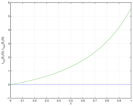
Figure 10: $\lambda_{min}[S_{\tau}(0)]$ and $\lambda_{max}[S_{\tau}(0)]$ versus $T$ with $\tau=1$.

From this plot, we can see that the matrix $S_{\tau}(0)$ is singular for all $T\in[0,1]$. Furthermore, we find that $S_{\tau}(0)x_{2}=0$ for all $T\in[0,1]$. Thus, using Theorem 4, it follows that with $\tau=1$, $W_{\tau}(x_{2},T)=\infty$ for all $T\in[0,1]$. Hence, it follows from Definition 5 that the state $x_{2}$ is not (differentially) possibly controllable.

We now apply the Kalman decomposition to this uncertain system; e.g., see [19, 20, 1]. Indeed, if we apply the state space transformation $\tilde{x}=Tx$ with $T=\left[\begin{array}[]{rr}-0.7435&0.6687\\ 0.6687&0.7435\end{array}\right]$ to this uncertain system, we obtain an uncertain system of the form (2), (2) defined by:

$$\tilde{A} = \left[\begin{array}[]{rr}-0.6000&0.0000\\ 1.0605&-0.9500\end{array}\right];~{}\tilde{B}_{1}=\left[\begin{array}[]{r}0.0000\\ 0.5848\end{array}\right];$$

$$\tilde{B}_{2} = \left[\begin{array}[]{r}0.0000\\ 1.0843\end{array}\right];~{}\tilde{C}_{1}=\left[\begin{array}[]{rr}-0.5465&0.3694\end{array}\right];$$

$$\tilde{D}_{1} = 0;~{}\tilde{C}_{2}=\left[\begin{array}[]{rr}0.8399&0.0082\end{array}\right];~{}\tilde{D}_{2}=0.$$

From this, the control input $u$ and the uncertainty input $\xi$ do not affect the first state of this system. Thus, we can remove this state without changing the input-output behavior of the system. This leads to a reduced dimension uncertain system described by the state equations

$$\dot{x} = -0.9500x+0.5848u+1.0843\xi;$$

$$z = 0.3694x;y=0.0082x$$

and the averaged IQC (2).

8.2 Example 2

This example considers an uncertain system corresponding to the electrical circuit shown in Figure 11.

\psfrag{u}{$u$}\psfrag{R1}{$R_{1}$}\psfrag{R2}{$R_{2}$}\psfrag{R3}{$R_{3}$}\psfrag{C1}{$C_{1}$}\psfrag{C2}{$C_{2}$}\psfrag{V1}{$V_{1}$}\psfrag{V2}{$V_{2}$}\psfrag{y}{$y$}\includegraphics[width=227.62204pt]{figure10.eps}

Figure 11: Electrical circuit corresponding to Example 2.

It is straightforward to derive the following state space model for this circuit:

$$\left[\begin{array}[]{c}\frac{dV_{1}}{dt}\\ \frac{dV_{2}}{dt}\end{array}\right] = \left[\begin{array}[]{cc}-\frac{1}{C_{1}}\left(\frac{1}{R_{3}}+\frac{1}{R_{1}}\right)&-\frac{1}{R_{3}C_{1}}\\ -\frac{1}{R_{3}C_{2}}&-\frac{1}{C_{2}}\left(\frac{1}{R_{3}}+\frac{1}{R_{2}}\right)\end{array}\right]\left[\begin{array}[]{c}V_{1}\\ V_{2}\end{array}\right]$$ (80)

$$+\left[\begin{array}[]{c}\frac{1}{C_{1}}\\ \frac{1}{C_{2}}\end{array}\right]u;$$

$$y = \left[\begin{array}[]{cc}0&1\end{array}\right]\left[\begin{array}[]{c}V_{1}\\ V_{2}\end{array}\right].$$ (84)

In this example, we choose the parameter values for the nominal to be $R_{1}=0.5\Omega$, $R_{2}=1.0\Omega$, $R_{3}=0.5\Omega$, $C_{1}=2.0F$, and $C_{2}=1.0F$. For these parameter values, the nominal system is not controllable.

We now consider two cases of uncertain parameters for this system. In the first case, we find that all non-zero states of the system are possibly controllable and no reduced dimension model can be constructed using the Kalman decomposition of Section 7. In the second case, we find that there exist non-zero states of the system which are not possibly controllable. Then, we use the Kalman decomposition of Section 7 to construct a model of order one which does not change the input-output behavior of the system.

Case 1. In this case, we suppose that the conductance of the resistor $R_{1}$ is uncertain and we write $\frac{1}{R_{1}}=2+\Delta$ where $|\Delta|\leq 1$. This leads to an uncertain system of the form (2) where

$$A = \left[\begin{array}[]{cc}-2&-1\\ -2&-3\end{array}\right];~{}~{}B_{1}=\left[\begin{array}[]{c}0.5\\ 1\end{array}\right];~{}~{}B_{2}=\left[\begin{array}[]{c}-0.5\\ 0\end{array}\right];$$

$$C_{1} = \left[\begin{array}[]{cc}1&0\end{array}\right];~{}~{}D_{1}=0;~{}~{}C_{2}=\left[\begin{array}[]{cc}0&1\end{array}\right];~{}~{}D_{2}=0;$$

and $\xi=\Delta z$. Since $|\Delta|\leq 1$, it follows that the averaged IQC (2) will be satisfied. For this uncertain system, we calculate the transfer functions $G(s)$ and $H(s)$ as

$$G(s) = \frac{1}{s^{2}+5s+4}\not\equiv 0;~{}~{}H(s)=\frac{0.5s+0.5}{s^{2}+5s+4}\not\equiv 0.$$

For this uncertain system, the pair $(A,B_{1})$ is not controllable. However, the pair $(A,[B_{1}~{}B_{2}])$ is controllable. Thus, it follows from Theorem 6 that the system has no states which are not differentially possibly controllable. Also, the pair $(\left[\begin{array}[]{l}C_{1}\\ C_{2}\end{array}\right],A)$ is observable and hence, using Case 4 of the Kalman decompositions considered in Section 7, we cannot construct an equivalent reduced dimension uncertain system corresponding to this uncertain system.

Note that the example considered in this case is such that the nominal system is not controllable, but the uncertain system becomes controllable for non-zero values of the uncertain parameter $\Delta$. If we change the parameter $C_{1}$ to $C_{1}=1$, we obtain an uncertain system for which the nominal system is controllable but for which the system becomes uncontrollable for one value of the uncertain parameter ($\Delta=-1$).

Case 2. In this case, we suppose that the conductance of the resistor $R_{3}$ is uncertain and we write $\frac{1}{R_{3}}=2+\Delta$ where $|\Delta|\leq 1$. This leads to an uncertain system of the form (2) where

$$A = \left[\begin{array}[]{cc}-2&-1\\ -2&-3\end{array}\right];~{}~{}B_{1}=\left[\begin{array}[]{c}0.5\\ 1\end{array}\right];~{}~{}B_{2}=\left[\begin{array}[]{c}-0.5\\ -1\end{array}\right];$$

$$C_{1} = \left[\begin{array}[]{cc}1&1\end{array}\right];~{}~{}D_{1}=0;~{}~{}C_{2}=\left[\begin{array}[]{cc}0&1\end{array}\right];~{}~{}D_{2}=0;$$

and $\xi=\Delta z$. For this uncertain system, we calculate the transfer functions $G(s)$ and $H(s)$ as

$$G(s) = \frac{-s-1}{s^{2}+5s+4}\not\equiv 0;~{}~{}H(s)=\frac{1.5s+1.5}{s^{2}+5s+4}\not\equiv 0.$$

For this uncertain system, the pair $(A,[B_{1}~{}B_{2}])$ is not controllable. Thus, it follows from Theorem 6 that the system has non-zero states which are not differentially possibly controllable. Also, the pair $(\left[\begin{array}[]{l}C_{1}\\ C_{2}\end{array}\right],A)$ is observable. We now construct the Kalman decomposition for this system as in Case 4 of Section 7. Indeed, we apply a state space transformation $\tilde{x}=Tx$ with $T=\left[\begin{array}[]{rr}-0.8944&0.4472\\ -0.4472&-0.8944\end{array}\right]$ to this uncertain system to obtain an uncertain system of the form (2), (2) defined by:

$$\tilde{A} = \left[\begin{array}[]{rr}-1.0000&0.0000\\ -1.0000&-4.0000\end{array}\right];~{}\tilde{B}_{1}=\left[\begin{array}[]{r}0.0000\\ -1.1180\end{array}\right];$$

$$\tilde{B}_{2} = \left[\begin{array}[]{r}-0.0000\\ 1.1180\end{array}\right];~{}\tilde{C}_{1}=\left[\begin{array}[]{rr}-0.4472&-1.3416\end{array}\right];$$

$$\tilde{D}_{1} = 0;~{}\tilde{C}_{2}=\left[\begin{array}[]{rr}0.4472&-0.8944\end{array}\right];~{}\tilde{D}_{2}=0.$$

From this, the control input $u$ and the uncertainty input $\xi$ do not affect the first state of this system. Thus, we can remove this state without changing the input-output behavior of the system. This leads to a reduced dimension uncertain system described by the state equations

$$\dot{x} = -4.0x-1.1180u+1.1180\xi;$$

$$z = -1.3416x;y=-0.8944x$$

and the averaged IQC (2).

9 Conclusions and Future Research

The results of this paper have led to a geometric characterization of the notion of possible controllability for a class of uncertain linear systems. These results combined with a corresponding geometric characterization of the notion of robust unobservability have allowed us to present a complete Kalman decomposition for uncertain systems.

Possible areas of future research motivated by the results of this paper include extending the results of the paper to the case of structured uncertainty subject to multiple IQCs.

References

- [1] P. J. Antsaklis and A. N. Michel, Linear Systems, 2nd ed. Boston: Birkhäuser, 2006.
- [2] I. R. Petersen, V. A. Ugrinovskii, and A. V. Savkin, Robust Control Design using Methods. Springer-Verlag London, 2000.
- [3] S. P. Bhattacharyya, “Generalized controllability, -invariant subspaces and parameter invariant control,” SIAM J. Algebraic Discrete Methods, vol. 4, no. 4, pp. 52–533, 1983.
- [4] I. R. Petersen, “Notions of stabilizability and controllability for a class of uncertain linear systems,” International Journal of Control, vol. 46, no. 2, pp. 409–422, 1987.
- [5] ——, “The matching condition and feedback controllability of uncertain linear systems,” in Robust Control of Linear Systems and Nonlinear Control, M. A. Kaashoek, J. H. van Schuppen, and A. C. M. Ran, Eds. Boston: Birkhäuser, 1990.
- [6] G. Conte, A. M. Perdon, and G. Marro, “Computing the maximum robust controlled invariant subspace,” Systems and Control Letters, vol. 17, no. 2, pp. 131–135, 1991.
- [7] G. Basile and G. Marro, Controlled and conditioned invariants in linear system theory. Englewood Cliffs, NJ: Prentice Hall, 1992.
- [8] A. V. Savkin and I. R. Petersen, “Weak robust controllability and observability of uncertain linear systems,” IEEE Transactions on Automatic Control, vol. 44, no. 5, pp. 1037–1041, 1999.
- [9] I. R. Petersen and A. V. Savkin, Robust Kalman Filtering for Signals and Systems with Large Uncertainties. Birkhäuser Boston, 1999.
- [10] I. R. Petersen, “Notions of observability for uncertain linear systems with structured uncertainty,” SIAM Journal on Control and Optimization, vol. 41, no. 2, pp. 345–361, 2002.
- [11] ——, “A notion of possible controllability for uncertain linear systems with structured uncertainty,” Automatica, vol. 45, no. 1, pp. 134–141, 2009.
- [12] ——, “Robust unobservability for uncertain linear systems with structured uncertainty,” IEEE Transactions on Automatic Control, vol. 52, no. 8, pp. 1461–1469, 2007.
- [13] ——, “A Kalman decomposition for robustly unobservable uncertain linear systems,” Systems and Control Letters, vol. 57, pp. 800–804, 2008.
- [14] C. L. Beck and J. C. Doyle, “A necessary and sufficient minimality condition for uncertain systems,” IEEE Transactions on Automatic Control, vol. 44, no. 10, pp. 1802–1813, 1999.
- [15] C. Beck and R. D’Andrea, “Noncommuting multidimensional realization theory: Minimality, reachability, and observability,” IEEE Transactions on Automatic Control, vol. 49, no. 10, pp. 1815–1820, 2004.
- [16] I. R. Petersen, “Equivalent realizations for uncertain systems with an IQC uncertainty description,” Automatica, vol. 43, no. 1, pp. 44–55, 2007.
- [17] W. S. Gray and J. P. Mesko, “Observability functions for linear and nonlinear systems,” Systems and Control Letters, vol. 38, pp. 99–113, 1999.
- [18] J. Scherpen and W. Gray, “Minimality and local state decompositions of a nonlinear state space realization using energy functions,” IEEE Transactions on Automatic Control, vol. 45, no. 11, pp. 2079–2086, 2000.
- [19] R. E. Kalman, “Mathematical descriptions of linear systems,” SIAM Journal on Control and Optimization, vol. 1, pp. 152–192, 1963.
- [20] ——, “On the computation of the reachable/observable canonical form,” SIAM Journal on Control and Optimization, vol. 20, no. 2, pp. 258–260, 1982.
- [21] A. V. Savkin and I. R. Petersen, “An uncertainty averaging approach to optimal guaranteed cost control of uncertain systems with structured uncertainty,” Automatica, vol. 31, no. 11, pp. 1649–1654, 1995.
- [22] ——, “Recursive state estimation for uncertain systems with an integral quadratic constraint,” IEEE Transactions on Automatic Control, vol. 40, no. 6, pp. 1080–1083, 1995.
- [23] D. J. Clements and B. D. O. Anderson, Singular Optimal Control: The Linear-Quadratic Problem. Berlin, Germany: Springer Verlag, 1978.