Multiple scattering theory of quasiparticles on a topological insulator surface

Abstract

A general partial-wave multiple scattering theory for scattering from cylindrically symmetric potentials on a topological insulator (TI) surface is developed. As an application, the cross sections for a single scatterer and two scatterers are discussed. We find that the symmetry of differential cross section is reduced and the backscattering is allowed for massive Dirac fermions on gapped TI surface. Remarkably, a sharp resonance peak at the band edge of the gapped TI is found in the total cross section $\Lambda_{tot}$, which may offer a useful way to determine the gap (as well as the effective mass of quasiparticles) on TI surface. We show that the interference effect is obvious in cross sections during the quasiparticle scattering between the scatterer pair, and additional resonance peaks are introduced in $\Lambda_{tot}$ when the higher partial waves are taken into account.

Topological insulator (TI) has attracted lots of interest in modern condensed matter physics field since the advanced progress in theoretical Kane ; Kane1 ; Bernevig ; Fu ; Fang and experimental Konig ; Hsieh1 ; Chen ; Xia studies of this new quantum matter phase. The ideal three-dimensional (3D) TI exhibits gapless modes on surface, and the backscattering is forbidden due to the time reversal invariance, which has been observed in the angle-resolved photo emission spectroscopy experiments on Bi₂Te₃ surface Hsieh2 . However, if the Dirac fermions gain mass, a gap will be induced in system, which breaks the time reversal symmetry Qi ; Hasan ; Maciejko and as a consequence, the scattering and transport properties should be different from the gapless case. Due to the single Dirac-cone nature, no complicated intervalley scattering events occur on TI surface. Therefore, it can be expected that in situ measurement or even manipulation of impurity scattering processes on TI surfaces should pave a promising way to study electronic structures and find extraordinary quantum phenomena in various TI materials. Recently, a series of scanning tunneling microscopy (STM) measurements Xue ; Roushan ; Gomes and theoretical simulations Liu ; Lee have been performed on Bi₂Te₃ and Bi_1-xSb_x surface states to study the scattering effect in the dilute impurity limit. On the other hand, when the impurities are located close to each other, the multiple scattering effects should be important. Especially, since the quasipartcle’s spin is strongly coupled to its momentum, then the quantum interference between different spin states during multiple scattering process may display profound phenomena such as electric conductance weak (anti-)localization He and Aharonov-Bohm effect Fu1 in STM signal. Therefore, it is clear that at present more deep multiple scattering studies are being called for.

In this work we conduct a multiple scattering theory for the massive as well as massless Dirac fermions on surfaces of 3D TIs. A general partial-wave multiple scattering formula for scattering from short-range cylindrically symmetric potentials is developed. The cross sections for a single scatterer and two scatterers are discussed, and the interference effect during the quasiparticle scattering between the scatterer pair is found. We show that higher partial waves induce prominent corrections in cross sections, including additional resonance peaks. The symmetry of differential cross section is reduced and the backscattering can be observed for massive Dirac fermions due to the breaking of the time reversal symmetry. Especially, a sharp resonance peak at the band edge of the gapped Dirac fermion is found in total cross section, which may offer a useful way to determine the gap of the TI surface states. Note that our formulation is closely related to those given on semiconductor heterostructure Walls1 and graphene Novikov ; Braun ; Walls . Remarkably, unlike graphene, the TI surface is a single Dirac-cone system, which makes the present intravalley multiple scattering theory more natural and exact.

We start from the effective-mass Hamiltonian near the Dirac point,

$$H_{0}=\hbar v_{F}\left(\boldsymbol{\sigma}\times\boldsymbol{k}\right)\cdot\hat{z}+\Delta\sigma_{3},$$ (1)

where $v_{F}\mathtt{\approx}5.0\mathtt{\times}10^{5}$m/s is the Fermi velocity, $\boldsymbol{\sigma}\mathtt{=}\left(\sigma_{1},\sigma_{2},\sigma_{3}\right)$ are Pauli matrices, $\boldsymbol{k}\mathtt{=}\left(k_{x},k_{y}\right)$ is the planer momentum, and $\Delta\mathtt{=}m^{\ast}v_{F}^{2}$ is the band-gap, which is absent in the massless limit. The eigenstates of $H_{0}$ are given by plane wave

$$\Psi_{0,\pm}\left(\boldsymbol{r}\right)=\frac{e^{i\boldsymbol{k}\cdot\boldsymbol{r}}}{\sqrt{2\left|\epsilon\right|}}\left(\begin{array}[c]{cc}\delta_{+},&\mp i\delta_{-}e^{i\theta_{\boldsymbol{k}}}\end{array}\right)^{T},$$ (2)

where $\delta_{\pm}\mathtt{=}\sqrt{\left|\epsilon\pm\Delta\right|},$ and $\epsilon\mathtt{=}\pm\sqrt{\left(\hbar v_{F}k\right)^{2}\mathtt{+}\Delta^{2}}$ with the upper (lower) sign referring to the electron (hole) part of the spectrum. The Berry phase of system given by $-i\int_{0}^{2\pi}d\theta_{k}\left\langle\Psi_{0,\pm}\right|\partial_{\theta_{k}}\left|\Psi_{0,\pm}\right\rangle\mathtt{=}\frac{\left|\epsilon-\Delta\right|}{\left|\epsilon\right|}\pi$ indicates that the backscattering is allowed (prohibited) if band-gap $\Delta\mathtt{\neq}0$ ($\mathtt{=}0$), which will be observed in differential cross section in the following discussion. To obtain the scattering theory from localized, cylindrically symmetric scatterers, it is convenient for boundary condition treatment to express the eigenstates for Eq. (1) in cylindrical coordinates, which are written as

$$\chi_{l,\pm}^{(1,2)}\left(\boldsymbol{r}\right)=\sqrt{\frac{k}{2\left|\epsilon\right|}}e^{il\theta}\left(\begin{array}[c]{cc}\delta_{+}H_{l}^{(1,2)},&\pm\delta_{-}H_{l+1}^{(1,2)}e^{i\theta}\end{array}\right)^{T},$$ (3)

for outgoing and incoming cylindrical waves about $\boldsymbol{r}$=$0$, respectively. Here $H_{l}^{(1,2)}$ are Hankel functions of order $l$ with variable $kr$.

The potential of each symmetric scalar scatterer can be expressed as

$$V\left(\boldsymbol{r}\right)=V_{0}\theta\left(a-r\right),$$ (4)

where $a$ is the radius of scatterer. The incident plane wave centered about a single scatterer located at $\boldsymbol{r}_{n}$ is given by

$$\Phi_{\pm}^{in}\left(\boldsymbol{r}\right)=\frac{e^{i\boldsymbol{k}\cdot\boldsymbol{r}_{n}}}{2\sqrt{k}}\sum_{l=-\infty}^{\infty}e^{il\left(\theta_{n}-\theta_{\boldsymbol{k}}\right)}i^{l}\left(\chi_{l,\pm}^{(1)}\left(\boldsymbol{\rho}_{n}\right)+\chi_{l,\pm}^{(2)}\left(\boldsymbol{\rho}_{n}\right)\right),$$ (5)

where $\chi_{l,\pm}^{(1)}$ and $\chi_{l,\pm}^{(2)}$ represent outgoing and incoming waves about $\boldsymbol{r}_{n}$, with $\boldsymbol{\rho}_{n}\mathtt{=}\boldsymbol{r}\mathtt{-}\boldsymbol{r}_{n}$ and $e^{i\theta_{n}}\mathtt{=}\frac{\boldsymbol{\rho}_{n}\cdot\left(\hat{x}+i\hat{y}\right)}{\rho_{n}}$. By using the boundary condition at $\rho_{n}\mathtt{=}a$, we can get the scattered wave function

$$\Psi_{\pm}^{sc}\left(\boldsymbol{r}\right)=s_{0}G_{+0}T_{0}^{-}\Phi_{\pm}^{in}+\sum_{l=1}^{\infty}\left[s_{l}G_{+l}T_{l}^{-}+s_{-l}G_{-l}T_{l}^{+}\right]\Phi_{\pm}^{in},$$ (6)

where the $l$th-partial wave $t\mathtt{-}$matrix is $T_{l}^{\pm}\mathtt{=}$diag$(\begin{array}[c]{cc}\hat{P}_{l}^{\pm},&\mp i\hat{P}_{l\mp 1}^{\pm}\end{array})$ with $\hat{P}_{l}^{\pm}\mathtt{=}\frac{1}{i^{l}k^{l}}(\partial_{x}\mathtt{\pm}i\partial_{y})^{l}\mathtt{=}\frac{e^{\pm il\theta}}{i^{l}k^{l}}(\partial_{r}\mathtt{\pm}\frac{i}{r}\partial_{\theta})^{l}$, and

$$G_{+l} =\frac{i^{l}e^{il\theta_{n}}}{2\left|\epsilon\right|}\left(\begin{array}[c]{cc}\delta_{+}^{2}H_{l}^{(1)}&\pm\delta_{+}\delta_{-}H_{l}^{(1)}\\ \pm\delta_{+}\delta_{-}H_{l+1}^{(1)}e^{i\theta_{n}}&\delta_{-}^{2}H_{l+1}^{(1)}e^{i\theta_{n}}\end{array}\right),$$ (9)

$$G_{-l} =\frac{i^{l}e^{-il\theta_{n}}}{2\left|\epsilon\right|}\left(\begin{array}[c]{cc}\delta_{+}^{2}H_{l}^{(1)}&\mp\delta_{+}\delta_{-}H_{l}^{(1)}\\ \mp\delta_{+}\delta_{-}H_{l-1}^{(1)}e^{i\theta_{n}}&\delta_{-}^{2}H_{l-1}^{(1)}e^{i\theta_{n}}\end{array}\right).$$ (12)

The variable of Hankel functions is $k\rho_{n}$. The scattering amplitude of the $l$th partial wave is

$$s_{l}=\frac{\tilde{A}^{+}J_{l}\left(ka\right)J_{l+1}\left(k^{\prime}a\right)-\tilde{A}^{-}J_{l+1}\left(ka\right)J_{l}\left(k^{\prime}a\right)}{\tilde{A}^{-}H_{l+1}^{(1)}\left(ka\right)J_{l}\left(k^{\prime}a\right)-\tilde{A}^{+}H_{l}^{(1)}\left(ka\right)J_{l+1}\left(k^{\prime}a\right)},$$ (13)

where $\tilde{A}^{\pm}\mathtt{=}\sqrt{\left|\frac{\epsilon\pm\Delta}{\epsilon-V_{0.}\pm\Delta}\right|}$, $k^{\prime}\mathtt{=}\sqrt{\left(\epsilon\mathtt{-}V_{0}\right)^{2}\mathtt{-}\Delta^{2}}/\hbar v_{F}$, and $J_{l}$ is the Bessel function of order $l$. In the massless limit, i.e., $\Delta\mathtt{=}0$, the above Eq. (6) can be reduced into a more compact form due to the symmetry of the band, which is written as

$$\Psi_{\pm}^{sc}\left(\boldsymbol{r}\right)=\sum_{l=0}^{\infty}\frac{4i\hbar v_{F}s_{l}}{k}G_{l}\left(\boldsymbol{r},\boldsymbol{r}_{n},\epsilon\right)T_{l}\left[\Phi_{\pm}^{in}\right],$$ (14)

where

$$G_{l}\propto\left(\begin{array}[c]{cc}H_{l}^{(1)}e^{il\theta_{n}}&\mp H_{l+1}^{(1)}e^{-i\left(l+1\right)\theta_{n}}\\ \pm H_{l+1}^{(1)}e^{i\left(l+1\right)\theta_{n}}&H_{l}^{(1)}e^{-il\theta_{n}}\end{array}\right),$$ (15)

and $T_{l}\mathtt{=}\mathtt{diag}(\begin{array}[c]{cc}\hat{P}_{l}^{-},&\hat{P}_{l}^{+}\end{array})$. Here, we have used the relation $s_{-(l+1)}\mathtt{=}s_{l}$ for $\Delta\mathtt{=}0$.

It is easy to extend the above theory to multiple scattering problems of massive quasiparticles on TI surface. The total wave function for $N$ scatterers located at positions $\boldsymbol{r}_{1},\boldsymbol{r}_{2},\cdots\boldsymbol{r}_{N}$ is given by $\Psi\left(\boldsymbol{r}\right)\mathtt{=}\Phi_{\pm}^{in}\mathtt{+}\Psi_{\pm}^{sc}$, where

$$\Psi_{\pm}^{sc}\left(\boldsymbol{r}\right)=\mathbb{G}\left(\boldsymbol{r}\right)\mathit{S}M^{-1}\vec{\phi}.$$ (16)

Here, $\mathbb{G}\left(\boldsymbol{r}\right)$ is a $2\mathtt{\times}2N\left(2l_{\max}\mathtt{+}1\right)$ matrix,

$$\mathbb{G}\left(\boldsymbol{r}\right)=\left(\begin{array}[c]{ccc}\tilde{G}\left(\boldsymbol{r},\boldsymbol{r}_{1}\right),&\tilde{G}\left(\boldsymbol{r},\boldsymbol{r}_{2}\right),&\cdots,\end{array}\begin{array}[c]{c}\tilde{G}\left(\boldsymbol{r},\boldsymbol{r}_{N}\right)\end{array}\right)$$ (17)

with $\tilde{G}\mathtt{=}[\begin{array}[c]{ccc}G_{+0},&G_{+1},&G_{-1},\end{array}\cdots,\begin{array}[c]{cc}G_{+l_{\max}},&G_{-l_{\max}}\end{array}]$. $\mathit{S}$ is a $2N\left(2l_{\max}\mathtt{+}1\right)\mathtt{\times}2N\left(2l_{\max}\mathtt{+}1\right)$ diagonal matrix with the nontrivial elements $s_{0}$ and $s_{\pm l}$. $M$ is expressed by

$$M=\mathbf{1}-\mathbf{G}\mathit{S},$$ (18)

where

$$\mathbf{G=}\text{$\left(\begin{array}[c]{cccc}\mathbf{0}&\mathbf{G}\left(1,2\right)&\mathbf{\cdots}&\mathbf{G}\left(1,N\right)\\ \mathbf{G}\left(2,1\right)&\mathbf{0}&\mathbf{\cdots}&\mathbf{G}\left(2,N\right)\\ \mathbf{\vdots}&\mathbf{\vdots}&\mathbf{\ddots}&\vdots\\ \mathbf{G}\left(N,1\right)&\mathbf{G}\left(N,2\right)&\cdots&\mathbf{0}\end{array}\right),$}$$ (19)

with $\mathbf{G}\left(i,j\right)$ are $2\left(2l_{\max}\mathtt{+}1\right)\mathtt{\times}2\left(2l_{\max}\mathtt{+}1\right)$ matrices constructed by $T_{l}^{\pm}\left[G_{l^{\prime}}^{k}\left(i,j\right)\right]$ ($0\mathtt{\leq}l,l^{\prime}\mathtt{\leq}l_{\max}$). Finally, $\vec{\phi}$ can be written as a $2N\left(2l_{\max}\mathtt{+}1\right)\mathtt{\times}1$ vector, explicitly,

$$\vec{\phi}=\left(\begin{array}[c]{cccc}\phi_{1},&\phi_{2},&\cdots,&\phi_{N}\end{array}\right)^{T},$$ (20)

where $\phi_{i}\mathtt{=}\left[\begin{array}[c]{cccc}T_{0}^{-}\left[\Phi\left(\boldsymbol{r}_{i}\right)\right],&T_{1}^{-}\left[\Phi\left(\boldsymbol{r}_{i}\right)\right],&T_{1}^{+}\left[\Phi\left(\boldsymbol{r}_{i}\right)\right],&\mathtt{\cdots},\end{array}\right.\left.\begin{array}[c]{cc}T_{l_{\max}}^{-}\left[\Phi\left(\boldsymbol{r}_{i}\right)\right],&T_{l_{\max}}^{+}\left[\Phi\left(\boldsymbol{r}_{i}\right)\right]\end{array}\right]^{T}$. The multiple scattering problem will be simplified in the massless limit $\Delta\mathtt{=}0$, and similar to the case of a single scatterer, some transformations, including $s_{-(l+1)}\mathtt{=}s_{l}$, $(T_{l}^{+},T_{l}^{-})\mathtt{\rightarrow}T_{l}$, and $(G_{+l},G_{-l})\mathtt{\rightarrow}G_{l}$, should be performed in Eqs. (16-20). Consequently, matrices $M$ and $\mathit{S}$ are reduced to $2N\left(l_{\max}\mathtt{+}1\right)\mathtt{\times}2N\left(l_{\max}\mathtt{+}1\right)$ ones, which are similar to the problems of intravalley multiple scattering of quasiparticles in graphene Walls , so that we do not show the explicit formulas for the case of $\Delta\mathtt{=}0$ herein.

The above theory allows one to solve the multiple scattering problems on gapped or gapless TI surface with higher partial waves, which may be important as the distance between scatterers decreases as well as the scattering potential is strong. If the potential is very weak, $s\mathtt{-}$wave ($l_{\max}$=$0$) is enough. To obtain the scattering amplitude and the cross section, we apply the following approximation on Hankel functions $H_{l}^{\left(1\right)}$ in Eq. (17) for $r\mathtt{\rightarrow}\infty$,

$$H_{l}^{\left(1\right)}\left(k\rho_{n}\right)\rightarrow\sqrt{\frac{2}{i^{2l+1}\pi kr}}e^{ikr}e^{-ik\hat{r}\cdot\boldsymbol{r}_{n}},$$ (21)

and $e^{i\theta_{n}}\mathtt{=}\boldsymbol{\rho}_{n}\mathtt{\cdot}\left(\hat{x}\mathtt{+}i\hat{y}\right)/\rho_{n}\mathtt{\rightarrow}\hat{r}\mathtt{\cdot}\left(\hat{x}\mathtt{+}i\hat{y}\right)\mathtt{=}e^{i\varphi}$, where $\hat{r}\mathtt{=}\left(\cos\varphi\mathtt{,}\sin\varphi\right)$ is a unit vector in the direction of $\boldsymbol{r}$. Finally, the scattered wave function can be approximated as

$$\Psi_{\pm}^{sc}\left(\boldsymbol{r}\right)\rightarrow f\left(\boldsymbol{k},\varphi\right)\frac{1}{\sqrt{2\left|\epsilon\right|}}\left(\begin{array}[c]{cc}\delta_{+},&\mp i\delta_{-}e^{i\varphi}\end{array}\right)^{T}\frac{e^{ikr}}{\sqrt{r}},$$ (22)

where $f\left(\boldsymbol{k},\varphi\right)$ is nothing else but the scattering amplitude. Therefore, the differential cross section should be

$$d\Lambda/d\varphi=\left|f\left(\boldsymbol{k},\varphi\right)\right|^{2},$$ (23)

and the total cross section is

$$\Lambda_{tot}=\int_{0}^{2\pi}d\varphi\left|f\left(\boldsymbol{k},\varphi\right)\right|^{2}=C_{\Delta}\sqrt{\frac{8\pi}{k}}\operatorname{Im}\left[e^{-i\frac{\pi}{4}}f\left(\boldsymbol{k},\varphi=0\right)\right],$$ (24)

The second equality for $\Lambda_{tot}$ expresses the 2D optical theorem in terms of our definition of $f$. $C_{\Delta}\mathtt{=}\left(\delta_{+}^{2}\mathtt{+}\delta_{-}^{2}\right)/2\left|\epsilon\right|$ arises from the band gap, which reduces to unity in the massless limit. On the other hand, the scattered current $\boldsymbol{j}_{sc}\mathtt{=}\mathtt{\mp}v_{F}\frac{\delta_{+}\delta_{-}}{\left|\epsilon\right|}\frac{\left|f\left(\boldsymbol{k},\varphi\right)\right|^{2}}{r}\left[\cos\varphi\hat{x}\mathtt{+}\sin\varphi\hat{y}\right]$, and the incident current $\boldsymbol{j}_{in}\mathtt{=}\mathtt{\mp}v_{F}\frac{\delta_{+}\delta_{-}}{\left|\epsilon\right|}\left[\cos\theta_{k}\hat{x}\mathtt{+}\sin\theta_{k}\hat{y}\right]$, which result in $d\Lambda/d\varphi\mathtt{=}r\left|\boldsymbol{j}_{sc}\right|/\left|\boldsymbol{j}_{in}\right|\mathtt{=}\left|f\left(\boldsymbol{k},\varphi\right)\right|^{2}$. In the following calculations, without losing generality, we just consider the incident wave $\Phi_{+}^{in}\mathtt{=}\frac{e^{ikx}}{\sqrt{2\left|\epsilon\right|}}(\begin{array}[c]{cc}\delta_{+}\mathtt{,}&\mathtt{-}i\delta_{-}\end{array})^{T}$ propagating along the positive $\hat{x}$ direction.

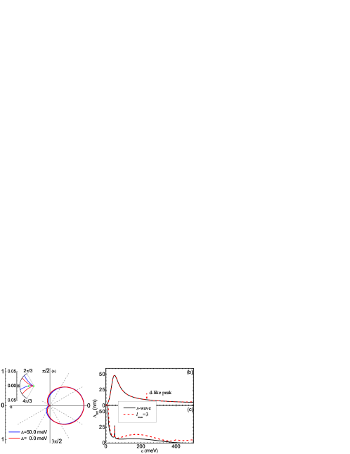
Figure 1: (Color online) The normalized differential (a) and the total (b-c) cross sections for a single scatterer. In (a), the red (blue) curve is for $\Delta\mathtt{=}0$ meV ($\Delta\mathtt{=}50$ meV), and $\epsilon\mathtt{=}320$ meV. (b) is for $\Delta\mathtt{=}0$ meV, while (c) is for $\Delta\mathtt{=}50$ meV. Insert in (a) is a zoom of $d\Lambda/d\varphi$ in angle range $[2\pi/3,4\pi/3]$, and the green dots indicate that the backscattering is allowed (forbidden) in the case of $\Delta\mathtt{\neq}0$ ($\Delta\mathtt{=}0$). In all calculations, $V_{0}\mathtt{=}2$ eV, and $a\mathtt{=}1$ nm are chosen.

Firstly, we discuss the single nonmagnetic scatterer problem. The numerical results of scattering cross section are shown in Fig. 1. From Fig. 1(a), one can observe that the backscattering at potential is absent when the band gap decreases to zero, i.e., the differential cross section $\left.d\Lambda\left(\Delta\mathtt{=}0\right)/d\varphi\right|_{\varphi=\pi}\mathtt{=}0$ [see the red curve in Fig. 1(a)]. This is also can be seen from the $l$th$\mathtt{-}$partial wave scattering amplitude

$$f_{l}^{\Delta=0}=2\sqrt{\frac{2}{i\pi k}}s_{l}\cos\left[\left(2l+1\right)\varphi/2\right]e^{-i\varphi/2},$$ (25)

which results in $f_{l}^{\Delta=0}\left(\varphi\mathtt{=}\pi\right)\mathtt{=}0$. However, on the band-gapped TI surface, the $l$th partial wave scattering amplitude becomes

$$f_{\pm l}^{\Delta\neq 0}=C_{\Delta}\sqrt{\frac{2}{i\pi k}}s_{\pm l}e^{\pm il\varphi},$$ (26)

which indicates $\left.d\Lambda\left(\Delta\mathtt{\neq}0\right)/d\varphi\right|_{\varphi=\pi}\mathtt{=}\left|\sum_{l=0}^{l_{\max}}f_{\pm l}^{\Delta\neq 0}\left(\varphi\mathtt{=}\pi\right)\right|^{2}\mathtt{\neq}0$ since the time-reversal symmetry is broken by the nonzero gap in the surface Dirac spectrum. The blue curve in Fig. 1(a) is for $d\Lambda/d\varphi$ corresponding to $\Delta\mathtt{=}50$ meV. It is clear that the symmetry of $d\Lambda\left(\Delta\mathtt{\neq}0\right)/d\varphi$ is reduced and the backscattering is allowed. This can be more clearly seen from the insert in 1(a), which enlarges $d\Lambda/d\varphi$ in angle range $\left[2\pi/3,4\pi/3\right]$.

The total cross section $\Lambda_{tot}$ as a function of energy $\epsilon$ is shown in Fig. 1(b) and 1(c) for the gapless and gapped TI surface. On average, the contributions from higher partial waves are much smaller than $s\mathtt{-}$wave ($\left|f_{0}\right|\mathtt{\gg}\left|f_{l\neq 0}\right|$) in low-energy scattering regime, see the black curves in Fig. 1(b) and 1(c) which only takes into account the $s\mathtt{-}$wave in calculations. However, we find that higher partial waves may introduce some remarkable corrections. For example, we find an additional resonance peak ($d\mathtt{-}$like peak) around $\epsilon\mathtt{=}233$ meV when the $f_{l=2}^{\Delta=0}$ partial wave is taken into account, while much higher partial wave has little corrections on $\Lambda_{tot}$, see the red dashed curves in Fig. 1(b). This additional peak arises from the pole of $\left|s_{l=2}\right|$, which could be obtained by expanding $\left|s_{l=2}\right|$ at this point. The pole of $\left|s_{l=1}\right|$ is out of the energy range we considered here, therefore, the corrections from $p\mathtt{-}$wave is small in Fig. 1(b). Furthermore, we can find that $\Lambda_{tot}$ for $\Delta\mathtt{\neq}0$ [Fig. 1(c)] is totally different from that for $\Delta\mathtt{=}0$. A sharp peak at the band edge $\epsilon$=$\Delta$ is found. In fact, $\epsilon$=$\Delta$ is a pole of $\left|s_{l}\right|$ for arbitrary $l$th partial wave. Therefore, we can conclude that this sharp peak in $\Lambda_{tot}$, which can be easily measured in scattering experiment, may provide a useful way to determine the band gap (as well as the effective mass $m^{\ast}$ of quasiparticle) of TI surface. The contributions from higher partial waves are obvious when $\epsilon\mathtt{>}\Delta$ [the red dashed curve in Fig. 1(c)].

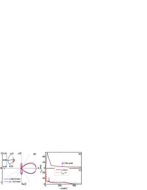
Figure 2: (Color online) The same as in Fig. 1 for two identical scatterers separated by distance $d\mathtt{=}6$ nm on a TI surface. $\boldsymbol{r}_{1}\mathtt{=}(-3,0)$ and $\boldsymbol{r}_{2}\mathtt{=}(3,0)$. Other parameters are chosen as the same as in Fig. 1.

Now let us discuss the double-scatterer case. The analytical expressions of the scattering amplitude for multiple scatterers are complicated, especially when taking into account the higher partial waves and the band gap. In the limit of $\Delta\mathtt{=}0$, the differential cross section for two identical scatterers located at $\boldsymbol{r}_{1/2}\mathtt{=}\left(\pm d/2,0\right)$ becomes symmetric since $M$ is symmetric. For instance, if we just consider the $s\mathtt{-}$wave, we can obtain the scattering amplitude

$$f_{0}^{\Delta=0} =\sqrt{\frac{2}{i\pi k}}s_{0}\sum_{n,m=1}^{2}e^{i\left(\boldsymbol{k}\cdot\boldsymbol{r}_{m}-k\hat{r}\cdot\boldsymbol{r}_{n}\right)}$$

$$\times\left\{\left[M_{0}^{-1}\right]_{2n-1,2m-1}\pm i\left[M_{0}^{-1}\right]_{2n,2m-1}e^{-i\varphi}\right.$$

$$\left.\mp i\left[M_{0}^{-1}\right]_{2n-1,2m}+\left[M_{0}^{-1}\right]_{2n,2m}e^{-i\varphi}\right\},$$ (27)

where

$$M_{0}^{-1}=\frac{1}{D}\text{$\left(\begin{array}[c]{cccc}1&0&s_{0}H_{0}&\pm s_{0}H_{1}\\ 0&1&\mp s_{0}H_{1}&s_{0}H_{0}\\ s_{0}H_{0}&\mp s_{0}H_{1}&1&0\\ \pm s_{0}H_{1}&s_{0}H_{0}&0&1\end{array}\right)$}$$ (28)

with $D\mathtt{=}\sqrt{\det\left|M_{0}\right|}\mathtt{=}1\mathtt{-}s_{0}^{2}\{[H_{0}^{\left(1\right)}\left(kd\right)]^{2}\mathtt{+}[H_{1}^{\left(1\right)}\left(kd\right)]^{2}\}$. It is easy to find that $f_{0}\left(\boldsymbol{k},\pi\right)\mathtt{=}0$, which indicates that the backscattering is also prohibited. This property can be clearly seen from the red curve in Fig. 2(a) as well as the inset of Fig. 2(a). However, the symmetry is reduced by the nonzero gap and the backscattering can occur, see the blue curve in Fig. 2(a). Besides, we find that the scattering along the directions of $\varphi\mathtt{\sim}60^{\circ}$, $120^{\circ}$, $240^{\circ}$, and $300^{\circ}$ is forbidden since the interference effect along these directions is destructive during the multiple scattering process. In the forward direction ($\varphi\mathtt{=}0$), however, the interference is still constructive. Moreover, comparing to the single-scatterer case, the width of resonance peak is narrowed and the peak is pushed to lower energy due to the interference during quasiparticle scattering between the impurity pair. Also, the higher partial waves introduce additional resonance peaks in $\Lambda_{tot}$, see the red curve in Fig. 2(b) and 2(c).

In principle, one can get the cross section as well as other transport properties for $N\mathtt{\ }$scatterers on the TI surface by the above theory. Before ending this paper, we calculated $\Lambda_{tot}$ for three scatterers to demonstrate the optical theorem in Eq. (24). For simplicity, we set $\Delta\mathtt{=}0$ and $l_{\max}\mathtt{=}3$ in calculations, and the results are shown in Fig. 3, in which the black curve is obtained by numerical integral while the red dashed curve is obtained from the second equality in Eq. (24). We can see that they are in good agreement with each other. Therefore we believe the optical theorem in Eq. (24) should be proper to characterize the general multiple scattering process.

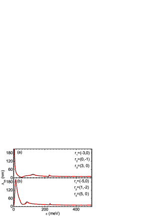
Figure 3: (Color online) Optical theorem Eq. (24) for three scatterers. The black (red dashed) curves are results in the first (second) equality in Eq. (24). $\Delta\mathtt{=}0$ and $l_{\max}\mathtt{=}5$ are chosen in calculations.

In summary, we have developed a general partial-wave multiple scattering theory for scattering from cylindrically symmetric potentials on TI surfaces and applied to cross section calculations. We have found that higher partial waves may introduce some important corrections in low-energy scattering. Importantly, a resonance peak at the band edge of the gapped TI surface was found, which should be easily measured in scattering experiments. This prediction may provide a useful way to determine the band gap of TI surface states. Our formulation can be extended to magnetic impurity scattering as well as spin-orbit coupled scattering on TI surface.

This work was supported by NSFC under Grants No. 90921003, No. 60776063, No. 60821061, and 60776061, and by the National Basic Research Program of China (973 Program) under Grants No. 2009CB929103 and No. G2009CB929300.

References

• (1) C. L. Kane and E. J. Mele, Phys. Rev. Lett. 95, 226801 (2005).
• (2) C. L. Kane and E. J. Mele, Phys. Rev. Lett. 95, 146802 (2005).
• (3) B. A. Bernevig, T. L. Hughes, and S.-C. Zhang, Science 314, 1757 (2006).
• (4) L. Fu, C. L. Kane, and E. J. Mele, Phys. Rev. Lett. 98, 106803 (2007); L. Fu and C. L. Kane, Phys. Rev. B 76, 045302 (2007).
• (5) H. J. Zhang, C. X. Liu, X. L. Qi, X. Dai, Z. Fang, and S. C. Zhang, Nat. Phys. 5, 438 (2009).
• (6) M. König et al., Science 318, 766 (2007).
• (7) D. Hsieh et al., Nature 452, 970 (2008); D. Hsieh et al., Phys. Rev. Lett. 103, 146401 (2009).
• (8) Y. L. Chen et al., Science 325, 178 (2009).
• (9) Y. Xia et al., Nat. Phys. 5, 398 (2009).
• (10) D. Hsieh et al., Science 323, 919 (2009).
• (11) X.-L. Qi, T. L. Hughes, and S.-C. Zhang, Phys. Rev. B 78, 195424 (2008).
• (12) M. Z. Hasan and C. L. Kane, Rev. Mod. Phys. 82, 3045 (2010).
• (13) J. Maciejko, X.-L. Qi, H. D. Drew, and S.-C. Zhang, Phys. Rev. lett. 105, 166803 (2010).
• (14) T. Zhang, et al., Phys. Rev. Leet. 130, 266803 (2009).
• (15) P. Roushan, et al., Nature 460, 1106 (2009).
• (16) K. K. Gomes, et al., arXiv:0909.0921 (2009).
• (17) Q. Liu, C.-X. Liu, C. Xu, X.-L. Qi, and S.-C. Zhang, Phys. Rev. Lett. 102, 156603 (2009).
• (18) W.-C. Lee, C. Wu, D. P. Arovas, and S.-C. Zhang, 80, 245439 (2009).
• (19) H.-T. He, et al., Phys. Rev. Lett. 106, 166805 (2011).
• (20) Z.-G. Fu, P. Zhang, and S.-S. Li, arXiv:1103.1710v1 (2011).
• (21) J. D. Walls, J. Huang, R. M. Westervelt, and E. J. Heller, Phys. Rev. B 73, 035325 (2006).
• (22) D. S. Novikov, Appl. Phys. Lett. 91, 102102 (2007); Phys. Rev. B 76, 245435 (2007).
• (23) M. Braun, L. Chirolli, and G. Burkard, Phys. Rev. B 77, 115433 (2008).
• (24) J. Y. Vaishnav, J. Q. Anderson, and Jamie D. Walls, Phys. Rev. B 83, 165437 (2011).