Upper bound on the rate of adaptation in an asexual population

Abstract

We consider a model of asexually reproducing individuals. The birth and death rates of the individuals are affected by a fitness parameter. The rate of mutations that cause the fitnesses to change is proportional to the population size, $N$. The mutations may be either beneficial or deleterious. In a paper by Yu, Etheridge and Cuthbertson [Ann. Appl. Probab. 20 (2010) 978–1004] it was shown that the average rate at which the mean fitness increases in this model is bounded below by $\log^{1-\delta}N$ for any $\delta>0$. We achieve an upper bound on the average rate at which the mean fitness increases of $O(\log N/(\log\log N)^{2})$.

t1Supported in part by NSF Grant DMS-08-05472.

1 Introduction

In a finite, asexually reproducing population with mutations, it is well known that competition among multiple individuals that get beneficial mutations can slow the rate of adaptation. This phenomenon is known as the Hill–Robertson effect, named for the authors of HR . One may wish to consider the effect on the rate of adaptation of a population when there are many beneficial mutations present simultaneously. It is easily observed that when such a population is finite and all mutations are either neutral or deleterious, the fitness of the population will decrease over time. This scenario is known as Muller’s ratchet. The first rigorous results regarding Muller’s ratchet were due to Haigh H . In an asexually reproducing population, beneficial mutations are necessary to overcome Muller’s ratchet. Yu, Etheridge and Cuthbertson YEC proposed a model that gives insight into both the Hill–Robertson effect and Muller’s ratchet in large populations with fast mutation rates.

The model introduced in YEC is a Moran model with mutations and selection. There are $N$ individuals in this model, each with an integer valued fitness. The dynamics of the model are determined by three parameters, $\mu$, $q$ and $\gamma$, which are independent of $N$. The parameters must satisfy $\mu>0$, $0<q\leq 1$ and $\gamma>0$. Let $X_{t}^{i}$ be the fitness of individual $i$ at time $t$. Then $X=(X^{1},X^{2},\ldots,X^{N})$ is a stochastic process with state space $\mathbb{Z}^{N}$. The system has the following dynamics: [(3)]

Mutation: Each individual acquires mutations at rate $\mu$. When individual $i$ gets a mutation, it is beneficial with probability $q$ and $X^{i}$ increases by 1. With probability $1-q$ the mutation is deleterious and $X^{i}$ decreases by 1.

Selection: For each pair of individuals $(i,j)$, at rate $\frac{\gamma}{N}(X^{i}-X^{j})^{+}$, we set $X^{j}$ equal to $X^{i}$.

Resampling: For each pair of individuals $(i,j)$, at rate $1/N$, we set $X^{j}$ equal to $X^{i}$. Note that the upper bound we establish for the rate of adaptation still holds in the absence of deleterious mutations, which corresponds to the case $q=1$. Under the selection mechanism the event that $X^{j}$ is set to equal $X^{i}$ represents the more fit individual $i$ giving birth and the less fit individual $j$ dying. Likewise, the resampling event that causes $X^{j}$ to equal $X^{i}$ represents individual $i$ giving birth and individual $j$ dying.

We give an equivalent description of the model involving Poisson processes that may make the coupling arguments more clear. The Poisson processes that determine the dynamics of $X$ are as follows:

• There are $N$ Poisson processes $\mathcal{P}^{i\uparrow}$, $1\leq i\leq N$, on $[0,\infty)$ of rate $q\mu$. If $\mathcal{P}^{i\uparrow}$ gets a mark at $t$ then the $i$th coordinate of $X$ increases by 1 at time $t$.

• There are $N$ Poisson processes $\mathcal{P}^{i\downarrow}$, $1\leq i\leq N$, on $[0,\infty)$ of rate $(1-q)\mu$. If $\mathcal{P}^{i\downarrow}$ gets a mark at $t$ then the $i$th coordinate of $X$ decreases by 1 at time $t$.

• For each ordered pair of coordinates $(i,j)$ with $i\neq j$ there is a Poisson process on $[0,\infty)$, $\mathcal{P}^{i,j}$, of rate $1/N$. If $\mathcal{P}^{i,j}$ gets a mark at $t$ then the $j$th coordinate changes its value to agree with the $i$th coordinate at time $t$.

• For each ordered pair of coordinates $(i,j)$ with $i\neq j$ there is a Poisson processes on $[0,\infty)\times[0,\infty)$, $\mathcal{P}^{i,j\uparrow}$, which has intensity $\frac{\gamma}{N}\lambda$ where $\lambda$ is Lebesgue measure on $\mathbb{R}^{2}$. If $\mathcal{P}^{i,j\uparrow}$ gets a mark in $\{t\}\times[0,X_{t-}^{i}-X_{t-}^{j}]$ then the $j$th coordinate changes its value to agree with the $i$th coordinate at time $t$.

A heuristic argument in YEC shows that as $N$ tends to infinity the mean rate of increase of the average fitness of the individuals in $X$ is $O(\log N/\break(\log\log N)^{2})$. Due to a typo on page 989 they state that the rate is $O(\log N/\break\log\log N)$. By equation (10) in YEC ,

$$K\log(\gamma K)=2\log N.$$

This implies that

$$K\approx\frac{2\log N}{\log\log N}.$$

Plugging $2\log N/\log\log N$ into each side of the consistency condition that they derive gives a rate of adaption of $O(\log N/(\log\log N)^{2})$.

The heuristic argument is difficult to extend to a rigorous argument. Let

$$\overline{X}=\frac{1}{N}\sum_{i=1}^{N}X^{i}$$

be the continuous-time process which represents the average fitness of the individuals in $X$. The rigorous results established in YEC are as follows:

• The centered process $X^{C}$, in which individual $i$ has fitness $X^{C,i}=X^{i}-\overline{X}$, is ergodic and has a stationary distribution $\pi$.

• If

  $$c_{2}=\frac{1}{N}\sum_{i=1}^{N}\bigl{(}X^{C,i}\bigr{)}^{2}$$

  is the variance of the centered process under the stationary distribution, then

  $$E^{\pi}[\overline{X}_{t}]=\bigl{(}\mu(2q-1)+\gamma E^{\pi}[c_{2}]\bigr{)}t,$$

  where $E^{\pi}$ means that the initial configuration of $X$ is chosen according to the stationary distribution $\pi$.

• For any $\delta>0$ there exists $N_{0}$ large enough so that for all $N\geq N_{0}$ we have $E\pi[\overline{X}_{1}]\geq\log^{1-\delta}N$.

It is difficult to say anything rigorous about $E^{\pi}[c_{2}]$ so other methods are needed to compute $E[\overline{X}_{t}]$. The third result of YEC shows that if there is a positive ratio of beneficial mutations then a large enough population will increase in fitness over time. A paper by Etheridge and Yu EY provides further results pertaining to this model.

Other similar models can be found in the biological literature. In these models the density of the particles is assumed to act as a traveling wave in time. The bulk of the wave behaves approximately deterministically and the random noise comes from the most fit classes of individuals. One tries to determine how quickly the fittest classes advance and pull the wave forward. This traveling wave approach is used in YE and YEC to approximate the rate of evolution as $O(\log N/(\log\log N)^{2})$. For other work in this direction see Rouzine, Brunet and Wilke RBW , Brunet, Rouzine and Wilke BRW , Desai and Fisher DF and Park, Simon and Krug PSK . Using nonrigorous arguments, these authors get estimates of $O(\log N)$, $O(\log N/\log\log N)$ and $O(\log N/(\log\log N)^{2})$, where the differences depend on the details of the models that they analyze. For more motivation and details concerning this model, please see the Introduction in YEC .

Motivated by applications to cancer development, Durrett and Mayberry have established rigorous results for a similar model in DM . They consider two models in which all mutations are beneficial and the mutation rate tends to 0 as the population size tends to infinity. In one of their models the population size is fixed and in the other it is exponentially increasing. For the model with the fixed population size they show that the rate at which the average fitness is expected to increase is $O(\log N)$. By considering the expected number of individuals that have fitness $k$ at time $t$, they establish rigorously that the density of the particles in their model will act as a traveling wave in time.

Our result is the following theorem.

Theorem 1

Let $X_{0}^{i}=0$ for $1\leq i\leq N$. There exists a positive constant $C$ which may depend on $\mu$, $q$ and $\gamma$ such that for $N$ large enough

$$\frac{E[\overline{X}]}{t}\leq\frac{C\log N}{(\log\log N)^{2}}$$

for all $t\geq\log\log N$.

A difference between the result in YEC and our result is that in YEC the initial state of the process is randomly chosen according to the stationary distribution $\pi$, while we make the assumption that all of the individuals initially have fitness 0.

The statements of the propositions needed to prove Theorem 1 and the proof of Theorem 1 are included in Section 2. At the end of the paper there is a table which includes the notation that is used throughout the paper and the Appendix that includes some general results on branching processes.

2 Proof of Theorem 1

Before stating the propositions we use to prove the theorem we need to establish some notation. Let $X_{t}^{+}=\max\{X_{t}^{i}\dvtx 1\leq i\leq N\}$ be the maximum fitness of any individual at time $t$ and $X_{t}^{-}=\min\{X_{t}^{i}\dvtx 1\leq i\leq N\}$ be the minimum fitness of any individual at time $t$. Define the width of the process to be $W_{t}=X_{t}^{+}-X_{t}^{-}$ and define $D_{t}=X_{t}^{+}-X_{0}^{+}$ be the distance the front of the process has traveled by time $t$. Theorem 1 states that all individuals initially have fitness 0. Therefore, a bound on $D_{t}$ immediately yields a bound on $\overline{X}_{t}$. The bounds we establish on $D_{t}$ will depend on the width, $W_{t}$.

Let $w=w(N)$ be any positive, increasing function that satisfies

$$\lim_{N\rightarrow\infty}w(N)=\infty\quad\mbox{and}\quad\lim_{N\rightarrow\infty}\frac{w(N)}{\log\log N}=0.$$

Let $\mathcal{W}=\lfloor w\log N/\log\log N\rfloor$ and $\mathcal{T}=w^{-1/2}\log\log N$. Heuristically, we conjecture that $W_{t}$ is typically of size $O(\log N/\log\log N)$ so $\mathcal{W}$ is larger than the typical width of $X$. With probability tending to 1, selection should cause any width larger than $\mathcal{W}$ to shrink within $\mathcal{T}$ time units. Because the width is a stochastic process, we are motivated to make the following definitions:

$$t_{1} = 0,$$

$$s_{n} = \inf\{t\geq t_{n}\dvtx W_{t}\geq 2\mathcal{W}\}\qquad\mbox{for }n\geq 1,$$

$$t_{n} = \inf\{t\geq s_{n-1}\dvtx W_{t}<\mathcal{W}\}\qquad\mbox{for }n\geq 2,$$

$$Y_{i} = \sup_{s_{i}\leq t\leq t_{i+1}}D_{t}-D_{s_{i}}\qquad\mbox{for }i\geq 1,$$

$$N_{t} = \max\{i\dvtx s_{i}\leq t\}\qquad\mbox{for }t\geq 0.$$

Note that $s_{n}$ and $t_{n}$ exist for all $n\geq 1$ with probability 1.

We define branching processes $Z^{k,\uparrow}$ for $k\geq 0$ which have the following dynamics:

• Initially there are $N$ particles of type $k$ in $Z_{0}^{k,\uparrow}$.

• Each particle changes from type $i$ to $i+1$ at rate $\mu$.

• A particle of type $i$ branches at rate $\gamma i+1$ and, upon branching, the new particle is also type $i$.

Let $\overline{M}{}^{k,\uparrow}_{t}$ be the maximum type of any particle in $Z_{t}^{k,\uparrow}$ and let $M_{t}^{k,\uparrow}=\overline{M}{}^{k,\uparrow}_{t}-k$, so that $M_{0}^{k,\uparrow}=0$. Note that we refer to individuals in branching processes as particles to distinguish them from the individuals in $X$. This will make the coupling arguments in the next section more clear.

We define a stochastic process $X^{\prime}$ that will be coupled with $X$ as described in the proof of Proposition 2 for reasons that will become clear shortly. Let $\{\mathcal{Z}^{n}\}_{n=0}^{\infty}$ be an i.i.d. sequence of continuous-time stochastic processes which each have the same distribution as $Z^{\mathcal{W},\uparrow}$. Let $\overline{\mathcal{M}}{}^{n}_{t}$ be the maximum type of any particle in $\mathcal{Z}_{t}^{n}$ and let $\mathcal{M}_{t}^{n}=\overline{\mathcal{M}}{}^{n}_{t}-\mathcal{W}$ so that $\mathcal{M}_{0}^{n}=0$ for all $n$. Define

$$X_{t}^{\prime}=\cases{X_{0}^{+}+\mathcal{M}_{t}^{0},&\quad if $t\in[0,\mathcal{T}]$,\vspace*{1pt}\cr X_{i\mathcal{T}}^{\prime}+\mathcal{M}_{t-i\mathcal{T}}^{i},&\quad if $t\in\bigl{(}i\mathcal{T},(i+1)\mathcal{T}\bigr{]}$\qquad for any integer $i\geq 1$,}$$

and $D_{t}^{\prime}=X_{t}^{\prime}-X_{0}^{+}$. The idea is that $D_{t}^{\prime}$ is the maximum type of any particle in a branching process $X^{\prime}$ that has the same distribution as $Z^{\mathcal{W},\uparrow}$ except that at each time $i\mathcal{T}$ we restart the branching process so that there are once again $N$ particles of type $\mathcal{W}$. For each integer $i\geq 0$ at time $i\mathcal{T}$, the $N$ particles initially have type $D_{t}^{\prime}$ which is the maximum type achieved by any particle in $X_{t}^{\prime}$ up to time $t$.

Now we are able to state the four propositions used to prove Theorem 1. Proposition 2 is a result of the coupling of $X$ and $X^{\prime}$.

Proposition 2

Let $X_{0}^{i}=0$ for $1\leq i\leq N$. Then

$$D_{t}\leq D_{t}^{\prime}+\sum_{i=1}^{N_{t}}Y_{i}$$

for all times $t\geq 0$.

Proposition 3

Let $X_{0}^{i}=0$ for $1\leq i\leq N$. For $N$ large enough we have

$$\sup_{t\in[\mathcal{T},\infty)}\frac{E[D_{t}^{\prime}]}{t}\leq\frac{6\mathcal{W}}{\mathcal{T}}.$$

With the initial condition $X_{0}^{i}=0$ for $1\leq i\leq N$, we let $\mathcal{F}=\{\mathcal{F}_{t}\}_{t\geq 0}$ be the natural filtration associated with $X$.

Proposition 4

Let $X_{0}^{i}=0$ for $1\leq i\leq N$. For $N$ large enough we have $E[Y_{i}|\mathcal{F}_{s_{i}}]\leq 5\mathcal{W}$ for all $i\geq 1$.

Proposition 5

Let $X_{0}^{i}=0$ for $1\leq i\leq N$. For $N$ large enough,

$$\sup_{s\in[0,\infty)}\frac{1}{s}E[N_{s}]\leq\frac{1}{\mathcal{T}}.$$

Proof of Theorem 1 Fix $t\geq\log\log N$. It follows by definition of $\mathcal{T}$ that $t>\mathcal{T}$ so that the hypotheses of the preceding four propositions are satisfied. There exists $N_{0}$ which does not depend on $t$ such that for any $N\geq N_{0}$ we have

$$E\biggl{[}\frac{D_{t}}{t}\biggr{]} \leq E\biggl{[}\frac{D_{t}^{\prime}+\sum_{i=1}^{N_{t}}Y_{i}}{t}\biggr{]}\qquad\mbox{by Proposition~{}\ref{TheoProp1}}$$

$$= E\biggl{[}\frac{D_{t}^{\prime}}{t}\biggr{]}+E\biggl{[}\frac{\sum_{i=1}^{N_{t}}Y_{i}}{t}\biggr{]}$$

$$\leq \frac{6\mathcal{W}}{\mathcal{T}}+\frac{1}{t}E\Biggl{[}\sum_{i=1}^{N_{t}}Y_{i}\Biggr{]}\qquad\mbox{by Proposition~{}\ref{TheoProp4}}$$

$$= \frac{6\mathcal{W}}{\mathcal{T}}+\frac{1}{t}\sum_{i=1}^{\infty}E[Y_{i}1_{\{N_{t}\geq i\}}]$$

$$= \frac{6\mathcal{W}}{\mathcal{T}}+\frac{1}{t}\sum_{i=1}^{\infty}E\bigl{[}E[Y_{i}1_{\{N_{t}\geq i\}}|\mathcal{F}_{s_{i}}]\bigr{]}$$

$$= \frac{6\mathcal{W}}{\mathcal{T}}+\frac{1}{t}\sum_{i=1}^{\infty}E\bigl{[}1_{\{N_{t}\geq i\}}E[Y_{i}|\mathcal{F}_{s_{i}}]\bigr{]}$$

$$\leq \frac{6\mathcal{W}}{\mathcal{T}}+\frac{5\mathcal{W}}{t}\sum_{i=1}^{\infty}E[1_{\{N_{t}\geq i\}}]\qquad\mbox{by Proposition~{}\ref{TheoProp2}}$$

$$= \frac{6\mathcal{W}}{\mathcal{T}}+\frac{5\mathcal{W}}{t}E[N_{t}]$$

$$\leq \frac{6\mathcal{W}}{\mathcal{T}}+\frac{5\mathcal{W}}{\mathcal{T}}\qquad\mbox{by Proposition \ref{TheoProp3}}$$

$$= \frac{11w^{1/2}\log N}{(\log\log N)^{2}}.$$

Since $w$ may go to infinity arbitrarily slowly with $N$ there must exist a constant $C$ such that

$$\frac{E[D_{t}]}{t}\leq\frac{C\log N}{(\log\log N)^{2}}$$

for all $t\geq\log\log N$. This immediately gives a bound on $E[\overline{X}_{t}]/t$.

3 Bounding the rate when the width is small

Through the use of branching processes we establish a bound on $D_{t}$ that depends on the width. We will make use of the strong Markov property of $X$ at the times $s_{n}$ and $t_{n}$ for $n\geq 1$. For this reason, many of the statements we prove below will include conditions for which $W_{0}>0$ even though according to the conditions of Theorem 1 we have $W_{0}=0$. In this section we establish a small upper bound for $D_{t}$ on the time intervals $[t_{n},s_{n})$.

The following proofs will involve coupling $X$ with various branching processes. While the individuals in $X$ each have an integer value that we refer to as the fitness of the individual, the particles in a branching process will each be given an integer value that we refer to as the type of the particle. Let $Z^{C}=\{Z_{t}^{C}\}_{t\geq 0}$ be a multi-type Yule process in which there are initially $N$ particles of type 0. Particles increase from type $i$ to type $i+1$ at rate $\mu$ and branch at rate $C$. When a particle of type $i$ branches, the new particle is also type $i$. Let $M_{t}^{C}$ be the maximum type of any particle at time $t$.

The next proposition will give a lower bound on the fitness of any individual up to time $t$ given that we know the least fitness at time 0 is $X_{0}^{-}$. We do this by establishing an upper bound on the amount that any individual will decrease in fitness. Let

$$S_{t}=\sup_{0\leq s\leq t}\bigl{(}X_{0}^{-}-X_{s}^{-}\bigr{)}.$$

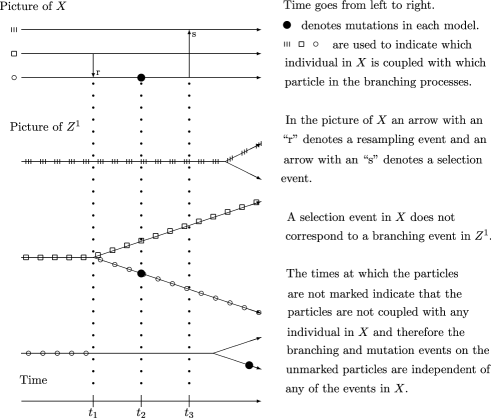
Figure 1: Picture of the coupling of $X$ with $Z^{1}$ when $N=3$.

Proposition 6

For any population size $N$, initial configuration $X_{0}$, time $t\geq 0$ and natural number $l$,

$$P(S_{t}\geq l)\leq\frac{N(t\mu)^{l}e^{t}}{l!}.$$

By Lemma 16 in the Appendix we have

$$P\bigl{(}M_{t}^{1}\geq l\bigr{)}\leq\frac{N(t\mu)^{l}e^{t}}{l!}$$

for any population size $N$, time $t\geq 0$ and natural number $l$. Note that from our notation above $Z^{1}$ is a Yule process with branching rate 1. To complete the proof we establish a coupling between $X$ and $Z^{1}$ such that for any population size $N$ and time $t\geq 0$ we have $M_{t}^{1}\geq S_{t}$. See Figure 1 for an illustration of the coupling. At all times every individual in $X$ will be paired with one particle in $Z^{1}$. The coupling is as follows:

• We initially have a one-to-one pairing of each individual $i$ in $X_{0}$ with each particle $i$ in $Z_{0}^{1}$.

• The particle in $Z^{1}$ that is paired with individual $i$ will increase in type by 1 only when individual $i$ gets a mutation.

• For each individual $i$ in $X$ and each $j\neq i$, individual $j$ is replaced by individual $i$ at rate $1/N$ due to resampling events. If individual $i$ replaces individual $j$ due to resampling, then the particle labeled $i$ in $Z^{1}$ branches. If particle $i$ has a higher type than particle $j$, then the new particle is paired with individual $j$. The particle that was paired with individual $j$ before the branching event is no longer paired with any individual in $X$. If particle $i$ has a lower type than particle $j$ then the particle that was paired with individual $j$ remains paired with individual $j$ and the new particle is not paired with any individual in $X$.

• The particle paired with individual $i$ in $Z^{1}$ branches at rate $1/N$ and these branching events are independent of any of the events in $X$. When the particle paired with individual $i$ branches due to these events, the new particle is not paired with any individual in $X$.

• Any particles in $Z^{1}$ that are not paired with an individual in $X$ branch and acquire mutations independently of $X$. The selection events in $X$ are independent of any events in $Z^{1}$.

Let $R^{i}$ be the type of the particle in $Z^{1}$ that is paired with individual $i$ and let

$$S_{s}^{i}=\sup_{0\leq r\leq s}\bigl{(}X_{0}^{-}-X_{r}^{i}\bigr{)}.$$

To show $M_{t}^{1}\geq S_{t}$ it is enough to show $R_{t}^{i}\geq S_{t}^{i}$ for all $i$. Initially $S_{0}^{i}\leq R_{0}^{i}=0$ for all $i$. Note that both $s\mapsto S_{s}^{i}$ and $s\mapsto R_{s}^{i}$ are increasing functions and that increases in these functions correspond to decreases in $X^{i}$.

When individual $i$ gets a mutation, $R^{i}$ increases by 1. However, if individual $i$ gets a mutation at time $s$, then $S^{i}$ will only increase by 1 if $S_{s-}^{i}=X_{0}^{-}-X_{s-}^{i}$ and the mutation is deleterious. Therefore, if individual $i$ gets a mutation at time $s$ and $S_{s-}^{i}\leq R_{s-}^{i}$, then

$$S_{s}^{i}\leq S_{s-}^{i}+1\leq R_{s^{-}}^{i}+1=R_{s}^{i}.$$

Suppose individual $j$ is replaced by individual $i$ due to a resampling event at time $s$ and that both $S_{s-}^{j}\leq R_{s-}^{j}$ and $S_{s-}^{i}\leq R_{s-}^{i}$ hold. With probability 1 we have $S_{s}^{i}=S_{s-}^{i}$ and $R_{s}^{i}=R_{s-}^{i}$. If $X_{0}^{-}-X_{s}^{i}\leq S_{s-}^{j}$ then $S_{s-}^{j}=S_{s}^{j}$. From this it follows that $S_{s}^{j}\leq R_{s}^{j}$. If $X_{0}^{-}-X_{s}^{i}>S_{s-}^{j}$ then $S_{s}^{j}=X_{0}^{-}-X_{s}^{i}\leq S_{s}^{i}\leq R_{s}^{i}$. If $R_{s}^{i}\geq R_{s-}^{j}$, then by the definition of the coupling, $R_{s}^{j}=R_{s}^{i}$. If $R_{s}^{i}<R_{s-}^{j}$, then by definition of the coupling, $R_{s}^{j}=R_{s-}^{j}$. Therefore, $R_{s}^{j}\geq R_{s}^{i}$ which gives us $S_{s}^{j}\leq R_{s}^{j}$.

Selection events will never increase $S^{i}$ and since $S^{i}$ and $R^{i}$ are increasing in time, a selection event at time $s$ will preserve the inequality $S_{s}^{i}\leq R_{s}^{i}$. This shows that any event that occurs at time $s$ which may change the fitness of an individual $i$ in $X$ will preserve the inequality $S_{s}^{i}\leq R_{s}^{i}$. Since the result holds for each individual $i$, we have $S_{t}\leq M_{t}^{1}$.

We now wish to bound the distance the front of the wave moves as a function of the initial width.

Proposition 7

For any initial configuration $X_{0}$, fixed time $t\geq 0$ and any integer $l\geq 0$, we have

$$P\Bigl{(}\sup_{0\leq s\leq t}D_{s}>l\Bigr{)}\leq\frac{2N(t\mu)^{l}e^{(\gamma(W_{0}+2l)+\mu+1)t}}{(l-1)!}.$$

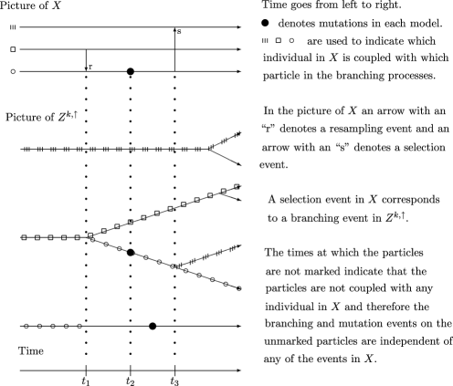
Recall that $W_{0}$ is the width of $X$ at time 0. We first establish a coupling between $X$ and $Z^{W_{0}+k,\uparrow}$ for each integer $k\geq 0$. See Figure 2 for an illustration of the coupling.

Figure 2: Picture of the coupling of $X$ with $Z^{k,\uparrow}$ when $N=3$.

Let $T^{k}=\inf\{t\dvtx S_{t}>k\}$ for $k\geq 1$. Every individual in $X$ will be paired with one particle in $Z^{W_{0}+k,\uparrow}$ until time $T^{k}$. We couple $Z^{W_{0}+k,\uparrow}$ with $X$ for all times $t\in[0,T^{k})$ as follows:

• We initially have a one-to-one pairing of each individual $i$ in $X_{0}$ with each particle $i$ in $Z_{0}^{W_{0}+k,\uparrow}$. When a particle in $Z_{t}^{W_{0}+k,\uparrow}$ is coupled with individual $i$, we refer to the particle as particle $i$.

• Particle $i$ increases in type by 1 only when individual $i$ gets a mutation.

• For each individual $i$ in $X$ and each $j\neq i$, individual $j$ is replaced by individual $i$ at rate $1/N$ due to resampling events. If individual $i$ replaces individual $j$ due to resampling, then particle $i$ branches. If particle $i$ has a higher type than particle $j$, then the new particle is paired with individual $j$. The particle that was paired with individual $j$ before the branching event is no longer paired with any individual in $X$. If particle $i$ has a lower type than particle $j$, then the particle that was paired with individual $j$ remains paired with individual $j$ and the new particle is not paired with any individual in $X$.

• Additionally, particle $i$ branches at rate $1/N$ and these branching events are independent of any of the events in $X$. When particle $i$ branches due to these events the new particle is not paired with any individual in $X$.

• In $X$ there is a time dependent rate $\gamma U_{s}^{i}$ at which individuals $j\neq i$ are replaced by individual $i$ due to selection events, namely,

  $$U_{s}^{i}=\frac{1}{N}\sum_{j=1}^{N}\bigl{(}X_{s}^{i}-X_{s}^{j}\bigr{)}^{+}.$$

  If individual $j$ is replaced by individual $i$ in $X$ due to a selection event, then particle $i$ branches. If particle $i$ has a higher type than particle $j$, then the new particle is paired with individual $j$. The particle that was paired with individual $j$ before the branching event is no longer paired with any individual in $X$. If particle $i$ has a lower type than particle $j$, then the particle that was paired with individual $j$ remains paired with individual $j$. The new particle is not paired with any individual in $X$.

• Additionally, particle $i$ branches at a time dependent rate $\gamma(R_{t}^{i,k}-U_{t}^{i})$ where $R_{t}^{i,k}$ is the type of particle $i$. These branching events are independent of any of the events in $X$. When such a branching event occurs, the new particle is not paired with any individual in $X$.

• Any particles in $Z^{W_{0}+k,\uparrow}$ that are not paired with an individual in $X$ branch and change type independently of $X$.

Fix $k\geq 1$. For the above coupling between $X$ and $Z^{W_{0}+k,\uparrow}$ to be well defined until time $T^{k}$, we need $R_{t}^{i,k}-U_{t}^{i}\geq 0$ for all $i\in\{1,\ldots,N\}$ and for all times $t\in[0,T^{k})$. Let $\overline{T}{}^{k,i}=\inf\{t\dvtx R_{t}^{i,k}-U_{t}^{i}<0\}$. The coupling between $X$ and $Z^{W_{0}+k,\uparrow}$ is well defined until time $\overline{T}{}^{k}=\min\{\overline{T}{}^{k,i}\dvtx 1\leq i\leq N\}$. We will show that $T^{k}\leq\overline{T}{}^{k}$.

Let

$$\overline{S}{}^{i}_{t}=\sup_{0\leq s\leq t}\bigl{(}X_{s}^{i}-X_{0}^{+}\bigr{)}\quad\mbox{and}\quad\overline{R}{}^{i,k}_{t}=R_{0}^{i,k}-W_{0}-k.$$

Initially $\overline{S}{}^{i}_{0}\leq\overline{R}{}^{i,k}_{0}=0$ for all $i$. Note that both $t\mapsto\overline{S}{}^{i}_{t}$ and $t\mapsto R_{t}^{i,k}$ are increasing functions, from which it follows that $t\mapsto\overline{R}{}^{i,k}_{t}$ is also an increasing function.

When individual $i$ gets a mutation, $\overline{R}{}^{i,k}$ increases by 1. However, if individual $i$ gets a mutation at time $s$ then $\overline{S}{}^{i}$ will only increase by 1 if $\overline{S}{}^{i}_{s-}=X_{s-}^{i}-X_{0}^{+}$ and the mutation is beneficial. Therefore, if individual $i$ gets a mutation at time $s$ and $\overline{S}{}^{i}_{s-}\leq\overline{R}{}^{i,k}_{s-}$, then

$$\overline{S}{}^{i}_{s}\leq\overline{S}{}^{i}_{s-}+1\leq\overline{R}{}^{i,k}_{s^{-}}+1=\overline{R}{}^{i,k}_{s}.$$

Suppose individual $j$ is replaced by individual $i$ due to a resampling or selection event at time $s$ and that both $\overline{S}{}^{j}_{s-}\leq\overline{R}{}^{j,k}_{s-}$ and $\overline{S}{}^{i}_{s}=\overline{S}{}^{i}_{s-}\leq\overline{R}{}^{i,k}_{s-}=\overline{R}{}^{i,k}_{s}$ hold. If $X_{s}^{i}-X_{0}^{+}\leq\overline{S}{}^{j}_{s-}$, then $\overline{S}{}^{j}_{s-}=\overline{S}{}^{j}_{s}$. It follows that $\overline{S}{}^{j}_{s}\leq\overline{R}{}^{j,k}_{s}$. If $X_{s}^{i}-X_{0}^{+}>\overline{S}{}^{j}_{s-}$ then $\overline{S}{}^{j}_{s}=X_{0}^{-}-X_{s}^{i}\leq\overline{S}{}^{i}_{s}\leq\overline{R}{}^{i,k}_{s}$. If $\overline{R}{}^{i,k}_{s}\geq\overline{R}{}^{j,k}_{s-}$, then by the definition of the coupling, $\overline{R}{}^{j,k}_{s}=\overline{R}{}^{i,k}_{s}$. If $\overline{R}{}^{i,k}_{s}<\overline{R}{}^{j,k}_{s-}$, then by definition of the coupling, $\overline{R}{}^{j,k}_{s}=\overline{R}{}^{j,k}_{s-}$. Therefore, $\overline{R}{}^{j,k}_{s}\geq\overline{R}{}^{i,k}_{s}$ which gives us $\overline{S}{}^{j}_{s}\leq\overline{R}{}^{j,k}_{s}$.

For any time $s<T^{k}$ we have $R^{i,k}_{s}\geq\overline{S}{}^{i}_{s}+W_{0}+k\geq X^{i}_{s}-X_{0}^{+}+W_{0}+k=X^{i}_{s}-X_{0}^{-}+k$. If there were $N$ individuals with fitness $X_{0}^{-}-k$ at time $s\in[0,\overline{T}{}^{k,i})$, then the rate at which individual $i$ replaces these $N$ individuals due to selection is $\gamma(X^{i}_{s}-X_{0}^{-}+k)$. However, for any time $s<T^{k}$, there are fewer than $N$ individuals being replaced by individual $i$ due to selection and they will all have fitnesses at least as large as $X_{0}^{-}-k$. This gives us a bound on the rate at which resampling events occur on individual $i$ before time $T^{k}$, namely, $U^{i}_{s}\leq X^{i}_{s}-X_{0}^{-}+k\leq R^{i,k}_{s}$ for all $s\in[0,T^{k})$. This shows that $T^{k}\leq\overline{T}{}^{k,i}$ for all $i$. Hence, $T^{k}\leq\overline{T}{}^{k}$ and the coupling is well defined until time $T^{k}$.

We have shown that any event that occurs at time $s\in[0,T^{k})$ which may change the fitness of an individual $i$ in $X$ will preserve the inequality $\overline{S}{}^{i}_{s}\leq\overline{R}{}^{i,k}_{s}$. Since the result holds for each individual $i$, for any $s\in[0,T^{k})$ we have

$$\sup_{0\leq r\leq s}D_{r}=\sup_{1\leq i\leq N}\overline{S}{}^{i}_{s}\leq\sup_{1\leq i\leq N}\overline{R}{}^{i,k}_{s}\leq M_{s}^{W_{0}+k,\uparrow}.$$

Note that if $\sup_{0\leq s\leq t}(X_{0}^{-}-X_{s}^{-})\leq k$ then $t<T^{k}$. On the event$\{\sup_{0\leq s\leq t}(X_{0}^{-}-X_{s}^{-})\leq k\}$ we have $M_{t}^{W_{0}+k,\uparrow}\geq\sup_{0\leq s\leq t}D_{s}$. This allows us to do the following computation:

$$P\Bigl{(}\sup_{0\leq s\leq t}D_{s}>l\Bigr{)} = \sum_{i=0}^{\infty}P\Bigl{(}\Bigl{\{}\sup_{0\leq s\leq t}D_{s}>l\Bigr{\}}\cap\Bigl{\{}\sup_{0\leq s\leq t}\bigl{(}X_{0}^{-}-X_{s}^{-}\bigr{)}=i\Bigr{\}}\Bigr{)}$$

$$\leq \sum_{i=0}^{\infty}P\Bigl{(}\bigl{\{}M_{t}^{W_{0}+i,\uparrow}>l\bigr{\}}\cap\Bigl{\{}\sup_{0\leq s\leq t}\bigl{(}X_{0}^{-}-X_{s}^{-}\bigr{)}=i\Bigr{\}}\Bigr{)}$$

$$\leq \sum_{i=0}^{\infty}P\Bigl{(}\bigl{\{}M_{t}^{W_{0}+i,\uparrow}>l\bigr{\}}\cap\Bigl{\{}\sup_{0\leq s\leq t}\bigl{(}X_{0}^{-}-X_{s}^{-}\bigr{)}\geq i\Bigr{\}}\Bigr{)}$$

$$\leq \sum_{i=0}^{\infty}P\bigl{(}M_{t}^{W_{0}+i,\uparrow}>l\bigr{)}\wedge P\Bigl{(}\sup_{0\leq s\leq t}\bigl{(}X_{0}^{-}-X_{s}^{-}\bigr{)}\geq i\Bigr{)}$$

$$\leq \sum_{i=0}^{\infty}P\bigl{(}M_{t}^{W_{0}+i,\uparrow}>l\bigr{)}\wedge\biggl{(}\frac{N(t\mu)^{i}e^{t}}{i!}\biggr{)}\qquad\mbox{by Proposition~{}\ref{BackSpeed}}$$

$$\leq \sum_{i=0}^{\infty}\biggl{(}\frac{N(t\mu)^{l}e^{(\gamma(W_{0}+i+l)+1)t}}{l!}\biggr{)}\wedge\biggl{(}\frac{N(t\mu)^{i}e^{t}}{i!}\biggr{)}$$

by Lemma 17 in the Appendix

$$\leq \frac{N(t\mu)^{l}e^{(\gamma(W_{0}+l)+1)t}}{l!}\sum_{i=0}^{l-1}e^{i\gamma t}+Ne^{t}\sum_{i=l}^{\infty}\frac{(t\mu)^{i}}{i!}$$

$$\leq \frac{N(t\mu)^{l}e^{(\gamma(W_{0}+l)+1)t}}{l!}\cdot le^{l\gamma t}+Ne^{t}\sum_{i=l}^{\infty}\frac{(t\mu)^{i}}{i!}$$

$$\leq \frac{N(t\mu)^{l}e^{(\gamma(W_{0}+2l)+1)t}}{(l-1)!}+\frac{N(t\mu)^{l}e^{(\mu+1)t}}{l!}$$

by Lemma 15 in the Appendix

$$\leq \frac{2N(t\mu)^{l}e^{(\gamma(W_{0}+2l)+\mu+1)t}}{(l-1)!}.$$

We now extend the bound we got on the least fit individuals in Proposition 6 to a slightly stronger result.

Definition 8.

Let $x\in\mathbb{Z}$ and let $\mathcal{S}_{t}^{x}\subset\{1,2,\ldots,N\}$ correspond to a collection of individuals at time $t$ which is determined by the following dynamics:

• Initially, $\mathcal{S}_{0}^{x}$ consists of all individuals whose fitness lies in the interval $(x,\infty)$.

• If a resampling or selection event occurs at time $t$ and an individual not in $\mathcal{S}_{t-}^{x}$ is replaced by a individual in $\mathcal{S}_{t-}^{x}$, then it is added to $\mathcal{S}_{t}^{x}$.

• If a beneficial mutation occurs at time $t$ on an individual not in $\mathcal{S}_{t-}^{x}$ that causes its fitness to increase from $x$ to $x+1$, it is added to $\mathcal{S}_{t}^{x}$.

• If a resampling event occurs at time $t$ to an individual in $\mathcal{S}_{t-}^{x}$ and it is replaced by a individual not in $\mathcal{S}_{t-}^{x}$, then it is removed from $\mathcal{S}_{t}^{x}$.

Mutation and selection events do not cause individuals to be lost from $\mathcal{S}^{x}$. We now prove the following corollary to Proposition 7.

Corollary 9

Let $A_{t}^{x,l}$ be the event that an individual in $\mathcal{S}_{s}^{x}$ has fitness in $(-\infty,x-l]$ for some time $s\in[0,t]$. For any initial configuration $X_{0}$, time $t\geq 0$ and any integer $l$,

$$P\bigl{(}A_{t}^{x,l}\bigr{)}\leq\frac{2N(t\mu)^{l}e^{(\gamma(W_{0}+2l)+\mu+1)t}}{(l-1)!}.$$

Note that we cannot use the bound found in Proposition 6 because individuals not in $\mathcal{S}_{t}^{x}$ may move to $\mathcal{S}_{t}^{x}$ due to selection events. In the proof of Proposition 6 the number of individuals with the least fitness cannot increase due to selection events. However, the number of individuals with the least fitness in $\mathcal{S}_{t}^{x}$ may increase due to selection events involving individuals not in $\mathcal{S}_{t}^{x}$. Proof of Corollary 9 For $k\geq 1$ let $X$ be coupled with $Z^{W_{0}+k,\uparrow}$ as in the proof of Proposition 7. Let $T^{k}$, $R^{i,k}_{t}$ and $\overline{R}{}^{i,k}_{t}$ be defined as they were in the proof of Proposition 7. Define $\overline{T}{}^{i}_{s}=\{r\in[0,s]\dvtx i\in\mathcal{S}_{r}^{x}\}$ and let

$$S^{i}_{s}=\cases{\displaystyle\sup_{r\in\overline{T}{}^{i}_{s}}\bigl{(}x-X_{r}^{i}\bigr{)},&\quad if $\overline{T}{}^{i}_{s}\neq\varnothing$,\vspace*{2pt}\cr-\infty,&\quad if $\overline{T}{}^{i}_{s}=\varnothing$.}$$

The goal is to show that for all $s\in[0,T^{k})$ we have

$$\sup_{1\leq i\leq N}S^{i}_{s}\leq\sup_{1\leq i\leq N}\overline{R}{}^{i,k}_{s}\leq M_{s}^{W_{0}+k,\uparrow}.$$

Note that we can only consider the coupling of $X$ with $Z^{W_{0}+k,\uparrow}$ until time $T^{k}$ because after this time the coupling is not well defined.

Initially all of the individuals in $\mathcal{S}_{0}^{x}$ have fitness in $(x,\infty)$. Therefore, if $i\in\mathcal{S}_{0}^{x}$ then $S_{0}^{i}\leq 0=\overline{R}{}^{i,k}_{0}$. If $i\notin\mathcal{S}_{0}^{x}$ then $S_{0}^{i}=-\infty<\overline{R}{}^{i,k}_{0}$.

Suppose individual $i$ gets a mutation at time $s$ and that for any time $s^{\prime}\in[0,s-)$ we have $S_{s^{\prime}}^{i}\leq\overline{R}{}^{i,k}_{s^{\prime}}$. Then $\overline{R}{}^{i,k}$ increases by 1. If $i\in\overline{S}{}^{x}_{s-}$ then $S^{i}_{s}$ will only increase by 1 if $S_{s-}^{i}=x-X^{i}_{s}$ and the mutation is deleterious. If $i\notin\mathcal{S}_{s-}^{x}$ and the mutation does not cause the fitness of individual $i$ to change from $x$ to $x+1$, then $S^{i}_{s}=S_{s-}^{i}$. If $i\notin\mathcal{S}_{s-}^{x}$ and the mutation does cause the fitness of individual $i$ to change from $x$ to $x+1$, then $S^{i}_{s}=S_{s-}^{i}\vee 0$. In any of these three cases, $S^{i}_{s}\leq\overline{R}{}^{i,k}_{s}$.

Suppose individual $j$ is replaced by individual $i$ due to a resampling or selection event at time $s$ and that $S_{s-}^{j}\leq\overline{R}{}^{j,k}_{s-}$ and $S_{s-}^{i}\leq\overline{R}{}^{i,k}_{s-}$. If $i\notin\overline{S}{}^{x}_{s-}$ then $S_{s-}^{j}=S_{s}^{j}\leq\overline{R}{}^{j,k}_{s-}$. Suppose $i\in\mathcal{S}_{s-}^{x}$. If $x-X^{i}_{s}\leq S_{s-}^{j}$ then $S_{s-}^{j}=S_{s}^{j}$. From this it follows that $S_{s}^{j}\leq\overline{R}{}^{j}_{s}$. If $x-X^{i}_{s}>S_{s-}^{j}$, then $S_{s}^{j}=x-X^{i}_{s}\leq S^{i}_{s}\leq\overline{R}{}^{i}_{s}$. If $\overline{R}{}^{i}_{s}\geq\overline{R}{}^{j}_{s-}$, then by the definition of the coupling, $\overline{R}{}^{j}_{s}=\overline{R}{}^{i}_{s}$. If $\overline{R}{}^{i}_{s}<\overline{R}{}^{j}_{s-}$, then by definition of the coupling, $\overline{R}{}^{j}_{s}=\overline{R}{}^{j}_{s-}$. Therefore, $\overline{R}{}^{j}_{s}\geq\overline{R}{}^{i}_{s}$ which gives us $S^{j}_{s}\leq\overline{R}{}^{j}_{s}$.

Note that if $\sup_{0\leq s\leq t}(X_{0}^{-}-X_{s}^{-})\leq k$ then $t<T^{k}$. Therefore, on the event $\{\sup_{0\leq s\leq t}(X_{0}^{-}-X_{s}^{-})\leq k\}$ we have $M^{W_{0}+k,\uparrow}_{t}\geq\sup_{1\leq i\leq N}S^{i}_{s}$. This allows us to do the following computation:

$$P\Bigl{(}\sup_{0\leq s\leq t}\sup_{1\leq i\leq N}S^{i}_{s}>l\Bigr{)}$$

$$\qquad=\sum_{i=0}^{\infty}P\Bigl{(}\Bigl{\{}\sup_{0\leq s\leq t}\sup_{1\leq i\leq N}S^{i}_{s}>l\Bigr{\}}\cap\Bigl{\{}\sup_{0\leq s\leq t}\bigl{(}X_{0}^{-}-X_{s}^{-}\bigr{)}=i\Bigr{\}}\Bigr{)}$$

$$\qquad\leq\sum_{i=0}^{\infty}P\Bigl{(}\bigl{\{}M_{t}^{W_{0}+i,\uparrow}>l\bigr{\}}\cap\Bigl{\{}\sup_{0\leq s\leq t}\bigl{(}X_{0}^{-}-X_{s}^{-}\bigr{)}=i\Bigr{\}}\Bigr{)}.$$

This is the same bound as equation (3) in the proof of Proposition 7. Therefore, we have established the same bound. Proof of Proposition 3 By definition $D_{\mathcal{T}}^{\prime}$ has the same distribution as $M_{\mathcal{T}}^{\mathcal{W},\uparrow}$ so by Lemma 17 in the Appendix we have

$$P\bigl{(}D_{\mathcal{T}}^{\prime}>l\bigr{)}\leq\frac{N(\mathcal{T}\mu)^{l}e^{(\gamma(\mathcal{W}+l)+1)\mathcal{T}}}{l!}.$$

Then

$$\frac{E[D_{\mathcal{T}}^{\prime}]}{2\mathcal{W}} = \frac{1}{2\mathcal{W}}\sum_{l=0}^{\infty}P\bigl{(}D_{\mathcal{T}}^{\prime}>l\bigr{)}$$

$$\leq \frac{1}{2\mathcal{W}}\Biggl{[}2\mathcal{W}+\sum_{l=2\mathcal{W}}^{\infty}\frac{N(\mathcal{T}\mu)^{l}e^{(\gamma(\mathcal{W}+l)+1)\mathcal{T}}}{l!}\Biggr{]}.$$

By Lemma 15 in the Appendix we have

$$\sum_{l=2\mathcal{W}}^{\infty}\frac{N(\mathcal{T}\mu)^{l}e^{(\gamma(\mathcal{W}+l)+1)\mathcal{T}}}{l!}\leq\frac{Ne^{(\gamma\mathcal{W}+1)\mathcal{T}}(\mathcal{T}\mu e^{\gamma\mathcal{T}})^{2\mathcal{W}}e^{\mathcal{T}\mu e^{\gamma\mathcal{T}}}}{(2\mathcal{W})!}.$$ (3)

Note that for any $k\geq 2$ both $D_{k\mathcal{T}}^{\prime}-D_{(k-1)\mathcal{T}}^{\prime}$ and $D_{\mathcal{T}}^{\prime}$ have the same distribution, namely, that of $M_{\mathcal{T}}^{\mathcal{W}}$. Choose $t\in[k\mathcal{T},(k+1)\mathcal{T})$ for some $k\geq 1$. Because $D_{t}^{\prime}$ is increasing in $t$ we have

$$\frac{D_{t}^{\prime}}{t}\leq\frac{1}{k\mathcal{T}}\bigl{(}D_{(k+1)\mathcal{T}}^{\prime}-D_{k\mathcal{T}}^{\prime}+D_{k\mathcal{T}}^{\prime}-\cdots+D_{2\mathcal{T}}^{\prime}-D_{\mathcal{T}}^{\prime}+D_{\mathcal{T}}^{\prime}\bigr{)}.$$

Therefore,

$$\frac{E[D_{t}^{\prime}]}{t}\leq\frac{(k+1)E[D_{\mathcal{T}}^{\prime}]}{k\mathcal{T}}\leq\frac{2E[D_{\mathcal{T}}^{\prime}]}{\mathcal{T}}.$$

Let $t>\mathcal{T}$. Dividing both sides by $2\mathcal{W}/\mathcal{T}$ and using the bounds found in equations (3) and (3) gives us

$$\frac{\mathcal{T}E[D_{t}^{\prime}]}{2t\mathcal{W}}\leq\frac{2E[D_{\mathcal{T}}^{\prime}]}{2\mathcal{W}}\leq 2+\frac{Ne^{(\gamma\mathcal{W}+1)\mathcal{T}}(\mathcal{T}\mu e^{\gamma\mathcal{T}})^{2\mathcal{W}}e^{\mathcal{T}\mu e^{\gamma\mathcal{T}}}}{2\mathcal{W}(2\mathcal{W})!}.$$

By Stirling’s formula we have

$$\frac{Ne^{(\gamma\mathcal{W}+1)\mathcal{T}}(\mathcal{T}\mu e^{\gamma\mathcal{T}})^{2\mathcal{W}}e^{\mathcal{T}\mu e^{\gamma\mathcal{T}}}}{2\mathcal{W}(2\mathcal{W})!}\sim\frac{Ne^{(\gamma\mathcal{W}+1)\mathcal{T}}(\mathcal{T}\mu e^{\gamma\mathcal{T}})^{2\mathcal{W}}e^{\mathcal{T}\mu e^{\gamma\mathcal{T}}+2\mathcal{W}}}{(2\mathcal{W})^{2\mathcal{W}+1}\sqrt{4\pi\mathcal{W}}}=e^{x},$$

where

$$x = \log N+\mathcal{T}\bigl{(}\gamma\mathcal{W}+1+\mu e^{\gamma\mathcal{T}}\bigr{)}+2\mathcal{W}\bigl{(}\log\bigl{(}\mathcal{T}\mu e^{\gamma\mathcal{T}}\bigr{)}+1\bigr{)}$$

$${}-(2\mathcal{W}+1)\log(2\mathcal{W})-\log(4\pi\mathcal{W})/2.$$

As $N\rightarrow\infty$ we have $x\sim-(2\mathcal{W}+1)\log(2\mathcal{W})\sim-2w\log N$. Therefore,

$$\frac{\mathcal{T}E[D_{t}^{\prime}]}{2t\mathcal{W}}\leq 3$$

for $N$ large enough. Proof of Proposition 2 We now couple $X$ with $X^{\prime}$ by coupling $X$ with the sequence of processes $\{\mathcal{Z}^{m}\}_{m=0}^{\infty}$. Let

$$I_{m}=\bigl{(}m\mathcal{T},(m+1)\mathcal{T}\bigr{]}\cap\bigcup_{n=1}^{\infty}[t_{n},s_{n})\quad\mbox{and}\quad J_{m}=(0,\mathcal{T}]\cap\bigcup_{n=1}^{\infty}[t_{n}-m\mathcal{T},s_{n}-m\mathcal{T}).$$

For any $m\geq 0$ we couple $X$ and $\mathcal{Z}^{m}$ as follows:

• The particles in $\mathcal{Z}_{0}^{m}$ are labeled $1,2,\ldots,N$.

• For any time in $I_{m}^{C}$ the process $X$ behaves independently of $\mathcal{Z}^{m}$. For any time in $J_{m}^{C}$ the process $\mathcal{Z}^{m}$ behaves independently of the process $X$. During the time $J_{m}^{C}$, if a particle labeled $i$ in $\mathcal{Z}^{m}$ branches, the particle remains labeled $i$ and the new particle is unlabeled.

• The particle in $\mathcal{Z}^{m}$ that is paired with individual $i$ will increase in type by 1 at time $t\in J_{m}$ only when individual $i$ gets a mutation at time $t+m\mathcal{T}\in I_{m}$.

• For each individual $i$ in $X$ and each $j\neq i$, individual $j$ is replaced by individual $i$ at rate $1/N$ due to resampling events. If individual $i$ replaces individual $j$ due to resampling at time $t\in I_{m}$, then the particle labeled $i$ in $\mathcal{Z}^{m}$ branches at time $t-m\mathcal{T}\in J_{m}$. If particle $i$ has a higher type than particle $j$, then the new particle is paired with individual $j$. The particle that was paired with individual $j$ before the branching event is no longer paired with any individual in $X$. If particle $i$ has a lower type than particle $j$, then the particle that was paired with individual $j$ remains paired with individual $j$ and the new particle is not paired with any individual in $X$.

• The particle paired with individual $i$ in $\mathcal{Z}^{m}$ branches at rate $1/N$ for all times $t\in J_{m}$ and these branching events are independent of any of the events in $X$. When the particle paired with individual $i$ branches due to these events the new particle is not paired with any individual in $X$.

• In $X$ there is a time dependent rate $\gamma U^{i}_{s}$ at which individuals $j\neq i$ are replaced by individual $i$ due to selection events. If individual $j$ is replaced by individual $i$ in $X$ due to a selection event at time $t\in I_{m}$, then the particle labeled $i$ in $\mathcal{Z}^{m}$ splits at time $t-m\mathcal{T}\in J_{m}$. If particle $i$ has a higher type than particle $j$, then the new particle is paired with individual $j$. The particle that was paired with individual $j$ before the branching event is no longer paired with any individual in $X$. If particle $i$ has a lower type than particle $j$, then the particle that was paired with individual $j$ remains paired with individual $j$. The new particle is not paired with any individual in $X$.

• A particle labeled $i$ in $\mathcal{Z}^{m}$ splits at a time-dependent rate $\gamma(R^{i,k}_{t}-U_{t}^{i})$ for all times $t\in J_{m}$ where $R^{i,k}_{t}$ is the type of particle $i$. These branching events are independent of any of the events in $X$. When such a branching event occurs, the new particle is not paired with any individual in $X$.

• Any particles in $\mathcal{Z}^{m}$ that are not paired with an individual in $X$ branch and acquire mutations independently of $X$.

Observe the following bound for $D_{t}$:

$$D_{t} \leq \sum_{i=1}^{N_{t}-1}(D_{t_{i+1}}-D_{s_{i}})+\sum_{i=1}^{N_{t}}(D_{s_{i}}-D_{t_{i}})+\sup_{s_{N_{t}}\leq s\leq t_{N_{t}+1}}(D_{s}-D_{s_{N_{t}}})$$

$${}+\sup_{t_{N_{t}+1}\leq s\leq t}(D_{s}-D_{t_{N_{t}+1}}),$$

where we consider the supremum over the empty set to be 0. By definition we have

$$\sum_{i=1}^{N_{t}-1}(D_{t_{i+1}}-D_{s_{i}})+\sup_{s_{N_{t}}\leq s\leq t_{N_{t}+1}}(D_{s}-D_{s_{N_{t}}})\leq\sum_{i=1}^{N_{t}}Y_{i}.$$

To finish the proof we will show

$$\sum_{i=1}^{N_{t}}\sup_{t_{i}\leq s\leq s_{i}}(D_{s}-D_{t_{i}})+\sup_{t_{N_{t}+1}\leq s\leq t}(D_{s}-D_{t_{N_{t}+1}})\leq D_{t}^{\prime}.$$

To do this we define

$$M_{t}=\sum_{i=1}^{N_{t}}\sup_{t_{i}\leq s\leq s_{i}}(D_{s}-D_{t_{i}})+\sup_{t_{N_{t}+1}\leq s\leq t}(D_{s}-D_{t_{N_{t}+1}})$$

for all times $t\geq 0$. Suppose $M_{s}\leq D_{s}^{\prime}$ for all $s\in[0,t)$ and a mutation, resampling or selection event occurs in $X$ at time $t$. If $t\in(s_{i},t_{i+1})$ for some $i\geq 0$, then $M_{t-}=M_{t}$ because the process $M$ does not change on these time intervals. It is possible that $D_{t}^{\prime}$ changes, but $D_{t}^{\prime}$ can only increase. Therefore, $D_{t}^{\prime}\geq M_{t}$. If $t\in[t_{i},s_{i}]\cap(m\mathcal{T},(m+1)\mathcal{T}]$ for some $i\geq 0$ and $m\geq 0$, then at time $t$ the processes $X$ and $X^{\prime}$ are coupled. More precisely, $X$ and $\mathcal{Z}^{m}$ are coupled and the coupling has the same dynamics as the coupling in Proposition 7 except the time shift. The same argument used in Proposition 7 shows that $D_{t}^{\prime}\geq M_{t}$ whether the individual changed fitness due to mutation, resampling or selection. Since this inequality is preserved on any event that may change $M_{t}$, it is true for all times $t$.

4 Bounding the rate when the width is large

We consider what happens when the width is large in this section. By large width we mean $W_{t}\geq\mathcal{W}$. The statements in this section are easier to make when we consider an initial configuration of $X$ such that $W_{0}\geq\mathcal{W}$. Although the conditions of Theorem 1 state that $W_{0}=0$, we can wait for a random time $\tau$ so that $W_{\tau}\geq\mathcal{W}$ and apply the strong Markov property.

We begin this section by showing that when the width is large enough the selection mechanism will cause the width to decrease quickly. We give a labeling to the individuals that will help us in this regard. Define the following subsets of $\mathbb{R}$:

We will label each individual in $X_{0}$ with two labels. For the first labeling, we use $\mathfrak{a}$ to label the individuals in $I_{1}\cup I_{2}$, we use $\mathfrak{b}$ to label the individuals in $I_{3}$ and we use $\mathfrak{c}$ to label the individuals in $I_{4}$. For the second labeling we use $\mathfrak{a}^{\prime}$ to label the individuals in $I_{1}$, we use $\mathfrak{b}^{\prime}$ to label the individuals in $I_{2}$ and we use $\mathfrak{c}^{\prime}$ to label the individuals in $I_{3}\cup I_{4}$.

Let $\mathfrak{A}_{t}$, $\mathfrak{B}_{t}$ and $\mathfrak{C}_{t}$ denote the number of individuals labeled $\mathfrak{a}$, $\mathfrak{b}$ and $\mathfrak{c}$ at time $t$, respectively. Let $\mathfrak{A}_{t}^{\prime}$, $\mathfrak{B}_{t}^{\prime}$ and $\mathfrak{C}_{t}^{\prime}$ denote the number of individuals labeled $\mathfrak{a}^{\prime}$, $\mathfrak{b}^{\prime}$ and $\mathfrak{c}^{\prime}$ at time $t$, respectively.

The individuals change labels over time according to the following dynamics:

• Mutations: If the fitness of an individual labeled $\mathfrak{a}$ increases so that it is in $I_{3}$, then the individual is relabeled $\mathfrak{b}$. If the fitness of a individual labeled $\mathfrak{a}^{\prime}$ increases so that it is in $I_{2}$, then the individual is relabeled $\mathfrak{b}^{\prime}$. Likewise, if the fitness of a individual labeled $\mathfrak{b}$ increases so that it is in $I_{4}$, then it is relabeled $\mathfrak{c}$ and if the fitness of a individual labeled $\mathfrak{b}^{\prime}$ increases so that it is in $I_{3}$, then it is relabeled $\mathfrak{c}^{\prime}$. Deleterious mutations do not cause individuals to be relabeled.

• Resampling: Any resampling event in which individual $i$ is replaced by individual $j$ causes individual $i$ to inherit the labels of individual $j$.

• Selection: If an individual labeled $\mathfrak{a}$ is replaced due to a selection event, it inherits the corresponding label of the individual that replaced it. If an individual labeled $\mathfrak{a}^{\prime}$ is replaced due to a selection event, it inherits the corresponding label of the individual that replaced it. If an individual labeled $\mathfrak{b}$ is replaced by an individual labeled $\mathfrak{c}$ due to a selection event, then the individual that was labeled $\mathfrak{b}$ is relabeled $\mathfrak{c}$. If an individual labeled $\mathfrak{b}^{\prime}$ is replaced by an individual labeled $\mathfrak{c}^{\prime}$ due to a selection event, then the individual that was labeled $\mathfrak{b}^{\prime}$ is relabeled $\mathfrak{c}^{\prime}$. Any other selection events do not cause the labels of the individuals to be changed.

Let $A_{1}$ be the event that there is an individual labeled $\mathfrak{b}$ with fitness in $(-\infty,X_{0}^{+}-\frac{5}{32}W_{0})$ for some time $t\in[0,\mathcal{T}]$. Let $A_{2}$ be the event that there is an individual labeled $\mathfrak{c}$ with fitness in $(-\infty,X_{0}^{+}-\frac{3}{32}W_{0})$ for some time $t\in[0,\mathcal{T}]$. Let $A_{1}^{\prime}$ be the event that there is an individual labeled $\mathfrak{b}^{\prime}$ with fitness in $(-\infty,X_{0}^{+}-\frac{7}{32}W_{0})$ for some time $t\in[0,\mathcal{T}]$. Let $A_{2}^{\prime}$ be the event that there is an individual labeled $\mathfrak{c}^{\prime}$ with fitness in $(-\infty,X_{0}^{+}-\frac{5}{32}W_{0})$ for some time $t\in[0,\mathcal{T}]$.

Lemma 10

Suppose $W_{0}\geq\mathcal{W}$ for all $N$. Then

$$P\bigl{(}A_{1}\cup A_{2}\cup A_{1}^{\prime}\cup A_{2}^{\prime}\bigr{)}\rightarrow 0\qquad\mbox{as }N\rightarrow\infty.$$

First we show the result for $A_{1}$. We apply Corollary 9 with $x=X_{0}^{+}-2W_{0}/16$, $t=t_{0}$ and $l=W_{0}/32$. Recall that we had defined $\mathcal{S}_{t}^{x}$ in Definition 8. Because $x=X_{0}^{+}-2W_{0}/16$, we have that $\mathcal{S}_{0}^{x}$ consists of all the individuals labeled $\mathfrak{b}$ or $\mathfrak{c}$. Setting $t=\mathcal{T}$ and $l=W_{0}/32$ will make $A_{t}^{x,l}$ the event that an individual labeled $\mathfrak{b}$ or $\mathfrak{c}$ has fitness less than $X_{0}^{+}-\frac{5}{32}W_{0}$ by time $\mathcal{T}$. Note that according to the relabeling dynamics, individual $i$ being labeled $\mathfrak{b}$ or $\mathfrak{c}$ is equivalent to $i\in\mathcal{S}^{x}$. Therefore, $A_{1}\subset A_{t}^{x,l}$ and we get

$$P(A_{1})\leq P\bigl{(}A_{t}^{l}\bigr{)}\leq\frac{2N(t\mu)^{l}e^{(\gamma(W_{0}+2l)+\mu+1)t}}{\lfloor l-1\rfloor!}.$$

Applying Stirling’s formula we have

$$\frac{2N(t\mu)^{l}e^{(\gamma(W_{0}+2l)+\mu+1)t}}{\lfloor l-1\rfloor!}\sim\frac{2N(t\mu)^{l}e^{(\gamma(W_{0}+2l)+\mu+1)t+\lfloor l-1\rfloor}}{\lfloor l-1\rfloor^{\lfloor l-1\rfloor}\sqrt{2\pi\lfloor l-1\rfloor}}=e^{x},$$

where

$$x = \log(2N)+l\log(t\mu)+\bigl{(}\gamma(W_{0}+2l)+\mu+1\bigr{)}t+\lfloor l-1\rfloor$$

$${}-\lfloor l-1\rfloor\log\bigl{(}\lfloor l-1\rfloor\bigr{)}-\log\bigl{(}2\pi\lfloor l-1\rfloor\bigr{)}/2.$$

As $N\rightarrow\infty$ we have $x\sim-\lfloor l-1\rfloor\log(\lfloor l-1\rfloor)\sim-w\log N/32$. Therefore,

$$P(A_{1})\rightarrow 0\qquad\mbox{as }N\rightarrow\infty.$$

We can apply Corollary 9 with $x=X_{0}^{+}-W_{0}/16$, $t=\mathcal{T}$ and $l=W_{0}/32$ to get the same bound for $P(A_{2})$. By choosing $x$, $t$ and $l$ in this way, the event $A_{t}^{x,l}$ is the event that an individual labeled $\mathfrak{c}$ has fitness less than $X^{+}(0)-\frac{3}{32}W_{0}$ by time $\mathcal{T}$. This shows that $P(A_{2})$ also tends to 0 as $N$ tends to infinity.

Likewise, to show $P(A_{1}^{\prime})$ tends to 0 as $N$ goes to infinity we can apply Corollary 9 with $x=X_{0}^{+}-\frac{3}{16}W_{0}$, $t=\mathcal{T}$ and $l=W_{0}/32$, and to show $P(A_{2}^{\prime})$ tends to 0 as $N$ goes to infinity we can apply Corollary 9 with $x=X_{0}^{+}-\frac{2}{16}W_{0}$, $t=\mathcal{T}$ and $l=W_{0}/32$.

Lemma 11

Suppose $W_{0}\geq\mathcal{W}$ for all $N$. Let $T$ be a stopping time whose definition may depend on $N$ such that $\mathfrak{C}_{T}^{\prime}\geq N/4$ for all $N$. Let $B_{T}=\inf\{t\geq T\dvtx X_{t}^{-}>X_{0}^{+}-W_{0}/4\}$. Then

$$P\bigl{(}B_{T}1_{\{T<\mathcal{T}/2\}}>\tfrac{1}{2}\mathcal{T}\bigr{)}\rightarrow 0\qquad\mbox{as }N\rightarrow\infty.$$

Let $A_{3}^{\prime}$ be the event that $\mathfrak{C}_{t}^{\prime}\geq N/5$ for all times $t\in[T,T+\frac{1}{2}\mathcal{T})$. The only way for an individual labeled $\mathfrak{c}^{\prime}$ to change its label is for it to be replaced by an individual labeled $\mathfrak{a}^{\prime}$ or $\mathfrak{b}^{\prime}$ via a resampling event. The rate at which individuals marked $\mathfrak{c}^{\prime}$ undergo resampling events with individuals marked $\mathfrak{a}^{\prime}$ or $\mathfrak{b}^{\prime}$ at time $t$ is

$$\frac{\mathfrak{C}_{t}^{\prime}(N-\mathfrak{C}_{t}^{\prime})}{N}\leq\frac{N}{4}.$$

Let $\{U_{n}\}_{n=0}^{\infty}$ be a simple random walk with $U_{0}=N/4\leq\mathfrak{C}_{T}^{\prime}$. Let $T\leq t_{1}<t_{2}<\cdots$ be the times at which individuals labeled $\mathfrak{c}^{\prime}$ are involved in resampling events with individuals that are not labeled $\mathfrak{c}^{\prime}$ after time $T$. We couple $\{U_{n}\}_{n=0}^{\infty}$ with $X$ so that if at time $t_{n}$ an individual is labeled $\mathfrak{c}^{\prime}$ due to a resampling event, then $U_{n}=U_{n-1}+1$. If at time $t_{n}$ an individual loses the label $\mathfrak{c}^{\prime}$ due to a resampling event, then $U_{n}=U_{n-1}-1$. To have $U_{m}<N/5$ for some $m$ satisfying $0\leq m\leq n$ we will need ${\max_{0\leq m\leq n}}|U_{m}-U_{0}|\geq N/20$. It follows from the reflection principle that there exists a constant $C$ such that $E[{\max_{0\leq m\leq n}}|U_{m}-U_{0}|]\leq C\sqrt{n}$ for all $n\geq 0$. By Markov’s inequality,

$$P\Bigl{(}\max_{0\leq m\leq n}|U_{m}-U_{0}|\geq N/20\Bigr{)}\leq C\sqrt{n}/N$$

for some constant $C$.

Let $R$ be the number of resampling events that occur in the time interval $[T,T+\frac{1}{2}\mathcal{T})$ that involve pairs of individuals such that one is labeled $\mathfrak{c}^{\prime}$ and the other is not. Using Lemma 15 in the Appendix and the fact that the rate at which resampling events occur is bounded above by $N/4$, we have

$$P(R>k)\leq\sum_{i=k+1}^{\infty}\frac{(N\mathcal{T})^{i}e^{-N\mathcal{T}/8}}{8^{i}i!}\leq\frac{(N\mathcal{T})^{k}}{8^{k}k!}.$$

Then

$$P\bigl{(}\bigl{(}A_{3}^{\prime}\bigr{)}^{C}\bigr{)} \leq P\Bigl{(}\Bigl{\{}\max_{0\leq m\leq R}|U_{m}-U_{0}|\geq N/20\Bigr{\}}\cap\bigl{\{}R\leq N^{3/2}\bigr{\}}\Bigr{)}$$

$${}+P\Bigl{(}\Bigl{\{}\max_{0\leq m\leq R}|U_{m}-U_{0}|\geq N/20\Bigr{\}}\cap\bigl{\{}R>N^{3/2}\bigr{\}}\Bigr{)}$$

$$\leq P\Bigl{(}\Bigl{\{}\max_{0\leq m\leq N^{3/2}}|U_{m}-U_{0}|\geq N/20\Bigr{\}}\Bigr{)}+P\bigl{(}R>N^{3/2}\bigr{)}$$

$$\leq \frac{C}{N^{1/4}}+\frac{(N\mathcal{T})^{N^{3/2}}}{8^{N^{3/2}}\lceil N^{3/2}\rceil!}$$

$$\rightarrow 0\qquad\mbox{as }N\rightarrow\infty.$$

Let $A_{4}^{\prime}$ be the event that $\mathfrak{A}_{t}^{\prime}=0$ for some time $t\in[T,T+\frac{1}{2}\mathcal{T})$. Notice that if $\mathfrak{A}_{t}^{\prime}=0$, then $\mathfrak{A}_{s}^{\prime}=0$ for $s\geq t$. Therefore, $A_{4}^{\prime}$ is the event that the label $\mathfrak{a}^{\prime}$ is eliminated by time $T+\frac{1}{2}\mathcal{T}$. By the given dynamics, $\mathfrak{A}_{t}^{\prime}$ can only increase when individuals marked $\mathfrak{a}^{\prime}$ replace individuals marked $\mathfrak{b}^{\prime}$ or $\mathfrak{c}^{\prime}$ via resampling events. At time $t$ the rate at which this happens is

$$\frac{1}{2}\cdot\frac{\mathfrak{A}_{t}^{\prime}(N-\mathfrak{A}_{t}^{\prime})}{N}\leq\mathfrak{A}_{t}^{\prime}.$$ (5)

We define the event $\mathcal{E}$ as

$$\mathcal{E}=\bigl{(}A_{1}^{\prime}\bigr{)}^{C}\cap\bigl{(}A_{2}^{\prime}\bigr{)}^{C}\cap A_{3}^{\prime}\cap\bigl{\{}T<\tfrac{1}{2}\mathcal{T}\bigr{\}}.$$

Selection will cause $\mathfrak{A}^{\prime}$ to decrease. On the event $(A_{2}^{\prime})^{C}$ all of the individuals marked $\mathfrak{c}^{\prime}$ will have fitness at least $\frac{1}{32}W_{0}$ greater than any individual marked $\mathfrak{a}$ until time $t_{0}$. Thus, on the event $(A_{2}^{\prime})^{C}\cap\{T<\frac{1}{2}t_{0}\}$, all of the individuals marked $\mathfrak{c}^{\prime}$ will have fitness at least $\frac{1}{32}W_{0}$ greater than any individual marked $\mathfrak{a}$ for all times $t\in[T,T+\frac{1}{2}\mathcal{T})$. On the event $A_{3}^{\prime}$ there are at least $N/5$ individuals marked $\mathfrak{c}$ for all times $t\in[T,T+\frac{1}{2}\mathcal{T})$. Hence, on the event $\mathcal{E}$ individuals marked $\mathfrak{a}^{\prime}$ will become individuals marked $\mathfrak{c}^{\prime}$ by a rate of at least

$$\frac{\gamma\mathfrak{A}_{t}^{\prime}\mathfrak{C}_{t}^{\prime}W_{0}}{32N}\geq\frac{\gamma}{160}W_{0}\mathfrak{A}_{t}^{\prime}$$ (6)

for all times $t\in[T,T+\frac{1}{2}\mathcal{T})$.

Let $\{U_{n}^{\prime}\}$ be a biased random walk which goes up with probability

$$p^{\prime}=\frac{160}{160+\gamma W_{0}}$$

and down with probability $1-p^{\prime}$. Let $N$ be large enough so that $p^{\prime}<1/2$. Because the random walk is biased downward, the probability that the random walk visits a state $j<U_{0}^{\prime}$ is 1. Once the random walk is in state $j$, it goes up 1 with probability $p^{\prime}$ and will eventually return to $j$ with probability 1. The random walk will go down 1 with probability $1-p^{\prime}$ and, from basic martingale arguments, the probability that it never returns to $j$ again is $(1-2p^{\prime})/(1-p^{\prime})$. Therefore, once $U^{\prime}$ is in state $j$, the probability it never returns to state $j$ is

$$\frac{(1-2p^{\prime})}{1-p^{\prime}}\cdot\bigl{(}1-p^{\prime}\bigr{)}=1-2p^{\prime}.$$

Hence, the number of times $U^{\prime}$ visits a state $j<U_{0}^{\prime}$ has the geometric distribution with mean $1/(1-2p^{\prime})$. For more details see DNA , pages 194–196.

By equations (5) and (6) we see that on the event $\mathcal{E}$, if $\mathfrak{A}^{\prime}$ changes during the time interval $[T,T+\frac{1}{2}\mathcal{T})$, it decreases with probability higher than $p^{\prime}$. The expected number of times that $\mathfrak{A}^{\prime}$ will visit state $j$ is therefore less than or equal to $1/(1-2p^{\prime})$ for any $j\in\{1,2,\ldots,N-1\}$. Also, the rate at which $\mathfrak{A}_{t}^{\prime}$ changes state is at least

$$\frac{\gamma}{160}W_{0}\mathfrak{A}_{t}^{\prime}$$

for all times $t\in[T,T+\frac{1}{2}\mathcal{T})$ by equation (6). Let $\overline{A}=\{t\geq T\dvtx\mathfrak{A}_{t}^{\prime}>0\}$ and let $\lambda$ be Lebesgue measure. Then

$$E\bigl{[}\lambda(\overline{A})1_{\mathcal{E}}\bigr{]}\leq\frac{160}{(1-2p^{\prime})\gamma W_{0}}\sum_{j=1}^{N}\frac{1}{j}\sim\frac{160\log N}{\gamma W_{0}}$$

as $N\rightarrow\infty$.

Observe that

$$P\bigl{(}\mathcal{E}\cap\bigl{(}A_{4}^{\prime}\bigr{)}^{C}\bigr{)} = P\biggl{(}\mathcal{E}\cap\biggl{\{}\lambda(\overline{A})\geq\frac{1}{2}\mathcal{T}\biggr{\}}\biggr{)}$$

$$= P\biggl{(}\lambda(\overline{A})1_{\mathcal{E}}\geq\frac{1}{2}\mathcal{T}\biggr{)}$$

$$\leq \frac{2E[\lambda(\overline{A})1_{\mathcal{E}}]}{\mathcal{T}}\qquad\mbox{by Markov's inequality}$$

$$\rightarrow 0\qquad\mbox{as }N\rightarrow\infty.$$

Therefore,

$$P\bigl{(}\mathcal{E}\cap A_{4}^{\prime}\bigr{)}-P\bigl{(}T<\tfrac{1}{2}\mathcal{T}\bigr{)}\rightarrow 0\qquad\mbox{as }N\rightarrow\infty.$$

This allows us to do the following computation:

$$1 = \lim_{N\rightarrow\infty}\biggl{(}P\biggl{(}T<\frac{1}{2}\mathcal{T}\biggr{)}+P\biggl{(}T\geq\frac{1}{2}\mathcal{T}\biggr{)}\biggr{)}$$

$$= \lim_{N\rightarrow\infty}\biggl{(}P\bigl{(}\mathcal{E}\cap A_{4}^{\prime}\bigr{)}+P\biggl{(}T\geq\frac{1}{2}\mathcal{T}\biggr{)}\biggr{)}$$

$$= \lim_{N\rightarrow\infty}\biggl{(}P\biggl{(}\bigl{(}A_{1}^{\prime}\bigr{)}^{C}\cap\bigl{(}A_{2}^{\prime}\bigr{)}^{C}\cap A_{3}^{\prime}\cap A_{4}^{\prime}\cap\biggl{\{}T<\frac{1}{2}\mathcal{T}\biggr{\}}\biggr{)}+P\biggl{(}T\geq\frac{1}{2}\mathcal{T}\biggr{)}\biggr{)}$$

$$\leq \lim_{N\rightarrow\infty}\biggl{(}P\biggl{(}\biggl{\{}B_{T}\leq\frac{1}{2}\mathcal{T}\biggr{\}}\cap\biggl{\{}T<\frac{1}{2}\mathcal{T}\biggr{\}}\biggr{)}+P\biggl{(}T\geq\frac{1}{2}\mathcal{T}\biggr{)}\biggr{)}$$

$$= \lim_{N\rightarrow\infty}P\biggl{(}B_{T}1_{\{T<\mathcal{T}/2\}}\leq\frac{1}{2}\mathcal{T}\biggr{)}.$$

Let $B=\inf\{t\dvtx X_{t}^{-}>X_{0}^{+}-W_{0}/4\}$.

Proposition 12

Suppose $W_{0}\geq\mathcal{W}$ for all $N$. As $N$ tends to infinity,

$$P(B>\mathcal{T})\rightarrow 0.$$

First note that if $\mathfrak{B}_{0}+\mathfrak{C}_{0}\geq N/4$ then, because all of the individuals labeled $\mathfrak{b}$ or $\mathfrak{c}$ at time 0 are also labeled $\mathfrak{c}^{\prime}$, we have that $\mathfrak{C}_{0}^{\prime}\geq N/4$. The result then follows by Lemma 11 with $T=0$. On the other hand, if $\mathfrak{B}_{0}+\mathfrak{C}_{0}<N/4$ then $\mathfrak{A}_{0}\geq 3N/4$.

Let $T=(\inf\{t\dvtx\mathfrak{A}_{t}<N/4\})\wedge(\inf\{t\dvtx\mathfrak{C}_{t}\geq N/4\})$. Let $A_{5}$ be the event that $\mathfrak{A}_{t}\geq N/4$ for all times $t\in[0,\frac{1}{2}\mathcal{T})$. Let $A_{6}$ be the event that $\mathfrak{C}_{t}<N/4$ for all times $t\in[0,\frac{1}{2}\mathcal{T})$. Define $\zeta$ to be the infimum over all times such that an individual labeled $\mathfrak{b}$ has fitness in $(-\infty,X_{0}^{+}-\frac{5}{32}W_{0})$, an individual labeled $\mathfrak{c}$ has fitness in $(-\infty,X_{0}^{+}-\frac{3}{32}W_{0})$ or $\mathfrak{A}_{t}<N/4$. Note that $A_{1}^{C}\cap A_{2}^{C}\cap A_{5}\subset\{\zeta\geq\frac{1}{2}\mathcal{T}\}$.

On the event $\{\zeta\geq\frac{1}{2}\mathcal{T}\}$, the rate of increase of $\mathfrak{C}_{t}$ due to selection is at least

$$\frac{\gamma\mathfrak{A}_{t}\mathfrak{C}_{t}W_{0}}{32N}\geq\frac{1}{128}\gamma\mathfrak{C}_{t}W_{0}$$ (7)

for all $t\in[0,\frac{1}{2}\mathcal{T})$. On the other hand, because $\mathfrak{C}_{t}$ can only decrease due to resampling, $\mathfrak{C}_{t}$ will decrease no faster than

$$\frac{1}{2}\cdot\frac{\mathfrak{C}_{t}(N-\mathfrak{C}_{t})}{N}\leq\mathfrak{C}_{t}.$$ (8)

Let $\{U_{n}\}_{n=0}^{\infty}$ be a biased random walk with $U_{0}=1$ which goes up with probability

$$p=\frac{\gamma W_{0}}{128+\gamma W_{0}}$$

and down with probability $1-p$. Let $N$ be large enough so that $p>1/2$. By similar reasoning as was used in the proof of Lemma 11, the number of times $U_{n}$ visits a state $j\geq 1$ has the geometric distribution with mean $1/(2p-1)$. Also, by basic martingale arguments, the probability that $U_{n}$ ever reaches state 0 is

$$\frac{1-p}{p}=\frac{128}{\gamma W_{0}}.$$

Note that $\mathfrak{C}_{0}\geq U_{0}$ since the individual with the highest fitness is initially labeled $\mathfrak{c}$. On the event $\{\zeta\geq\frac{1}{2}\mathcal{T}\}$, we see from equations (7) and (8) that if $\mathfrak{C}$ changes during time $[0,\frac{1}{2}\mathcal{T})$, then it increases with a probability of at least $p$. Therefore, the expected number of times that $\mathfrak{C}$ visits state $j$ is less than or equal to $1/(2p-1)$ and the probability the $\mathfrak{C}_{t}$ reaches state 0 for some time $t\in[0,\frac{1}{2}\mathcal{T})$ is less than $128/(\gamma W_{0})$. Let $A_{7}$ be the event that $\mathfrak{C}_{t}$ reaches state 0 for some time $t\in[0,\frac{1}{2}\mathcal{T})$.

By equation (7), the rate at which $\mathfrak{C}$ changes is at least

$$\tfrac{1}{128}\gamma\mathfrak{C}_{t}W_{0}$$

for all times $t\in[0,\frac{1}{2}\mathcal{T})$ on the event $\{\zeta>\frac{1}{2}\mathcal{T}\}$. Let $\overline{C}=\{t\in[0,\frac{1}{2}\mathcal{T})\dvtx\mathfrak{C}<\frac{1}{4}N\}$ and let $\lambda$ be Lebesgue measure. Then

$$E\bigl{[}\lambda(\overline{C})1_{\{\zeta\geq\mathcal{T}/2\}}\bigr{]} = E\bigl{[}\lambda(\overline{C})1_{\{\zeta\geq\mathcal{T}/2\}}1_{A_{7}}\bigr{]}+E\bigl{[}\lambda(\overline{C})1_{\{\zeta\geq\mathcal{T}/2\}}1_{A_{7}^{C}}\bigr{]}$$

$$\leq \frac{1}{2}\mathcal{T}P(A_{7})+\frac{128}{(2p-1)\gamma W_{0}}\sum_{j=1}^{\lfloor N/4\rfloor}\frac{1}{j}$$

$$\sim \frac{128\log(N/4)}{\gamma W_{0}}.$$

By Markov’s inequality

$$P\bigl{(}A_{1}^{C}\cap A_{2}^{C}\cap A_{5}\cap A_{6}\bigr{)} \leq P\biggl{(}A_{1}^{C}\cap A_{2}^{C}\cap A_{5}\cap\biggl{\{}\lambda(\overline{C})\geq\frac{1}{2}\mathcal{T}\biggr{\}}\biggr{)}$$

$$\leq P\biggl{(}\biggl{\{}\zeta\geq\frac{1}{2}\mathcal{T}\biggr{\}}\cap\biggl{\{}\lambda(\overline{C})\geq\frac{1}{2}\mathcal{T}\biggr{\}}\biggr{)}$$

$$= P\biggl{(}\lambda(\overline{C})1_{\{\zeta\geq\mathcal{T}/2\}}\geq\frac{1}{2}\mathcal{T}\biggr{)}$$

$$\leq \frac{2E[\lambda(\overline{C})1_{\{\zeta\geq\mathcal{T}/2\}}]}{\mathcal{T}}$$

$$\leq \frac{256w^{1/4}\log(N/4)}{\mathcal{T}\gamma W_{0}}\qquad\mbox{for }N\mbox{ large enough}$$

$$\rightarrow 0\qquad\mbox{as }N\rightarrow\infty.$$

Because $P(A_{1}^{C}\cap A_{2}^{C})\rightarrow 1$ we have $P(A_{5}^{C}\cup A_{6}^{C})\rightarrow 1$ as $N\rightarrow\infty$.

Note that $A_{5}^{C}\cup A_{6}^{C}\subset\{T<\frac{1}{2}\mathcal{T}\}$. Therefore, $P(T<\frac{1}{2}\mathcal{T})\rightarrow 1$ as $N\rightarrow\infty$. Let $E_{2}=(A_{1}^{\prime})^{C}\cap(A_{2}^{\prime})^{C}\cap\{T<\frac{1}{2}\mathcal{T}\}$. Then $P(E_{2})\rightarrow 1$ as $N\rightarrow\infty$. To show $P(B\leq\mathcal{T})\rightarrow 1$ we can show $P(\{B\leq\mathcal{T}\}\cap E_{2})\rightarrow 1$. At time $T$, at least $\frac{1}{4}N$ individuals will be labeled either $\mathfrak{b}$ or $\mathfrak{c}$. According to the labeling, all of these individuals are labeled $\mathfrak{c}^{\prime}$ so that at time $T$ we have $\mathfrak{C}_{T}\geq\frac{1}{4}N$. By Lemma 11 we have

$$P\bigl{(}B_{T}1_{\{T<\mathcal{T}/2\}}\leq\tfrac{1}{2}\mathcal{T}\bigr{)}\rightarrow 1\qquad\mbox{as }N\rightarrow\infty.$$

Note that

$$\bigl{\{}B_{T}1_{\{T<\mathcal{T}/2\}}\leq\tfrac{1}{2}\mathcal{T}\bigr{\}}=\bigl{\{}B_{T}\leq\tfrac{1}{2}\mathcal{T}\bigr{\}}\cup\bigl{\{}T\geq\tfrac{1}{2}\mathcal{T}\bigr{\}}.$$

Because $E_{2}\subset\{T<\frac{1}{2}\mathcal{T}\}$ we have

$$\bigl{\{}B_{T}1_{\{T<\mathcal{T}/2\}}\leq\tfrac{1}{2}\mathcal{T}\bigr{\}}\cap E_{2}=\bigl{\{}B_{T}\leq\tfrac{1}{2}\mathcal{T}\bigr{\}}\cap E_{2}.$$

It then follows that

$$P\bigl{(}\bigl{\{}B_{T}\leq\tfrac{1}{2}\mathcal{T}\bigr{\}}\cap E_{2}\bigr{)}\rightarrow 1\qquad\mbox{as }N\rightarrow\infty.$$

However,

$$\bigl{\{}B_{T}\leq\tfrac{1}{2}\mathcal{T}\bigr{\}}\cap E_{2}\subset\bigl{\{}B_{T}\leq\tfrac{1}{2}\mathcal{T}\bigr{\}}\cap\bigl{\{}T<\tfrac{1}{2}\mathcal{T}\bigr{\}}\subset\{B\leq\mathcal{T}\},$$

which gives the conclusion.

Let $V_{t}^{1}=\{i\dvtx X_{t}^{i}>X_{0}^{+}+W_{0}/4\}$ and $V_{t}^{2}=\{i\dvtx X_{t}^{i}<X_{0}^{-}-W_{0}/4\}$. Let $F=\inf\{t\dvtx V_{t}^{1}\cup V_{t}^{2}\neq\varnothing\}$. We now want to bound the time it takes for the width to increase.

Proposition 13

Suppose $W_{0}\geq\mathcal{W}$ for all $N$. Then

$$\lim_{N\rightarrow\infty}P(F>\mathcal{T})=1.$$

By Proposition 7 with $l=W_{0}/4$ and $t=\mathcal{T}$ we have

$$P\bigl{(}\inf\bigl{\{}s\dvtx V_{s}^{1}\neq\varnothing\bigr{\}}<t\bigr{)} = P\Bigl{(}\sup_{0\leq s\leq t}D_{s}\geq l\Bigr{)}$$

$$\leq \frac{2N(t\mu)^{l}e^{(\gamma(W_{0}+2l)+\mu+1)t}}{(l-1)!}$$

$$\rightarrow 0\qquad\mbox{as }N\rightarrow\infty.$$

By Proposition 6 with $l=W_{0}/4$ and $t=\mathcal{T}$ we have

$$P\bigl{(}\inf\bigl{\{}s\dvtx V_{s}^{2}\neq\varnothing\bigr{\}}<t\bigr{)} = P\Bigl{(}\sup_{0\leq s\leq t}\bigl{(}X_{0}^{-}-X_{s}^{-}\bigr{)}\geq l\Bigr{)}$$

$$\leq \frac{N(t\mu)^{l}e^{t}}{l!}$$

$$\rightarrow 0\qquad\mbox{as }N\rightarrow\infty.$$

Recall that $Y_{i}=\sup_{s_{i}\leq s\leq t_{i+1}}D_{s}-D_{s_{i}}$ and that $\{\mathcal{F}_{t}\}_{t\geq 0}$ is the natural filtration associated with $X$. Note that if $W_{0}<2\mathcal{W}$, then for all $n\geq 1$ the width satisfies $W_{s_{n}}=\lceil 2\mathcal{W}\rceil$. Proof of Proposition 4 We consider a sequence of initial configurations $X_{0}$ depending on $N$ such that $W_{0}=\lceil 2\mathcal{W}\rceil$ for all $N$. Because $W_{0}\geq 2\mathcal{W}$ we have $s_{1}=0$ and $Y_{1}=\sup_{0\leq s\leq t_{2}}D_{s}-D_{0}$. We will show that for $N$ large enough, $E[Y_{1}]<5\mathcal{W}$. The result then follows because $X$ is a strong Markov process.

We make the following definitions:

$$V_{t}^{1}(s) = \bigl{\{}i\dvtx X_{t}^{i}>X_{s}^{+}+W_{s}/4\bigr{\}}\qquad\mbox{for }t\geq s\geq 0,$$

$$V_{t}^{2}(s) = \bigl{\{}i\dvtx X_{t}^{i}<X_{s}^{-}-W_{s}/4\bigr{\}}\qquad\mbox{for }t\geq s\geq 0,$$

$$F_{0} = B_{0}=r_{0}=0,$$

$$F_{n} = \inf\bigl{\{}t\geq r_{n-1}\dvtx V_{t}^{1}(r_{n-1})\cup V_{t}^{2}(r_{n-1})\neq\varnothing\bigr{\}}\qquad\mbox{for }n\geq 1,$$

$$B_{n} = \inf\bigl{\{}t\geq r_{n-1}\dvtx X_{t}^{-}>X_{r_{n-1}}^{+}-W_{r_{n-1}}/4\bigr{\}}\qquad\mbox{for }n\geq 1,$$

$$r_{n} = F_{n}\wedge B_{n}\qquad\mbox{for }n\geq 1,$$

$$n_{*} = \inf\{n\geq 1\dvtx W_{r_{n}}<\mathcal{W}\}.$$

Note that $r_{1}$ is the first time that the event $F\cup B$ occurs and that, conceptually, $r_{n}$ acts like the first time that $F\cup B$ occurs when the process is started at time $r_{n-1}$ for $n\geq 2$. The random variables $F_{n}$ and $B_{n}$ play the roles of the events $F$ and $B$ when the processes are started at time $r_{n-1}$.

On the event $n-1<n_{*}$, by Proposition 12 and the strong Markov property of $X$, we have $P(B_{n}\leq r_{n-1}+\mathcal{T}|\mathcal{F}_{r_{n-1}})\rightarrow 1$ uniformly on a set of probability 1 as $N\rightarrow\infty$. Likewise, on the event $n-1<n_{*}$, by Proposition 13 and the strong Markov property, we have $P(F_{n}>r_{n-1}+\mathcal{T}|\mathcal{F}_{r_{n-1}})\rightarrow 1$ uniformly on a set of probability 1 as $N\rightarrow\infty$. Therefore, on the event $n-1<n_{*}$, we have $P(B_{n}<F_{n}|\mathcal{F}_{r_{n-1}})\rightarrow 1$ uniformly on a set of probability 1.

Because the bounds in Propositions 12 and 13 do not depend on $n$ we can choose a sequence $p=p_{N}$ such that $p\rightarrow 1$ as $N\rightarrow\infty$ and almost surely

$$p1_{\{n-1<n_{*}\}}\leq P(B_{n}<F_{n}|\mathcal{F}_{r_{n-1}})1_{\{n-1<n_{*}\}}$$

for all $n\geq 0$. Let $\{S_{n}\}_{n=0}^{\infty}$ be a random walk starting at 1 which goes down 1 with probability $p$ and up 1 with probability $1-p$ until it reaches 0. Once $S$ reaches 0 it is fixed. For $n<n_{*}$ we couple $S$ with $X$ so that $2^{S_{n}-1}W_{0}\geq W_{r_{n}}$. The coupling is defined as follows:

• Each step of the process $S$ corresponds to a time $r_{n}$.

• On the event $\{F_{n}<B_{n}\}$ we have $S_{n}-S_{n-1}=1$.

• On the event $\{B_{n}\leq F_{n}\}$ we have $S_{n}-S_{n-1}=-1$ with probability $p/P(B_{n}\leq F_{n})$ and we have $S_{n}-S_{n-1}=1$ with probability $1-p/P(B_{n}\leq F_{n})$.

We will show that this coupling is well defined and gives the necessary bound. Initially, $S_{0}=1$ and $2^{S_{0}-1}W_{0}=W_{0}$. On the event that $B_{n}\leq F_{n}$, we have $W_{r_{n}}<\frac{1}{2}W_{r_{n-1}}$ and $\sup_{r_{n-1}\leq t\leq r_{n}}D_{t}-D_{r_{n-1}}\leq\frac{1}{4}W_{r_{n-1}}$. On the event that $F_{n}<B_{n}$, we have $W_{r_{n}}<2W_{r_{n-1}}$ and $\sup_{r_{n-1}\leq t\leq r_{n}}D_{t}-D_{r_{n-1}}\leq\frac{1}{4}W_{r_{n-1}}+1$. Therefore, if $2^{S_{n-1}-1}W_{0}\geq W_{r_{n-1}}$, then $2^{S_{n}-1}W_{0}\geq W_{r_{n}}$ by the coupling. It follows that $2^{S_{n}-1}W_{0}\geq\sup_{r_{n-1}\leq t\leq r_{n}}D_{t}-D_{r_{n-1}}$ as well. By induction, $2^{S_{n}-1}W_{0}\geq W_{r_{n}}$ for all $n<n_{*}\wedge\inf\{m\dvtx S_{m}=0\}$. If $n=\inf\{m\dvtx S_{m}=0\}$, then $W_{r_{n}}\leq\mathcal{W}$. Therefore, $n_{*}\leq\inf\{m\dvtx S_{m}=0\}$ and the induction holds for all $n<n_{*}$.

We define a function $d$ on $(\{0\}\cup\mathbb{N})^{\infty}$ such that if $x=(x_{0},x_{1},\ldots)$ then

$$d(x)=\sum_{i=0}^{\infty}1_{\{x_{i}>0\}}2^{x_{i}-1}W_{0}.$$

Consider $S=(S_{0},S_{1},\ldots)$ as a random element in $(\{0\}\cup\mathbb{N})^{\infty}$. Then

$$d\bigl{(}(S_{0},S_{1},\ldots,S_{n},0,0,\ldots)\bigr{)}\geq\sum_{i=1}^{n}\Bigl{(}\sup_{r_{i-1}\leq t\leq r_{i}}D_{t}-D_{r_{i-1}}\Bigr{)}\geq\sup_{0\leq t\leq r_{n}}D_{t}$$

for all $n$ such that $n-1<n_{*}$. By definition, $n_{*}$ is the first $n$ such that $W_{r_{n}}<\mathcal{W}$. Hence, $d(S)\geq Y_{1}$.

For any $n\geq 0$ we have

$$P(S_{2n+1}=0)=\pmatrix{2n+1\cr n}(1-p)^{n}p^{n+1}\leq 4^{n}(1-p)^{n}p^{n+1}.$$

If $S_{2n+1}=0$ then

$$d(S)\leq\Biggl{(}2+2\sum_{i=1}^{n}2^{i-1}\Biggr{)}W_{0}=2^{n+1}W_{0},$$

which is obtained by taking $n$ steps up followed by $n+1$ steps down.

Therefore,

$$E[Y_{1}]\leq E\bigl{[}d(S)\bigr{]}\leq\sum_{n=0}^{\infty}\bigl{[}4(1-p)\bigr{]}^{n}p^{n+1}2^{n+1}W_{0}=\frac{2pW_{0}}{1-8(1-p)p}\sim 4\mathcal{W},$$

because $W_{0}=\lceil 2\mathcal{W}\rceil$ and $p\rightarrow 1$ as $N\rightarrow\infty$. This shows that for $N$ large enough we have $E[Y_{1}]<5\mathcal{W}$, which gives the conclusion.

Let $l=\lfloor\mathcal{W}/2\rfloor$. We make the following definitions for the rest of the section:

$$K_{1} = \frac{2N(\mathcal{T}\mu)^{l}e^{(\gamma(W_{0}+2l)+\mu+1)\mathcal{T}}}{(l-1)!},$$

$$K_{2} = \frac{N(\mathcal{T}\mu)^{l}e^{\mathcal{T}}}{l!},$$

$$p = 1-K_{1}-K_{2}.$$

Lemma 14

Suppose $W_{0}\leq\mathcal{W}$ for all $N$. Then

$$P\Bigl{(}\sup_{0\leq s\leq\mathcal{T}}W_{s}\leq 2\mathcal{W}\Bigr{)}\geq 1-K_{1}-K_{2}.$$

By Proposition 7 we have

$$P\Bigl{(}\sup_{0\leq s\leq\mathcal{T}}D_{s}\geq l\Bigr{)}\leq K_{1}.$$

By Proposition 6 we have

$$P\Bigl{(}\sup_{0\leq s\leq\mathcal{T}}\bigl{(}X_{0}^{-}-X_{s}^{-}\bigr{)}\geq l\Bigr{)}\leq K_{2}.$$

On the event that $\sup_{0\leq s\leq t}D_{s}\leq\mathcal{W}/2$ and $\sup_{0\leq s\leq t}X_{0}^{-}-X_{s}^{-}\leq\mathcal{W}/2$, we have $\sup_{0\leq s\leq t}W_{t}\leq 2\mathcal{W}$. This gives the result. Proof of Proposition 5 Notice that

$$\{N_{s}\geq i\}=\{s_{i}\leq s\}\subset\Biggl{\{}\sum_{j=1}^{i}(s_{j}-t_{j})\leq s\Biggr{\}}.$$

Therefore,

$$P(N_{s}\geq i)\leq P\Biggl{(}\sum_{j=1}^{i}(s_{j}-t_{j})\leq s\Biggr{)}.$$

Applying Lemma 14 and the strong Markov property of $X$ we have

$$1-K_{1}-K_{2}\leq P(s_{j}-t_{j}\geq\mathcal{T}|\mathcal{F}_{t_{j}})$$

for all $j$. Taking expectations of both sides yields

$$1-K_{1}-K_{2}\leq P(s_{j}-t_{j}\geq\mathcal{T})$$

for all $j$, so

$$1-K_{1}-K_{2}\leq\inf_{j}P(s_{j}-t_{j}\geq\mathcal{T}).$$

Note that $p\rightarrow 1$ as $N\rightarrow\infty$. Define an i.i.d. sequence $\{V_{i}\}_{i=1}^{\infty}$ of random variables with distribution $P(V_{i}=0)=1-p$ and $P(V_{i}=\mathcal{T})=p$. Then

$$P\Biggl{(}\sum_{j=1}^{i}(s_{j}-t_{j})\leq s\Biggr{)}\leq P\Biggl{(}\sum_{j=1}^{i}V_{i}\leq s\Biggr{)}.$$

This will allow us to define a new process $N_{s}^{\prime}$ such that $N_{s}^{\prime}=i$ if

$$\sum_{j=1}^{i}V_{i}\leq s<\sum_{j=1}^{i+1}V_{i}.$$

Note that $P(N_{s}^{\prime}=0)=p$ for $s\in[0,\mathcal{T})$ and that $P(N_{s}^{\prime}\geq k)\geq P(N_{s}\geq k)$ for all $k$. Therefore, it is enough to bound $E[N_{s}^{\prime}]/s$.

Let $V_{0}=0$. Jumps of the process $N_{s}^{\prime}$ only occur at points $k\mathcal{T}$ where $k$ is a positive integer. On the time interval $[0,\mathcal{T})$ the process $N_{s}^{\prime}$ is constant and has value $\max\{i\geq 0\dvtx V_{i}=0\}$. Therefore, $N_{s}^{\prime}$ has the shifted geometric distribution for $s\in[0,\mathcal{T})$ with mean $(1-p)/p$. We can now make use of the fact that $N_{s}^{\prime}$ is a Markov process. If we consider values at $k\mathcal{T}$ for $k\geq 0$, we have for $s\in[(k-1)\mathcal{T},k\mathcal{T})$ that $E[N_{s}^{\prime}]=k(1-p)/p$. For $k\geq 2$ we then have

$$\frac{1}{s}E\bigl{[}N_{s}^{\prime}\bigr{]}=\frac{k(1-p)}{sp}\leq\frac{k(1-p)}{(k-1)p\mathcal{T}}.$$

This gives us

$$\frac{\mathcal{T}}{s}E\bigl{[}N_{s}^{\prime}\bigr{]}\leq\frac{k(1-p)}{(k-1)p}\rightarrow 0\qquad\mbox{as }N\rightarrow\infty.$$

On the time interval $[0,\mathcal{T})$ we have

$$\frac{\mathcal{T}}{s}E\bigl{[}N_{s}^{\prime}\bigr{]}\leq\frac{(1-p)}{p}\rightarrow 0\qquad\mbox{as }N\rightarrow\infty.$$

NOTATION
$N$	The size of the population
$\mu$	The rate at which individuals accumulate mutations
$q$	The probability that a mutation is beneficial
$\gamma$	The selection coefficient
$X^{i}$	The stochastic process in $\mathbb{Z}$ that represents the fitness of the $i$th individual
$X$	The stochastic process in $\mathbb{Z}^{N}$ that represents the fitnesses of the individuals
$\overline{X}$	$=\frac{1}{N}\sum_{i=1}^{N}X^{i}$
$X_{t}^{+}$	$=\max\{X_{t}^{i}\dvtx 1\leq i\leq N\}$
$X_{t}^{-}$	$=\min\{X_{t}^{i}\dvtx 1\leq i\leq N\}$
$W_{t}$	$=X_{t}^{+}-X_{t}^{-}$
$D_{t}$	$=X_{t}^{+}-X_{0}^{+}$
$w$	is any positive, increasing function satisfying $\lim_{N\rightarrow\infty}w(N)=\infty$
	and $\lim_{N\rightarrow\infty}w(N)/\log\log N=0$
$\mathcal{W}$	$=\lfloor w\log N/\log\log N\rfloor$
$\mathcal{T}$	$=w^{-1/2}\log\log N$
$t_{1}$	$=0$
$s_{n}$	$=\inf\{t\geq t_{n}\dvtx W_{t}\geq 2\mathcal{W}\}\mbox{ for }n\geq 1$
$t_{n}$	$=\inf\{t\geq s_{n-1}\dvtx W_{t}<\mathcal{W}\}\mbox{ for }n\geq 2$
$Y_{i}$	$=\sup_{s_{i}\leq t\leq t_{i+1}}D_{t}-D_{s_{i}}\mbox{ for }i\geq 1$
$N_{t}$	$=\max\{i\dvtx s_{i}\leq t\}\mbox{ for }t\geq 0$
$Z_{t}^{k,\uparrow}$	A multi-type Yule process in which there are initially $N$ particles of type $k$. Particles increase from type $i$ to type $i+1$ at rate $\mu$ and particles of type $i$ branch at rate $\gamma i+1$
$\overline{M}{}^{k,\uparrow}_{t}$	The maximum type of any particle in $Z_{t}^{k,\uparrow}$
$M_{t}^{k,\uparrow}$	$\overline{M}{}^{k,\uparrow}_{t}-k$
$X_{t}^{\prime}$	$X_{0}^{+}+\mathcal{M}_{t}^{0}$ if $t\in[0,\mathcal{T}]$ and $X_{i\mathcal{T}}^{\prime}+\mathcal{M}_{t-i\mathcal{T}}^{i}$ if $t\in(i\mathcal{T},(i+1)\mathcal{T}]$ for any
$\{\mathcal{Z}_{t}^{n}\}_{n=0}^{\infty}$	An i.i.d. sequence of stochastic processes each having the same distribution as $Z^{\mathcal{W},\uparrow}$
$\overline{\mathcal{M}}{}^{n}_{t}$	The maximum type of any particle in $Z^{\mathcal{W},\uparrow}$

$\mathcal{M}_{t}^{n}$	$=\overline{\mathcal{M}}{}^{n}_{t}-\mathcal{W}$
	integer $i\geq 1$
$D_{t}^{\prime}$	$X_{t}^{\prime}-X_{0}^{+}$
$\mathcal{F}$	$=\{\mathcal{F}_{t}\}_{t\geq 0}$ is the natural filtration associated with $X$ under the initial condition $X_{0}^{i}=0$ for $1\leq i\leq N$
$Z_{t}^{C}$	A multi-type Yule process in which there are initially $N$ particles of type 0. Particles increase from type $i$ to type $i+1$ at rate $\mu$ and branch at rate $C$
$M_{t}^{C}$	The maximum type of any particle in $Z_{t}^{C}$
$S_{t}$	$=\sup_{0\leq s\leq t}(X_{0}^{-}-X_{s}^{-})$
$A_{t}^{x,l}$	The event that an individual in $\overline{S}{}^{x}_{s}$ has fitness in $(-\infty,x-l]$ for some time $s\in[0,t]$
$A_{1}$	The event that there is an individual labeled $\mathfrak{b}$ with fitness in $(-\infty,X_{0}^{+}-\frac{5}{32}W_{0})$ for some time $t\in[0,\mathcal{T}]$
$A_{2}$	The event that there is an individual labeled $\mathfrak{c}$ with fitness in $(-\infty,X_{0}^{+}-\frac{3}{32}W_{0})$ for some time $t\in[0,\mathcal{T}]$
$A_{1}^{\prime}$	The event that there is an individual labeled $\mathfrak{b}^{\prime}$ with fitness in $(-\infty,X_{0}^{+}-\frac{7}{32}W_{0})$ for some time $t\in[0,\mathcal{T}]$
$A_{2}^{\prime}$	The event that there is an individual labeled $\mathfrak{c}^{\prime}$ with fitness in $(-\infty,X_{0}^{+}-\frac{5}{32}W_{0})$ for some time $t\in[0,\mathcal{T}]$
$B$	$=\inf\{t\dvtx X_{t}^{-}>X_{0}^{+}-W_{0}/4\}$
$V_{t}^{1}$	$=\{i\dvtx X_{t}^{i}>X_{0}^{+}+W_{0}/4\}$
$V_{t}^{2}$	$=\{i\dvtx X_{t}^{i}<X_{0}^{-}-W_{0}/4\}$
$F$	$=\inf\{t\dvtx V_{t}^{1}\cup V_{t}^{2}\neq\varnothing\}$

Appendix

Lemma 15

Let $x\geq 0$. The tail of the exponential series satisfies

$$\sum_{i=k}^{\infty}\frac{x^{i}}{i!}\leq\frac{x^{k}e^{x}}{k!}.\vspace*{-2pt}$$

By Taylor’s remainder theorem we know that there exists a $\xi\in[0,x]$ such that

$$e^{x}=\sum_{i=1}^{k-1}\frac{x^{i}}{i!}+\frac{x^{k}e^{\xi}}{k!}.$$

Using the series expansion of $e^{x}$ we have

$$\sum_{i=k}^{\infty}\frac{x^{i}}{i!}=\frac{x^{k}e^{\xi}}{k!}\leq\frac{x^{k}e^{x}}{k!}.\hskip 125.0pt\qed$$

Recall that $M_{t}^{C}$ is the maximum type of any particle in the branching process $Z_{t}^{C}$.

Lemma 16

For any population size $N$, time $t\geq 0$ and natural number $l$,

$$P\bigl{(}M_{t}^{C}\geq l\bigr{)}\leq\frac{N(t\mu)^{l}e^{Ct}}{l!}.\vspace*{-2pt}$$

Consider a Yule process $Z$ which is the same as $Z^{C}$ except there is only one particle at time 0. It is well known that the number of particles in $Z_{t}$ has mean $e^{Ct}$. Let $M_{t}^{\prime}$ be the maximum type of any particle at time $t$. When there are $k$ particles in the population, we let $B_{1},\ldots,B_{k}$ denote the types of the particles, where the numbering is independent of the mutations. For any $l\geq 0$,

$$P\bigl{(}M_{t}^{\prime}\geq l\bigr{)} = \sum_{k=1}^{\infty}P\bigl{(}M_{t}^{\prime}\geq l|Z_{t}=k\bigr{)}P(Z_{t}=k)$$

$$= \sum_{k=1}^{\infty}P\bigl{(}\{B_{1}\geq l\}\cup\cdots\cup\{B_{k}\geq l\}|Z_{t}=k\bigr{)}P(Z_{t}=k)$$

$$\leq \sum_{k=1}^{\infty}kP(B_{1}\geq l)P(Z_{t}=k)$$

$$= E[Z_{t}]P(B_{1}\geq l)$$

$$= e^{Ct}\sum_{i=l}^{\infty}\frac{(t\mu)^{i}}{i!}e^{-\mu t}.$$

By Lemma 15 it follows that

$$P\bigl{(}M_{t}^{\prime}\geq l\bigr{)}\leq\frac{(t\mu)^{l}e^{Ct}}{l!}.$$

Now consider $Z^{C}$. At time 0 label the particles $1,2,\ldots,N$ and let $M_{i,t}^{\prime}$ be the maximum type of any particle among the progeny of particle $i$ at time $t$. Then

$$P\bigl{(}M_{t}^{C}\geq l\bigr{)} = P\bigl{(}\bigl{\{}M_{1,t}^{\prime}\geq l\bigr{\}}\cup\cdots\cup\bigl{\{}M_{N,t}^{\prime}\geq l\bigr{\}}\bigr{)}$$

$$\leq NP\bigl{(}M_{1,t}^{\prime}\geq l\bigr{)}$$

$$\leq \frac{N(t\mu)^{l}e^{Ct}}{l!}.$$

Recall that $M_{t}^{k,\uparrow}=\overline{M}{}^{k,\uparrow}_{t}-k$ where $\overline{M}{}^{k,\uparrow}_{t}$ is the maximum type of any individual in the branching process $Z_{t}^{k,\uparrow}$.

Lemma 17

For any time $t\geq 0$ and any integers $k\geq 0$ and $l\geq 0$ we have

$$P\bigl{(}M_{t}^{k,\uparrow}>l\bigr{)}\leq\frac{N(t\mu)^{l}e^{(\gamma(k+l)+1)t}}{l!}.$$

While all of the particles in $Z_{t}^{k,\uparrow}$ have type less than $k+l$, they branch at a rate which is less than or equal to $\gamma(k+l)+1$. Because of this, $P(M_{t}^{k,\uparrow}>l)\leq P(M_{t}^{\gamma(k+l)+1}>l)$. By Lemma 16 we have

$$P\bigl{(}M_{t}^{\gamma(k+l)+1}>l\bigr{)}\leq\frac{N(t\mu)^{l}e^{(\gamma(k+l)+1)t}}{l!}.$$