One-Loop QCD and Higgs to Partons Processes Using Six-Dimensional Helicity and Generalized Unitarity

Scott Davies Department of Physics and Astronomy, UCLA, Los Angeles, CA 90095-1547, USA
Abstract

We combine the six-dimensional helicity formalism of Cheung and O’Connell with D𝐷D-dimensional generalized unitarity to obtain a new formalism for computing one-loop amplitudes in dimensionally regularized QCD. With this procedure, we simultaneously obtain the pieces that are constructible from four-dimensional unitarity cuts and the rational pieces that are missed by them, while retaining a helicity formalism. We illustrate the procedure using four- and five-point one-loop amplitudes in QCD, including examples with external fermions. We also demonstrate the technique’s effectiveness in next-to-leading order QCD corrections to Higgs processes by computing the next-to-leading order correction to the Higgs plus three positive-helicity gluons amplitude in the large top-quark mass limit.

I Introduction

With the LHC recently surpassing the Tevatron for the world record in hadron collider beam intensity and energy, we stand ready to test and expand our current understanding of particle physics. The LHC is well on its way in hunting for the Higgs boson and for physics beyond the Standard Model. To engage in these ambitious searches, however, a detailed picture of Standard Model backgrounds is necessary. Higher order QCD is an important theoretical tool in both Higgs production and the Standard Model background.

The QCD corrections are large and much effort has been dedicated to calculating important cross sections NLOMultileg . While some processes will require next-to-next-to-leading order precision and resummation of large logarithms, for many processes knowledge through next-to-leading order (NLO) in the perturbative expansion will be sufficient. This need for NLO calculations has been discussed and codified in an experimenter’s wishlist NLOMultileg . One-loop calculations in QCD are therefore a crucial part of theoretical studies of backgrounds and signals at the LHC.

As the number of external partons increases, Feynman-diagrammatic techniques encounter difficulties, especially at loop level. This has motivated many attempts to seek improved techniques. In recent years there has been rapid progress significantly reducing the computational intensity behind NLO calculations. The unitarity method, pioneered by Bern, Dixon, Dunbar and Kosower in the mid-nineties BDDK1 ; BDDK2 , offers an alternative using the branch-cut structure of loop integrals to find the coefficients of the integrals in terms of products of on-shell tree amplitudes. Use of generalized unitarity is natural in this framework, giving further enhancements to the method Zqqgg . The tree amplitudes are sewn together across various generalized channels to reconstruct the loop amplitude. In this way only physical degrees of freedom are used. One-loop amplitudes for various supersymmetric theories can be constructed in their entirety through the use of four-dimensional cuts, though non-supersymmetric theories, including QCD, have cut-free rational terms that must be handled through other means BernMorgan ; Zqqgg . By using complex momenta, Britto, Cachazo and Feng showed that generalized quadruple cuts determine all scalar box integral coefficients as products of four on-shell tree amplitudes genUnit , motivating new reduction procedures on the integrand. Ossola, Papadopoulos and Pittau (OPP) followed suit with a purely algebraic method to reduce tensor integrals to a basis of master scalar integrals OPP1 in a form directly usable in numerical programs. The OPP method uses a particular parametrization of the loop momentum to find coefficients for all scalar integrals by solving a system of linear equations. Forde followed with a method for simple extraction of triangle and bubble coefficients in four-dimensional cuts that exploits the analytic structure of the integrand Forde . Coefficients for all scalar integrals can be found through the limiting behavior of the products of tree amplitudes by using the momentum parametrization in ref. OPP1 , first given in ref. AguilaPittau . A numerical variant of Forde’s method was then developed and applied in ref. BlackHatI . There have also been important improvements in Feynman diagrammatic techniques RecentFeynman .

Another important technique that greatly simplifies amplitude calculations is helicity methods SpinorHelicity . At tree level these lead to enormous simplifications, especially for massless amplitudes. The massless spinor-helicity formalism in four dimensions has been an invaluable tool for simplifying calculations and exposing the structure of amplitudes starting with the discovery of the Parke-Taylor formula for maximally helicity-violating tree amplitudes ParkeTaylor . At loop level helicity methods have also played an important role in pushing back the calculational frontiers. Recently the first NLO calculation of a hadron-collider process with five final-state objects was presented: W𝑊W+4-jet production Wp4Jets . This calculation relied on using spinor variables in the tree amplitudes composing the unitarity cuts.

At loop level the application of four-dimensional helicity methods is much trickier than at tree level because of the use of dimensional regularization, which requires that the loop momenta be outside of four dimensions. This can drop rational pieces not captured by four-dimensional unitarity cuts. A purely four-dimensional method relies instead on on-shell recursion relations to reconstruct the rational pieces recursionRational ; BernLastOfTheFinite ; BlackHatI . Another approach is to abandon four-dimensional helicity in the cuts and use D𝐷D-dimensional generalized cuts, which simultaneously give cut-constructible and rational terms BernMorgan ; BDDK3 ; OtherDDimUnitarity . Rational terms arise through the interference of the divergences in loop integrals with the order ϵitalic-ϵ\epsilon pieces of (42ϵ)42italic-ϵ(4-2\epsilon)-dimensional loop momenta. A means for tracking these within the OPP framework in terms of a set of Feynman-like rules has been given in ref. RationFeynmanRules . Work by Ellis, Giele, Kunszt and Melnikov combines D𝐷D-dimensional generalized unitarity with the OPP method for numerical calculations KunsztNumerical ; FullOneLoopGiele ; KunsztFermionsDUnitarity . A related approach due to Badger Badger associates the (D4)𝐷4(D-4)-dimensional pieces to masses to give the rational terms, and a numerical version of this has been developed and applied in refs. Wp3Jets ; Wp4Jets .

Given the success of helicity methods when combined with generalized unitarity at pushing back the frontiers Wp4Jets , it seems reasonable to try to find improved means of combining the two techniques. In this paper we bring D𝐷D-dimensional unitarity and spinor helicity together: we work in D=6𝐷6D=6 using a six-dimensional helicity formalism due to Cheung and O’Connell COC6D to calculate QCD amplitudes, including NLO corrections to Higgs processes, at one loop. We capture both the cut-constructible and rational pieces while enjoying the conveniences of a spinor-helicity formalism, and are in fact able to write the answer in terms of massless four-dimensional spinors through a decomposition of their six-dimensional counterparts. At the end of the calculation, we analytically continue the loop momenta to D=42ϵ𝐷42italic-ϵD=4-2\epsilon dimensions and perform a state-sum reduction to reduce the spin states of six dimensions to match our desired regularization scheme. In this paper we focus on the four-dimensional helicity (FDH) scheme BernFDH ; BernMorgan ; BDDK3 . Loop computations combining six-dimensional helicity and unitarity to obtain supersymmetric amplitudes have been carried out in refs. Bern6D ; Tristan ; Koschade , though for the cases treated there, there was no need to apply a state-sum reduction procedure as we do here.

We illustrate the technique using various four-point QCD amplitudes as examples, including ones with external quarks. We also present a simple five-point example. As a more sophisticated example, we evaluate an amplitude involving the Higgs boson and three gluons. This process is mediated by a heavy-quark loop GeorgiGlashow , so NLO involves a two-loop process. However, in the large top-quark mass limit, we can replace the top loop with an effective operator Djouadi ; Dawson ; Wilczek ; Shifman , thereby bringing our NLO computation down to one loop. In all cases we reproduce known results confirming the validity of the formalism.

This paper is organized as follows: In section II we review the six-dimensional spinor-helicity formalism of Cheung and O’Connell COC6D . We cover the embedding of four-dimensional spinors into six-dimensional spinors, a crucial step to obtaining amplitudes in terms of four-dimensional objects. In section III we outline our choice of integral basis in 42ϵ42italic-ϵ4-2\epsilon dimensions for the FDH scheme and identify coefficients that must be found to obtain the full loop amplitude. Then in section IV we review integral coefficient extraction for (42ϵ)42italic-ϵ(4-2\epsilon)-dimensional generalized unitarity following Badger Badger . We give the appropriate loop momentum parametrization and coefficient formulas, leaving the details behind the procedure to an appendix. Section V brings us to sample calculations of the one-loop four-gluon amplitude A4(1)(1,2+,3+,4+)superscriptsubscript𝐴41superscript1superscript2superscript3superscript4A_{4}^{(1)}(1^{-},2^{+},3^{+},4^{+}) for various internal-particle states. We find that a state-sum reduction is necessary to eliminate the extra-dimensional polarization states of six dimensions compared to four dimensions. We also present our results for a maximally helicity-violating configuration for a gluon loop, as well as for the five-point amplitude A4(1)(1+,2+,3+,4+,5+)superscriptsubscript𝐴41superscript1superscript2superscript3superscript4superscript5A_{4}^{(1)}(1^{+},2^{+},3^{+},4^{+},5^{+}). In section VI we discuss the case of external massless quarks, also subject to a similar state-sum reduction procedure. In section VII we apply our technique to a simple Higgs to partons NLO QCD correction process, a topic of great interest at the LHC. All Higgs plus four partons processes have been calculated analytically using four-dimensional cuts and various other methods for the rational pieces Higgs4Parton . We show the utility of our method with the simple example A(1)(H,1+,2+,3+)superscript𝐴1𝐻superscript1superscript2superscript3A^{(1)}(H,1^{+},2^{+},3^{+}). In section VIII we give our concluding remarks.

II SIX-DIMENSIONAL HELICITY

We begin with a summary of Cheung and O’Connell’s six-dimensional helicity formalism COC6D , which gives us a spinor-helicity formalism to use in unitarity cuts where internal particles must be kept in D4𝐷4D\neq 4. After a brief review of four-dimensional spinor helicity, we make the analogous construction in six dimensions using solutions to the massless six-dimensional Dirac equation in a similar “Weyl” basis. We then show how the six-dimensional spinors can be decomposed into four-dimensional spinors. In Section V, we will explain how to correct for the state sums being in six dimensions instead of the dimensionally regularized values.

II.1 Spinor helicity

The four-dimensional spinor-helicity formalism has been widely used in scattering amplitude calculations, and a useful review can be found in ref. Dixon . We use massless chiral and anti-chiral spinors in a Weyl basis to represent a light-like momentum pμsuperscript𝑝𝜇p^{\mu} as a bi-spinor,

pαα˙=pμσαα˙μ=λαλ~α˙.subscript𝑝𝛼˙𝛼subscript𝑝𝜇superscriptsubscript𝜎𝛼˙𝛼𝜇subscript𝜆𝛼subscript~𝜆˙𝛼\displaystyle p_{\alpha\dot{\alpha}}=p_{\mu}\sigma_{\alpha\dot{\alpha}}^{\mu}=\lambda_{\alpha}\tilde{\lambda}_{\dot{\alpha}}. (1)

In addition to its momentum pμsuperscript𝑝𝜇p^{\mu}, a massless particle in four dimensions is labeled by its helicity. We define polarization vectors in terms of spinors λp=|p+subscript𝜆𝑝ketsuperscript𝑝\lambda_{p}=|p^{+}\rangle and λ~p=|psubscript~𝜆𝑝ketsuperscript𝑝\tilde{\lambda}_{p}=|p^{-}\rangle, which can be done as

ϵμ±(p,q)=±q|γμ|p2q|p±,superscriptsubscriptitalic-ϵ𝜇plus-or-minus𝑝𝑞plus-or-minusquantum-operator-productsuperscript𝑞minus-or-plussubscript𝛾𝜇superscript𝑝minus-or-plus2inner-productsuperscript𝑞minus-or-plussuperscript𝑝plus-or-minus\displaystyle\epsilon_{\mu}^{\pm}(p,q)=\pm\frac{\langle q^{\mp}|\gamma_{\mu}|p^{\mp}\rangle}{\sqrt{2}\langle q^{\mp}|p^{\pm}\rangle}, (2)

where qμsuperscript𝑞𝜇q^{\mu} is some arbitrary light-like reference momentum representing a gauge freedom. Following this formalism, we are able to write compact expressions for amplitudes in terms of Lorentz-invariant spinor products,

ϵαβλiβλjα=ijandϵα˙β˙λ~iβ˙λ~jα˙=[ij],superscriptitalic-ϵ𝛼𝛽subscript𝜆𝑖𝛽subscript𝜆𝑗𝛼delimited-⟨⟩𝑖𝑗andsubscriptitalic-ϵ˙𝛼˙𝛽superscriptsubscript~𝜆𝑖˙𝛽superscriptsubscript~𝜆𝑗˙𝛼delimited-[]𝑖𝑗\displaystyle\epsilon^{\alpha\beta}\lambda_{i\beta}\lambda_{j\alpha}=\langle i\,j\rangle\,\mathrm{~{}and~{}}\,\epsilon_{\dot{\alpha}\dot{\beta}}\tilde{\lambda}_{i}^{\dot{\beta}}\tilde{\lambda}_{j}^{\dot{\alpha}}=[i\,j], (3)

where ϵ12=ϵ21=1superscriptitalic-ϵ12subscriptitalic-ϵ211\epsilon^{12}=\epsilon_{21}=1. Here we are following the convention ij[ji]=2pipj=sijdelimited-⟨⟩𝑖𝑗delimited-[]𝑗𝑖2subscript𝑝𝑖subscript𝑝𝑗subscript𝑠𝑖𝑗\langle i\,j\rangle[j\,i]=2p_{i}\cdot p_{j}=s_{ij}.

In six dimensions the Lorentz group is SO(5,1). We can then decompose the Dirac equation into chiral and anti-chiral pieces using a “Weyl” basis,

pμσABμλpBa=0,pμσ~μABλ~pBa˙=0,formulae-sequencesubscript𝑝𝜇superscriptsubscript𝜎𝐴𝐵𝜇superscriptsubscript𝜆𝑝𝐵𝑎0subscript𝑝𝜇superscript~𝜎𝜇𝐴𝐵subscript~𝜆𝑝𝐵˙𝑎0\displaystyle p_{\mu}\sigma_{AB}^{\mu}\lambda_{p}^{Ba}=0,\hskip 85.35826ptp_{\mu}\tilde{\sigma}^{\mu AB}\tilde{\lambda}_{pB\dot{a}}=0, (4)

where {A,B,}𝐴𝐵\{A,B,\cdots\} are fundamental representation indices of the covering group, SU*(4). The sigma matrices σABsubscript𝜎𝐴𝐵\sigma_{AB} and σ~ABsuperscript~𝜎𝐴𝐵\tilde{\sigma}^{AB} are 4x4 antisymmetric matrices playing a part analogous to the Pauli matrices of four dimensions. Explicit forms and some useful relations can be found in Appendix A of ref. COC6D . The chiral and anti-chiral Weyl spinors λBasuperscript𝜆𝐵𝑎\lambda^{Ba} and λ~Ba˙subscript~𝜆𝐵˙𝑎\tilde{\lambda}_{B\dot{a}} each have two solutions labeled by the indices a=1,2𝑎12a=1,2 and a˙=1,2˙𝑎12\dot{a}=1,2. These are indices of the little group SO(4), corresponding to SU(2)×\timesSU(2). They can be raised and lowered using the matrices ϵabsubscriptitalic-ϵ𝑎𝑏\epsilon_{ab} and ϵa˙b˙superscriptitalic-ϵ˙𝑎˙𝑏\epsilon^{\dot{a}\dot{b}},

λa=ϵabλb,λ~a˙=ϵa˙b˙λ~b˙,formulae-sequencesubscript𝜆𝑎subscriptitalic-ϵ𝑎𝑏superscript𝜆𝑏superscript~𝜆˙𝑎superscriptitalic-ϵ˙𝑎˙𝑏subscript~𝜆˙𝑏\displaystyle\lambda_{a}=\epsilon_{ab}\lambda^{b},\hskip 85.35826pt\tilde{\lambda}^{\dot{a}}=\epsilon^{\dot{a}\dot{b}}\tilde{\lambda}_{\dot{b}}, (5)

where once again ϵ12=ϵ21=1superscriptitalic-ϵ12subscriptitalic-ϵ211\epsilon^{12}=\epsilon_{21}=1.

Using these spinors we can write a six-dimensional light-like momentum vector in a bi-spinor representation similar to that of four dimensions,

pABsuperscript𝑝𝐴𝐵\displaystyle p^{AB} =pμσ~μAB=λAaϵabλBb=|paϵabpb|,absentsubscript𝑝𝜇superscript~𝜎𝜇𝐴𝐵superscript𝜆𝐴𝑎subscriptitalic-ϵ𝑎𝑏superscript𝜆𝐵𝑏ketsuperscript𝑝𝑎subscriptitalic-ϵ𝑎𝑏brasuperscript𝑝𝑏\displaystyle=p_{\mu}\tilde{\sigma}^{\mu AB}=\lambda^{Aa}\epsilon_{ab}\lambda^{Bb}=|p^{a}\rangle\epsilon_{ab}\langle p^{b}|,
pABsubscript𝑝𝐴𝐵\displaystyle p_{AB} =pμσABμ=λ~Aa˙ϵa˙b˙λ~Bb˙=|pa˙]ϵa˙b˙[pb˙|,\displaystyle=p_{\mu}\sigma^{\mu}_{AB}=\tilde{\lambda}_{A\dot{a}}\epsilon^{\dot{a}\dot{b}}\tilde{\lambda}_{B\dot{b}}=|p_{\dot{a}}]\epsilon^{\dot{a}\dot{b}}[p_{\dot{b}}|, (6)

where we have adopted a bra-ket notation λAa=|pasuperscript𝜆𝐴𝑎ketsuperscript𝑝𝑎\lambda^{Aa}=|p^{a}\rangle, λ~Aa˙=|pa˙]\tilde{\lambda}_{A\dot{a}}=|p_{\dot{a}}]. We can also express the momentum vector directly as

pμ=14pa|σμ|pbϵab=14[pa˙|σ~μ|pb˙]ϵa˙b˙,superscript𝑝𝜇14quantum-operator-productsuperscript𝑝𝑎superscript𝜎𝜇superscript𝑝𝑏subscriptitalic-ϵ𝑎𝑏14delimited-[]subscript𝑝˙𝑎superscript~𝜎𝜇subscript𝑝˙𝑏superscriptitalic-ϵ˙𝑎˙𝑏\displaystyle p^{\mu}=-\frac{1}{4}\langle p^{a}|\sigma^{\mu}|p^{b}\rangle\epsilon_{ab}=-\frac{1}{4}[p_{\dot{a}}|\tilde{\sigma}^{\mu}|p_{\dot{b}}]\epsilon^{\dot{a}\dot{b}}, (7)

where there is a contraction of SU*(4) indices between the sigma matrix and the spinors. Lorentz-invariant spinor inner-products are also defined by contractions of SU*(4) indices,

ia|jb˙]delimited-⟨]conditionalsuperscript𝑖𝑎subscript𝑗˙𝑏\displaystyle\langle i^{a}|j_{\dot{b}}] =λiAaλ~jAb˙=[jb˙|ia,\displaystyle=\lambda_{i}^{Aa}\tilde{\lambda}_{jA\dot{b}}=[j_{\dot{b}}|i^{a}\rangle,
ia|ia˙]delimited-⟨]conditionalsuperscript𝑖𝑎subscript𝑖˙𝑎\displaystyle\langle i^{a}|i_{\dot{a}}] =0.absent0\displaystyle=0. (8)

Other important quantities showing up in amplitude calculations are the spinor contractions with the SU*(4)-invariant Levi-Civita tensor,

iajbkclddelimited-⟨⟩superscript𝑖𝑎superscript𝑗𝑏superscript𝑘𝑐superscript𝑙𝑑\displaystyle\langle i^{a}j^{b}k^{c}l^{d}\rangle ϵABCDλiAaλjBbλkCcλlDd,absentsubscriptitalic-ϵ𝐴𝐵𝐶𝐷superscriptsubscript𝜆𝑖𝐴𝑎superscriptsubscript𝜆𝑗𝐵𝑏superscriptsubscript𝜆𝑘𝐶𝑐superscriptsubscript𝜆𝑙𝐷𝑑\displaystyle\equiv\epsilon_{ABCD}\lambda_{i}^{Aa}\lambda_{j}^{Bb}\lambda_{k}^{Cc}\lambda_{l}^{Dd},
[ia˙jb˙kc˙ld˙]delimited-[]subscript𝑖˙𝑎subscript𝑗˙𝑏subscript𝑘˙𝑐subscript𝑙˙𝑑\displaystyle[i_{\dot{a}}j_{\dot{b}}k_{\dot{c}}l_{\dot{d}}] ϵABCDλ~iAa˙λ~jBb˙λ~kCc˙λ~lDd˙,absentsuperscriptitalic-ϵ𝐴𝐵𝐶𝐷subscript~𝜆𝑖𝐴˙𝑎subscript~𝜆𝑗𝐵˙𝑏subscript~𝜆𝑘𝐶˙𝑐subscript~𝜆𝑙𝐷˙𝑑\displaystyle\equiv\epsilon^{ABCD}\tilde{\lambda}_{iA\dot{a}}\tilde{\lambda}_{jB\dot{b}}\tilde{\lambda}_{kC\dot{c}}\tilde{\lambda}_{lD\dot{d}}, (9)

and spinor strings,

ia|/p1/p2/p2n+1|jbquantum-operator-productsuperscript𝑖𝑎subscript/p1subscript/p2subscript/p2𝑛1superscript𝑗𝑏\displaystyle\langle i^{a}|{\raise-1.31944pt\hbox to5.03125pt{\hss/\hss}\hbox to0.0pt{\hss$p$}}_{1}{\raise-1.31944pt\hbox to5.03125pt{\hss/\hss}\hbox to0.0pt{\hss$p$}}_{2}\cdots{\raise-1.31944pt\hbox to5.03125pt{\hss/\hss}\hbox to0.0pt{\hss$p$}}_{2n+1}|j^{b}\rangle =(λi)A1a(p1)A1A2(p2)A2A3(p2n+1)A2n+1A2n+2(λj)A2n+2b,absentsuperscriptsubscript𝜆𝑖subscript𝐴1𝑎subscriptsubscript𝑝1subscript𝐴1subscript𝐴2superscriptsubscript𝑝2subscript𝐴2subscript𝐴3subscriptsubscript𝑝2𝑛1subscript𝐴2𝑛1subscript𝐴2𝑛2superscriptsubscript𝜆𝑗subscript𝐴2𝑛2𝑏\displaystyle=(\lambda_{i})^{A_{1}a}(p_{1})_{A_{1}A_{2}}(p_{2})^{A_{2}A_{3}}\cdots(p_{2n+1})_{A_{2n+1}A_{2n+2}}(\lambda_{j})^{A_{2n+2}b},
ia|/p1/p2/p2n|jb˙]delimited-⟨]superscript𝑖𝑎subscript/p1subscript/p2subscript/p2𝑛subscript𝑗˙𝑏\displaystyle\langle i^{a}|{\raise-1.31944pt\hbox to5.03125pt{\hss/\hss}\hbox to0.0pt{\hss$p$}}_{1}{\raise-1.31944pt\hbox to5.03125pt{\hss/\hss}\hbox to0.0pt{\hss$p$}}_{2}\cdots{\raise-1.31944pt\hbox to5.03125pt{\hss/\hss}\hbox to0.0pt{\hss$p$}}_{2n}|j_{\dot{b}}] =(λi)A1a(p1)A1A2(p2)A2A3(p2n)A2nA2n+1(λ~j)A2n+1b˙.absentsuperscriptsubscript𝜆𝑖subscript𝐴1𝑎subscriptsubscript𝑝1subscript𝐴1subscript𝐴2superscriptsubscript𝑝2subscript𝐴2subscript𝐴3superscriptsubscript𝑝2𝑛subscript𝐴2𝑛subscript𝐴2𝑛1subscriptsubscript~𝜆𝑗subscript𝐴2𝑛1˙𝑏\displaystyle=(\lambda_{i})^{A_{1}a}(p_{1})_{A_{1}A_{2}}(p_{2})^{A_{2}A_{3}}\cdots(p_{2n})^{A_{2n}A_{2n+1}}(\tilde{\lambda}_{j})_{A_{2n+1}\dot{b}}. (10)

Finally we look at polarization vectors, which, as in four dimensions, can be written in terms of spinors. Following ref. COC6D ,

ϵaa˙μ(p,q)=12pa|σμ|qb(qb|pa˙])1=12(pa|qb˙])1[qb˙|σμ~|pa˙].\displaystyle\epsilon^{\mu}_{a\dot{a}}(p,q)=-\frac{1}{\sqrt{2}}\langle p_{a}|\sigma^{\mu}|q_{b}\rangle(\langle q_{b}|p^{\dot{a}}])^{-1}=\frac{1}{\sqrt{2}}(\langle p^{a}|q_{\dot{b}}])^{-1}[q_{\dot{b}}|\tilde{\sigma^{\mu}}|p_{\dot{a}}]. (11)

Unlike the four-dimensional case, we cannot label these as simply ++ or - because gluons in six dimensions have four polarization states. The states are in fact labeled by SU(2)×\timesSU(2) little-group indices. For the Weyl spinors λAasuperscript𝜆𝐴𝑎\lambda^{Aa} and λ~Aa˙subscript~𝜆𝐴˙𝑎\tilde{\lambda}_{A\dot{a}} then, the indices a𝑎a and a˙˙𝑎\dot{a} label two helicity states respectively. We notice that the six-dimensional polarization vectors have a gauge freedom through the null reference momentum q𝑞q, as is the case in four dimensions.

II.2 Decomposing six-dimensional spinors into four-dimensional ones

We find it convenient to write six-dimensional spinors in terms of four-dimensional ones, allowing amplitudes to be expressed in terms of the more familiar four-dimensional spinors. From a four-dimensional perspective, we view six-dimensional null vectors as being massive. Making the associations,

mp5ip4,m~p5+ip4,formulae-sequence𝑚subscript𝑝5𝑖subscript𝑝4~𝑚subscript𝑝5𝑖subscript𝑝4\displaystyle m\equiv p_{5}-ip_{4},\hskip 85.35826pt\tilde{m}\equiv p_{5}+ip_{4}, (12)

our six-dimensional massless condition is

p2=p¯2p42p52p¯2mm~=0,superscript𝑝2superscript¯𝑝2superscriptsubscript𝑝42superscriptsubscript𝑝52superscript¯𝑝2𝑚~𝑚0\displaystyle p^{2}=\,\bar{p}^{2}-p_{4}^{2}-p_{5}^{2}\equiv\,\bar{p}^{2}-m\tilde{m}=0, (13)

where p¯¯𝑝\bar{p} denotes a momentum vector with only the first four components. This is the on-shell condition for a four-dimensional massive momentum. We can write a bi-spinor representation of massive momenta in terms of two pairs of four-dimensional spinors: λ𝜆\lambda, λ~~𝜆\tilde{\lambda} and μ𝜇\mu, μ~~𝜇\tilde{\mu}, as

p¯αα˙=λαλ~α˙+ρμαμ~α˙,subscript¯𝑝𝛼˙𝛼subscript𝜆𝛼subscript~𝜆˙𝛼𝜌subscript𝜇𝛼subscript~𝜇˙𝛼\displaystyle\bar{p}_{\alpha\dot{\alpha}}=\lambda_{\alpha}\tilde{\lambda}_{\dot{\alpha}}+\rho\,\mu_{\alpha}\tilde{\mu}_{\dot{\alpha}}, (14)

where

ρ=κκ~=κκ~,κmλμ,κ~m~[μλ],κm~λμ,κ~m[μλ],formulae-sequence𝜌𝜅~𝜅superscript𝜅superscript~𝜅formulae-sequence𝜅𝑚delimited-⟨⟩𝜆𝜇formulae-sequence~𝜅~𝑚delimited-[]𝜇𝜆formulae-sequencesuperscript𝜅~𝑚delimited-⟨⟩𝜆𝜇superscript~𝜅𝑚delimited-[]𝜇𝜆\displaystyle\rho=\kappa\tilde{\kappa}=\kappa^{\prime}\tilde{\kappa}^{\prime},\hskip 17.07164pt\kappa\equiv\frac{m}{\langle\lambda\,\mu\rangle},\hskip 17.07164pt\tilde{\kappa}\equiv\frac{\tilde{m}}{[\mu\,\lambda]},\hskip 17.07164pt\kappa^{\prime}\equiv\frac{\tilde{m}}{\langle\lambda\,\mu\rangle},\hskip 17.07164pt\tilde{\kappa}^{\prime}\equiv\frac{m}{[\mu\,\lambda]}, (15)

which leads to a form for the six-dimensional spinors. Treating them as 4×\times2 matrices, we decompose them in terms of the above four-dimensional spinors as Bern6D ; Tristan ; Boels

λaA=(κμαλαλ~α˙κ~μ~α˙),λ~Aa˙=(κμαλαλ~α˙κ~μ~α˙).formulae-sequencesubscriptsuperscript𝜆𝐴𝑎𝜅subscript𝜇𝛼subscript𝜆𝛼superscript~𝜆˙𝛼~𝜅superscript~𝜇˙𝛼subscript~𝜆𝐴˙𝑎superscript𝜅superscript𝜇𝛼superscript𝜆𝛼subscript~𝜆˙𝛼superscript~𝜅subscript~𝜇˙𝛼\displaystyle\lambda^{A}_{\,\,\,a}=\left(\begin{array}[]{cc}-\kappa\mu_{\alpha}&\lambda_{\alpha}\\ \tilde{\lambda}^{\dot{\alpha}}&\tilde{\kappa}\tilde{\mu}^{\dot{\alpha}}\end{array}\right),\hskip 85.35826pt\tilde{\lambda}_{A\dot{a}}=\left(\begin{array}[]{cc}\kappa^{\prime}\mu^{\alpha}&\lambda^{\alpha}\\ -\tilde{\lambda}_{\dot{\alpha}}&\tilde{\kappa}^{\prime}\tilde{\mu}_{\dot{\alpha}}\end{array}\right). (20)

The SU*(4) indices label the rows while the little group indices a𝑎a and a˙˙𝑎\dot{a} take on the values 1 and 2 to label the columns. The embedding is specific to the form of the σABμsubscriptsuperscript𝜎𝜇𝐴𝐵\sigma^{\mu}_{AB} matrices as taken from ref. COC6D .

If we take the momenta to be in the four-dimensional subspace with p4,5=0superscript𝑝450p^{4,5}=0, or equivalently m=m~=0𝑚~𝑚0m=\tilde{m}=0, the spinors reduce to the four-dimensional forms,

λaA=(0λαλ~α˙0),λ~Aa˙=(0λαλ~α˙0).formulae-sequencesubscriptsuperscript𝜆𝐴𝑎0subscript𝜆𝛼superscript~𝜆˙𝛼0subscript~𝜆𝐴˙𝑎0superscript𝜆𝛼subscript~𝜆˙𝛼0\displaystyle\lambda^{A}_{\,\,a}=\left(\begin{array}[]{cc}0&\lambda_{\alpha}\\ \tilde{\lambda}^{\dot{\alpha}}&0\end{array}\right),\hskip 85.35826pt\tilde{\lambda}_{A\dot{a}}=\left(\begin{array}[]{cc}0&\lambda^{\alpha}\\ -\tilde{\lambda}_{\dot{\alpha}}&0\end{array}\right). (25)

When we do unitarity calculations, we will keep the external particles in the four-dimensional subspace, so they will have this simpler form. The internal particles, on the other hand, will have the more complicated form of eq. (20).

II.3 Tree-level amplitude examples

We now consider some tree-level amplitudes that we will need for unitarity cuts. Tree-level amplitudes in six dimensions have a remarkable chiral-conjugate structure. The color-ordered four-gluon tree amplitude is given by COC6D

A4(0)(1aa˙g,2bb˙g,3cc˙g,4dd˙g)=is12s231a2b3c4d[1a˙2b˙3c˙4d˙].superscriptsubscript𝐴40subscriptsuperscript1𝑔𝑎˙𝑎subscriptsuperscript2𝑔𝑏˙𝑏subscriptsuperscript3𝑔𝑐˙𝑐subscriptsuperscript4𝑔𝑑˙𝑑𝑖subscript𝑠12subscript𝑠23delimited-⟨⟩subscript1𝑎subscript2𝑏subscript3𝑐subscript4𝑑delimited-[]subscript1˙𝑎subscript2˙𝑏subscript3˙𝑐subscript4˙𝑑\displaystyle A_{4}^{(0)}(1^{g}_{a\dot{a}},2^{g}_{b\dot{b}},3^{g}_{c\dot{c}},4^{g}_{d\dot{d}})=-\frac{i}{s_{12}s_{23}}\langle 1_{a}2_{b}3_{c}4_{d}\rangle[1_{\dot{a}}2_{\dot{b}}3_{\dot{c}}4_{\dot{d}}]. (26)

This was found in ref. COC6D by building up from three-point amplitudes using the Britto-Cachazo-Feng-Witten recursion relations BCFW . Notice that, unlike four-dimensional amplitudes, the helicity is not specified. The little group SU(2)×\timesSU(2) connects all helicities together so this simple result holds for all helicity arrangements. For the two-chiral-quark two-gluon tree amplitude, we have Bern6D

A4(0)(1aa˙g,2bb˙g,3cq,4dq)=i2s12s231a2b3c4d[1a˙2b˙3e˙3e˙],superscriptsubscript𝐴40subscriptsuperscript1𝑔𝑎˙𝑎subscriptsuperscript2𝑔𝑏˙𝑏subscriptsuperscript3𝑞𝑐subscriptsuperscript4𝑞𝑑𝑖2subscript𝑠12subscript𝑠23delimited-⟨⟩subscript1𝑎subscript2𝑏subscript3𝑐subscript4𝑑delimited-[]subscript1˙𝑎subscript2˙𝑏subscript3˙𝑒superscript3˙𝑒\displaystyle A_{4}^{(0)}(1^{g}_{a\dot{a}},2^{g}_{b\dot{b}},3^{q}_{c},4^{q}_{d})=-\frac{i}{2s_{12}s_{23}}\langle 1_{a}2_{b}3_{c}4_{d}\rangle[1_{\dot{a}}2_{\dot{b}}3_{\dot{e}}3^{\dot{e}}], (27)

while for the two-real-scalar two-gluon tree amplitude,

A4(0)(1aa˙g,2bb˙g,3s,4s)=i4s12s231a2b3e3e[1a˙2b˙3e˙3e˙].superscriptsubscript𝐴40subscriptsuperscript1𝑔𝑎˙𝑎subscriptsuperscript2𝑔𝑏˙𝑏superscript3𝑠superscript4𝑠𝑖4subscript𝑠12subscript𝑠23delimited-⟨⟩subscript1𝑎subscript2𝑏subscript3𝑒superscript3𝑒delimited-[]subscript1˙𝑎subscript2˙𝑏subscript3˙𝑒superscript3˙𝑒\displaystyle A_{4}^{(0)}(1^{g}_{a\dot{a}},2^{g}_{b\dot{b}},3^{s},4^{s})=-\frac{i}{4s_{12}s_{23}}\langle 1_{a}2_{b}3_{e}3^{e}\rangle[1_{\dot{a}}2_{\dot{b}}3_{\dot{e}}3^{\dot{e}}]. (28)

One can easily check that these reduce to the known four-dimensional results using the reduced spinors in eq. (25).

III (42ϵ)42italic-ϵ(4-2\epsilon)-DIMENSIONAL INTEGRAL BASIS

A general one-loop amplitude can be written in terms of a basis of master integrals. We give our choice of basis here and leave the details to Appendix A, where relevant references can be found as well. Following ref. Badger , for n𝑛n particles in four dimensions with all internal particles massless and in D=42ϵ𝐷42italic-ϵD=4-2\epsilon, a one-loop amplitude can be written as

An(1)=superscriptsubscript𝐴𝑛1absent\displaystyle A_{n}^{(1)}= μ2ϵ(4π)2ϵ(K4C4;K4[0]I4;K442ϵ+K4C4;K4[4]I4;K442ϵ[μ4]+K3C3;K3[0]I3;K342ϵ\displaystyle\frac{\mu^{2\epsilon}}{(4\pi)^{2-\epsilon}}\left(\sum_{K_{4}}C_{4;K_{4}}^{[0]}I_{4;K_{4}}^{4-2\epsilon}+\sum_{K_{4}}C_{4;K_{4}}^{[4]}I_{4;K_{4}}^{4-2\epsilon}[\mu^{4}]+\sum_{K_{3}}C_{3;K_{3}}^{[0]}I_{3;K_{3}}^{4-2\epsilon}\right.
+K3C3;K3[2]I3;K342ϵ[μ2]+K2C2;K2[0]I2;K242ϵ+K2C2;K2[2]I2;K242ϵ[μ2])+O(ϵ),\displaystyle\left.+\sum_{K_{3}}C_{3;K_{3}}^{[2]}I_{3;K_{3}}^{4-2\epsilon}[\mu^{2}]+\sum_{K_{2}}C_{2;K_{2}}^{[0]}I_{2;K_{2}}^{4-2\epsilon}+\sum_{K_{2}}C_{2;K_{2}}^{[2]}I_{2;K_{2}}^{4-2\epsilon}[\mu^{2}]\right)+O(\epsilon), (29)

where Krsubscript𝐾𝑟K_{r} refers to the set of all ordered partitions of the external momenta into r𝑟r distinct groups. The integrals are given by

In42ϵ[f(μ2)]=i(1)n+1(4π)2ϵd42ϵl(2π)42ϵf(μ2)l2(lK1)2(lK1K2)2(l+Kn)2.superscriptsubscript𝐼𝑛42italic-ϵdelimited-[]𝑓superscript𝜇2𝑖superscript1𝑛1superscript4𝜋2italic-ϵsuperscript𝑑42italic-ϵ𝑙superscript2𝜋42italic-ϵ𝑓superscript𝜇2superscript𝑙2superscript𝑙subscript𝐾12superscript𝑙subscript𝐾1subscript𝐾22superscript𝑙subscript𝐾𝑛2\displaystyle I_{n}^{4-2\epsilon}[f(\mu^{2})]=i(-1)^{n+1}(4\pi)^{2-\epsilon}\int\frac{d^{4-2\epsilon}l}{(2\pi)^{4-2\epsilon}}\frac{f(\mu^{2})}{l^{2}(l-K_{1})^{2}(l-K_{1}-K_{2})^{2}\cdots(l+K_{n})^{2}}. (30)

For simplicity in eq. (29), we have written In42ϵsuperscriptsubscript𝐼𝑛42italic-ϵI_{n}^{4-2\epsilon} without the explicit μ2superscript𝜇2\mu^{2} dependence when f(μ2)=1𝑓superscript𝜇21f(\mu^{2})=1. The scalar integrals have been evaluated and can be found in refs. PentInts ; BDDK2 ; the integrals with f(μ2)1𝑓superscript𝜇21f(\mu^{2})\neq 1 are straightforward to evaluate and are given in Appendix A. Because all the integrals in eq. (29) are known, calculating one-loop amplitudes boils down to finding the coefficients in front of the integrals.

IV INTEGRAL COEFFICIENT EXTRACTION

With up to box integrals in our basis, the largest number of cuts necessary for generalized unitarity in 42ϵ42italic-ϵ4-2\epsilon dimensions is four. Quadruple cuts give us box integral coefficients, while three- and two-particle cuts give us, respectively, triangle and bubble integral coefficients. However, there is some entanglement depending on the cut. Two-particle cuts, for example, are also contained in box and triangle integrals, and the bubble coefficient must be isolated through some extraction procedure. An efficient method for coefficient extraction in D=4𝐷4D=4 based on the analytic properties of the integrand is given by Forde Forde . Badger Badger generalizes this method to D=42ϵ𝐷42italic-ϵD=4-2\epsilon with an emphasis on rational terms obtained by treating the extra-dimensional components of momenta effectively as masses, in a form related to extraction of integral coefficients in the presence of masses Kilgore . We follow the construction of these references, providing the momentum solutions to the cut conditions and the final forms of the coefficients. Further details on the procedure can be found in Appendix B.

IV.1 Box integral coefficients
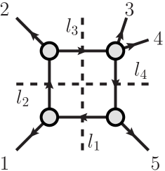
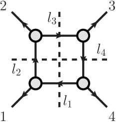
Refer to caption

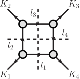
Figure 1: A general quadruple cut. Loop momenta flow clockwise.

For the quadruple cut (Fig. 1) in 42ϵ42italic-ϵ4-2\epsilon dimensions, the on-shell cut conditions are

l12=l22=l32=l42=0,superscriptsubscript𝑙12superscriptsubscript𝑙22superscriptsubscript𝑙32superscriptsubscript𝑙420\displaystyle l_{1}^{2}=l_{2}^{2}=l_{3}^{2}=l_{4}^{2}=0, (31)

or equivalently,

l¯12=l¯22=l¯32=l¯42=μ2,superscriptsubscript¯𝑙12superscriptsubscript¯𝑙22superscriptsubscript¯𝑙32superscriptsubscript¯𝑙42superscript𝜇2\displaystyle\bar{l}_{1}^{2}=\bar{l}_{2}^{2}=\bar{l}_{3}^{2}=\bar{l}_{4}^{2}=\mu^{2}, (32)

where l¯isubscript¯𝑙𝑖\bar{l}_{i} are the momenta truncated to four dimensions and μ𝜇\mu represents the (2ϵ)2italic-ϵ(-2\epsilon)-dimensional components. It is convenient to view μ2superscript𝜇2\mu^{2} as a mass term and the internal momenta as four-dimensionally massive. (This is the view taken in ref. Badger and as we saw a useful one for six-dimensional helicity as well.) We parametrize the four-momentum l¯1subscript¯𝑙1\bar{l}_{1} using a construction first given in refs. OPP1 ; OPP2 ; AguilaPittau and also applied in refs. Forde ; Badger ; Kilgore ,

l¯1μ=12(aK4|γμ|K4+bK1|γμ|K1+cK4|γμ|K1+dK1|γμ|K4),superscriptsubscript¯𝑙1𝜇12𝑎quantum-operator-productsuperscriptsubscript𝐾4limit-fromsuperscript𝛾𝜇superscriptsubscript𝐾4limit-from𝑏quantum-operator-productsuperscriptsubscript𝐾1limit-fromsuperscript𝛾𝜇superscriptsubscript𝐾1limit-from𝑐quantum-operator-productsuperscriptsubscript𝐾4limit-fromsuperscript𝛾𝜇superscriptsubscript𝐾1limit-from𝑑quantum-operator-productsuperscriptsubscript𝐾1limit-fromsuperscript𝛾𝜇superscriptsubscript𝐾4limit-from\displaystyle\bar{l}_{1}^{\mu}=\frac{1}{2}(a\langle K_{4}^{\flat-}|\gamma^{\mu}|K_{4}^{\flat-}\rangle+b\langle K_{1}^{\flat-}|\gamma^{\mu}|K_{1}^{\flat-}\rangle+c\langle K_{4}^{\flat-}|\gamma^{\mu}|K_{1}^{\flat-}\rangle+d\langle K_{1}^{\flat-}|\gamma^{\mu}|K_{4}^{\flat-}\rangle), (33)

where K1,4superscriptsubscript𝐾14K_{1,4}^{\flat} is the massless projection of one of the external legs in the direction of the other masslessly projected leg,

K1μ=γ14(γ14K1μS1K4μ)γ142S1S4,K4μ=γ14(γ14K4μS4K1μ)γ142S1S4,formulae-sequencesuperscriptsubscript𝐾1𝜇subscript𝛾14subscript𝛾14superscriptsubscript𝐾1𝜇subscript𝑆1superscriptsubscript𝐾4𝜇superscriptsubscript𝛾142subscript𝑆1subscript𝑆4superscriptsubscript𝐾4𝜇subscript𝛾14subscript𝛾14superscriptsubscript𝐾4𝜇subscript𝑆4superscriptsubscript𝐾1𝜇superscriptsubscript𝛾142subscript𝑆1subscript𝑆4\displaystyle K_{1}^{\flat\mu}=\frac{\gamma_{14}(\gamma_{14}K_{1}^{\mu}-S_{1}K_{4}^{\mu})}{\gamma_{14}^{2}-S_{1}S_{4}},\hskip 28.45274ptK_{4}^{\flat\mu}=\frac{\gamma_{14}(\gamma_{14}K_{4}^{\mu}-S_{4}K_{1}^{\mu})}{\gamma_{14}^{2}-S_{1}S_{4}},
γ14=K1K4±(K1K4)2S1S4,Si=Ki2.formulae-sequencesubscript𝛾14plus-or-minussubscript𝐾1subscript𝐾4superscriptsubscript𝐾1subscript𝐾42subscript𝑆1subscript𝑆4subscript𝑆𝑖superscriptsubscript𝐾𝑖2\displaystyle\gamma_{14}=K_{1}\cdot K_{4}\pm\sqrt{(K_{1}\cdot K_{4})^{2}-S_{1}S_{4}},\hskip 28.45274ptS_{i}=K_{i}^{2}. (34)

Solving the on-shell conditions, we find that l¯1subscript¯𝑙1\bar{l}_{1} can be expanded as

l¯1μsuperscriptsubscript¯𝑙1𝜇\displaystyle\bar{l}_{1}^{\mu} =aK4μ+bK1μ+c±2K4|γμ|K1+γ14abμ22c±γ14K1|γμ|K4absent𝑎superscriptsubscript𝐾4𝜇𝑏superscriptsubscript𝐾1𝜇subscript𝑐plus-or-minus2quantum-operator-productsuperscriptsubscript𝐾4limit-fromsuperscript𝛾𝜇superscriptsubscript𝐾1limit-fromsubscript𝛾14𝑎𝑏superscript𝜇22subscript𝑐plus-or-minussubscript𝛾14quantum-operator-productsuperscriptsubscript𝐾1limit-fromsuperscript𝛾𝜇superscriptsubscript𝐾4limit-from\displaystyle=aK_{4}^{\flat\mu}+bK_{1}^{\flat\mu}+\frac{c_{\pm}}{2}\langle K_{4}^{\flat-}|\gamma^{\mu}|K_{1}^{\flat-}\rangle+\frac{\gamma_{14}ab-\mu^{2}}{2c_{\pm}\gamma_{14}}\langle K_{1}^{\flat-}|\gamma^{\mu}|K_{4}^{\flat-}\rangle
=l¯1μμ22c±γ14K1|γμ|K4,absentsuperscriptsubscript¯𝑙1𝜇superscript𝜇22subscript𝑐plus-or-minussubscript𝛾14quantum-operator-productsuperscriptsubscript𝐾1limit-fromsuperscript𝛾𝜇superscriptsubscript𝐾4limit-from\displaystyle=\bar{l}_{1}^{\flat\mu}-\frac{\mu^{2}}{2c_{\pm}\gamma_{14}}\langle K_{1}^{\flat-}|\gamma^{\mu}|K_{4}^{\flat-}\rangle, (35)

where

a=S1(S4+γ14)γ142S1S4,b=S4(S1+γ14)γ142S1S4,c±=c1±c124c0c22c2,formulae-sequence𝑎subscript𝑆1subscript𝑆4subscript𝛾14superscriptsubscript𝛾142subscript𝑆1subscript𝑆4formulae-sequence𝑏subscript𝑆4subscript𝑆1subscript𝛾14superscriptsubscript𝛾142subscript𝑆1subscript𝑆4subscript𝑐plus-or-minusplus-or-minussubscript𝑐1superscriptsubscript𝑐124subscript𝑐0subscript𝑐22subscript𝑐2\displaystyle a=\frac{S_{1}(S_{4}+\gamma_{14})}{\gamma_{14}^{2}-S_{1}S_{4}},\hskip 17.07164ptb=-\frac{S_{4}(S_{1}+\gamma_{14})}{\gamma_{14}^{2}-S_{1}S_{4}},\hskip 17.07164ptc_{\pm}=\frac{-c_{1}\pm\sqrt{c_{1}^{2}-4c_{0}c_{2}}}{2c_{2}},
c2subscript𝑐2\displaystyle c_{2} =K4|/K2|K1,absentquantum-operator-productsuperscriptsubscript𝐾4limit-fromsubscript/K2superscriptsubscript𝐾1limit-from\displaystyle=\langle K_{4}^{\flat-}|{\raise 0.91666pt\hbox to9.20833pt{\hss/\hss}\hbox to0.0pt{\hss$K$}}_{2}|K_{1}^{\flat-}\rangle,
c1subscript𝑐1\displaystyle c_{1} =aK4|/K2|K4+bK1|/K2|K1S22K1K2,absent𝑎quantum-operator-productsuperscriptsubscript𝐾4limit-fromsubscript/K2superscriptsubscript𝐾4limit-from𝑏quantum-operator-productsuperscriptsubscript𝐾1limit-fromsubscript/K2superscriptsubscript𝐾1limit-fromsubscript𝑆22subscript𝐾1subscript𝐾2\displaystyle=a\langle K_{4}^{\flat-}|{\raise 0.91666pt\hbox to9.20833pt{\hss/\hss}\hbox to0.0pt{\hss$K$}}_{2}|K_{4}^{\flat-}\rangle+b\langle K_{1}^{\flat-}|{\raise 0.91666pt\hbox to9.20833pt{\hss/\hss}\hbox to0.0pt{\hss$K$}}_{2}|K_{1}^{\flat-}\rangle-S_{2}-2K_{1}\cdot K_{2},
c0subscript𝑐0\displaystyle c_{0} =(abμ2γ14)K1|/K2|K4.absent𝑎𝑏superscript𝜇2subscript𝛾14quantum-operator-productsuperscriptsubscript𝐾1limit-fromsubscript/K2superscriptsubscript𝐾4limit-from\displaystyle=\left(ab-\frac{\mu^{2}}{\gamma_{14}}\right)\langle K_{1}^{\flat-}|{\raise 0.91666pt\hbox to9.20833pt{\hss/\hss}\hbox to0.0pt{\hss$K$}}_{2}|K_{4}^{\flat-}\rangle. (36)

In general there are two solutions to the on-shell conditions. It would appear initially that there are four, two each for γ14subscript𝛾14\gamma_{14} and c±subscript𝑐plus-or-minusc_{\pm}, but it turns out that,

l¯1(γ14+,c+)subscript¯𝑙1superscriptsubscript𝛾14subscript𝑐\displaystyle\bar{l}_{1}(\gamma_{14}^{+},c_{+}) =l¯1(γ14,c),absentsubscript¯𝑙1superscriptsubscript𝛾14subscript𝑐\displaystyle=\bar{l}_{1}(\gamma_{14}^{-},c_{-}),
l¯1(γ14+,c)subscript¯𝑙1superscriptsubscript𝛾14subscript𝑐\displaystyle\bar{l}_{1}(\gamma_{14}^{+},c_{-}) =l¯1(γ14,c+).absentsubscript¯𝑙1superscriptsubscript𝛾14subscript𝑐\displaystyle=\bar{l}_{1}(\gamma_{14}^{-},c_{+}). (37)

In the case S1=0subscript𝑆10S_{1}=0 or S4=0subscript𝑆40S_{4}=0, there is only one solution for γ14subscript𝛾14\gamma_{14} (but still two solutions to the on-shell conditions). To determine the full box coefficient, we must average over these solutions.

Using these solutions to define spinors, we can calculate the four tree amplitudes associated with the quadruple cut. As explained in Appendix B, the coefficients associated with our integral basis choice (29) are

C4[0]superscriptsubscript𝐶4delimited-[]0\displaystyle C_{4}^{[0]} =i2σA1A2A3A4(l¯1σ)|μ20,absentevaluated-at𝑖2subscript𝜎subscript𝐴1subscript𝐴2subscript𝐴3subscript𝐴4superscriptsubscript¯𝑙1𝜎superscript𝜇20\displaystyle=\frac{i}{2}\sum_{\sigma}\left.A_{1}A_{2}A_{3}A_{4}(\bar{l}_{1}^{\sigma})\right|_{\mu^{2}\rightarrow 0},
C4[4]superscriptsubscript𝐶4delimited-[]4\displaystyle C_{4}^{[4]} =i2σ[Infμ2A1A2A3A4](μ2)|μ4.absentevaluated-at𝑖2subscript𝜎delimited-[]subscriptInfsuperscript𝜇2subscript𝐴1subscript𝐴2subscript𝐴3subscript𝐴4superscript𝜇2superscript𝜇4\displaystyle=\frac{i}{2}\sum_{\sigma}\left.[\mathrm{Inf}_{\mu^{2}}A_{1}A_{2}A_{3}A_{4}](\mu^{2})\right|_{\mu^{4}}. (38)

The sum is over the two solutions to the quadruple cut; the product A1A2A3A4subscript𝐴1subscript𝐴2subscript𝐴3subscript𝐴4A_{1}A_{2}A_{3}A_{4} must be computed for each. To find C4[0]superscriptsubscript𝐶4delimited-[]0C_{4}^{[0]}, our cut-constructible piece, we set μ2=0superscript𝜇20\mu^{2}=0. The Inf term in C4[4]superscriptsubscript𝐶4delimited-[]4C_{4}^{[4]}, first given in ref. BernInf , contains the information from the boundary of the μ𝜇\mu contour integral,

limμ([Infμ2A1A2A3A4](μ2)A1(μ)A2(μ)A3(μ)A4(μ))=0.subscript𝜇delimited-[]subscriptInfsuperscript𝜇2subscript𝐴1subscript𝐴2subscript𝐴3subscript𝐴4superscript𝜇2subscript𝐴1𝜇subscript𝐴2𝜇subscript𝐴3𝜇subscript𝐴4𝜇0\displaystyle\lim_{\mu\rightarrow\infty}([\mathrm{Inf}_{\mu^{2}}A_{1}A_{2}A_{3}A_{4}](\mu^{2})-A_{1}(\mu)A_{2}(\mu)A_{3}(\mu)A_{4}(\mu))=0. (39)

We expand around infinity and write it as a polynomial in μ2superscript𝜇2\mu^{2},

[Infμ2A1A2A3A4](μ2)=i=02ciμ2i,delimited-[]subscriptInfsuperscript𝜇2subscript𝐴1subscript𝐴2subscript𝐴3subscript𝐴4superscript𝜇2superscriptsubscript𝑖02subscript𝑐𝑖superscript𝜇2𝑖\displaystyle[\mathrm{Inf}_{\mu^{2}}A_{1}A_{2}A_{3}A_{4}](\mu^{2})=\sum_{i=0}^{2}c_{i}\mu^{2i}, (40)

then restrict C4[4]superscriptsubscript𝐶4delimited-[]4C_{4}^{[4]} to be the coefficient of the μ4superscript𝜇4\mu^{4} term, explaining the notation of eq. (38).

IV.2 Triangle integral coefficients

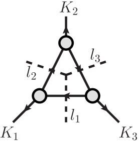
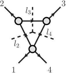
Refer to caption

Figure 2: A general triple cut.

To obtain the solution to the triple cut (Fig. 2), we again parametrize our loop momentum in terms of adjacent projected external momenta,

l¯1μsuperscriptsubscript¯𝑙1𝜇\displaystyle\bar{l}_{1}^{\mu} =aK3μ+bK1μ+t2K3|γμ|K1+γ13abμ22tγ13K1|γμ|K3,absent𝑎superscriptsubscript𝐾3𝜇𝑏superscriptsubscript𝐾1𝜇𝑡2quantum-operator-productsuperscriptsubscript𝐾3limit-fromsuperscript𝛾𝜇superscriptsubscript𝐾1limit-fromsubscript𝛾13𝑎𝑏superscript𝜇22𝑡subscript𝛾13quantum-operator-productsuperscriptsubscript𝐾1limit-fromsuperscript𝛾𝜇superscriptsubscript𝐾3limit-from\displaystyle=aK_{3}^{\flat\mu}+bK_{1}^{\flat\mu}+\frac{t}{2}\langle K_{3}^{\flat-}|\gamma^{\mu}|K_{1}^{\flat-}\rangle+\frac{\gamma_{13}ab-\mu^{2}}{2t\gamma_{13}}\langle K_{1}^{\flat-}|\gamma^{\mu}|K_{3}^{\flat-}\rangle, (41)

where K1superscriptsubscript𝐾1K_{1}^{\flat} and K3superscriptsubscript𝐾3K_{3}^{\flat} are defined analogously to eq. (IV.1). The coefficients a𝑎a and b𝑏b are defined in eq. (IV.1) and γ13subscript𝛾13\gamma_{13} is defined in eq. (IV.1) (with K3superscriptsubscript𝐾3K_{3}^{\flat} replacing K4superscriptsubscript𝐾4K_{4}^{\flat} in both). We must average over the solutions for γ13subscript𝛾13\gamma_{13}, though in the case that S1=0subscript𝑆10S_{1}=0 or S3=0subscript𝑆30S_{3}=0, there is only one solution. For a fixed value of γ13subscript𝛾13\gamma_{13}, we must also average over the coefficients given by the conjugate solution,

l¯1μsuperscriptsubscript¯𝑙1absent𝜇\displaystyle\bar{l}_{1}^{*\mu} =aK3μ+bK1μ+t2K1|γμ|K3+γ13abμ22tγ13K3|γμ|K1.absent𝑎superscriptsubscript𝐾3𝜇𝑏superscriptsubscript𝐾1𝜇𝑡2quantum-operator-productsuperscriptsubscript𝐾1limit-fromsuperscript𝛾𝜇superscriptsubscript𝐾3limit-fromsubscript𝛾13𝑎𝑏superscript𝜇22𝑡subscript𝛾13quantum-operator-productsuperscriptsubscript𝐾3limit-fromsuperscript𝛾𝜇superscriptsubscript𝐾1limit-from\displaystyle=aK_{3}^{\flat\mu}+bK_{1}^{\flat\mu}+\frac{t}{2}\langle K_{1}^{\flat-}|\gamma^{\mu}|K_{3}^{\flat-}\rangle+\frac{\gamma_{13}ab-\mu^{2}}{2t\gamma_{13}}\langle K_{3}^{\flat-}|\gamma^{\mu}|K_{1}^{\flat-}\rangle. (42)

In both solutions the complex parameter t𝑡t is free.

Box integrals also contain triple cuts, so we must extract the triangle coefficients using the limiting behavior of the integrand. The coefficients therefore contain an Inf term that is a polynomial expansion in t𝑡t,

C3[0]superscriptsubscript𝐶3delimited-[]0\displaystyle C_{3}^{[0]} =12nγσ[InftA1A2A3(l¯1σ)](t)|μ20,t0,absentevaluated-at12subscript𝑛𝛾subscript𝜎delimited-[]subscriptInf𝑡subscript𝐴1subscript𝐴2subscript𝐴3superscriptsubscript¯𝑙1𝜎𝑡formulae-sequencesuperscript𝜇20𝑡0\displaystyle=-\frac{1}{2n_{\gamma}}\sum_{\sigma}\left.[\mathrm{Inf}_{t}A_{1}A_{2}A_{3}(\bar{l}_{1}^{\sigma})](t)\right|_{\mu^{2}\rightarrow 0,t\rightarrow 0},
C3[2]superscriptsubscript𝐶3delimited-[]2\displaystyle C_{3}^{[2]} =12nγσ[Infμ2[InftA1A2A3(l¯1σ)](t)](μ2)|μ2,t0,absentevaluated-at12subscript𝑛𝛾subscript𝜎delimited-[]subscriptInfsuperscript𝜇2delimited-[]subscriptInf𝑡subscript𝐴1subscript𝐴2subscript𝐴3superscriptsubscript¯𝑙1𝜎𝑡superscript𝜇2superscript𝜇2𝑡0\displaystyle=-\frac{1}{2n_{\gamma}}\sum_{\sigma}\left.[\mathrm{Inf}_{\mu^{2}}[\mathrm{Inf}_{t}A_{1}A_{2}A_{3}(\bar{l}_{1}^{\sigma})](t)](\mu^{2})\right|_{\mu^{2},t\rightarrow 0}, (43)

but only the order t0superscript𝑡0t^{0} term is retained. The sum is over the solutions, including the conjugate-momentum solution, to the cut conditions. There may be either two or four solutions depending on the number of solutions nγsubscript𝑛𝛾n_{\gamma} for γ13subscript𝛾13\gamma_{13}. In C3[0]superscriptsubscript𝐶3delimited-[]0C_{3}^{[0]}, μ2superscript𝜇2\mu^{2} and t𝑡t are both set to zero, while the expansion in C3[2]superscriptsubscript𝐶3delimited-[]2C_{3}^{[2]} is restricted to the coefficients of the μ2superscript𝜇2\mu^{2} term (in addition to having t=0𝑡0t=0).

IV.3 Bubble integral coefficients

Refer to caption
(a)
Refer to caption
(b)
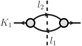
Figure 3: Double and triple cuts contributing to bubble coefficients.

Two-particle cuts are contaminated by both boxes and triangles, so again an extraction procedure is necessary. Furthermore, triple cuts that share two of their cuts with the double cut contribute to tensor triangle integrals that reduce to scalar bubbles, so we must take them into account for the full bubble coefficient (Fig. 3). The two-particle cut momentum solution has two free parameters t𝑡t and y𝑦y,

l¯1μ=yK1μ+S1(1y)γ¯χμ+t2K1|γμ|χ+y(1y)S1μ22tγ¯χ|γμ|K1,superscriptsubscript¯𝑙1𝜇𝑦superscriptsubscript𝐾1𝜇subscript𝑆11𝑦¯𝛾superscript𝜒𝜇𝑡2quantum-operator-productsuperscriptsubscript𝐾1limit-fromsuperscript𝛾𝜇superscript𝜒𝑦1𝑦subscript𝑆1superscript𝜇22𝑡¯𝛾quantum-operator-productsuperscript𝜒superscript𝛾𝜇superscriptsubscript𝐾1limit-from\displaystyle\bar{l}_{1}^{\mu}=yK_{1}^{\flat\mu}+\frac{S_{1}(1-y)}{\bar{\gamma}}\chi^{\mu}+\frac{t}{2}\langle K_{1}^{\flat-}|\gamma^{\mu}|\chi^{-}\rangle+\frac{y(1-y)S_{1}-\mu^{2}}{2t\bar{\gamma}}\langle\chi^{-}|\gamma^{\mu}|K_{1}^{\flat-}\rangle, (44)

where

K1μ=K1μS1γ¯χμ,γ¯=2(K1χ),formulae-sequencesuperscriptsubscript𝐾1𝜇superscriptsubscript𝐾1𝜇subscript𝑆1¯𝛾superscript𝜒𝜇¯𝛾2subscript𝐾1𝜒\displaystyle K_{1}^{\flat\mu}=K_{1}^{\mu}-\frac{S_{1}}{\bar{\gamma}}\chi^{\mu},\hskip 28.45274pt\bar{\gamma}=2(K_{1}\cdot\chi), (45)

and χ𝜒\chi is some arbitrary massless vector. We calculate the cut integrand A1A2subscript𝐴1subscript𝐴2A_{1}A_{2} by taking a product of the two on-shell tree amplitudes, which will make up part of our coefficient after an extraction procedure.

For the triangle contribution to the bubble coefficient, we fix the parameter y𝑦y to put another propagator on shell,

y±=B1±B12+4B0B22B2,subscript𝑦plus-or-minusplus-or-minussubscript𝐵1superscriptsubscript𝐵124subscript𝐵0subscript𝐵22subscript𝐵2\displaystyle y_{\pm}=\frac{B_{1}\pm\sqrt{B_{1}^{2}+4B_{0}B_{2}}}{2B_{2}}, (46)

where

B2subscript𝐵2\displaystyle B_{2} =S1χ|/K3|K1,absentsubscript𝑆1quantum-operator-productsuperscript𝜒subscript/K3superscriptsubscript𝐾1limit-from\displaystyle=S_{1}\langle\chi^{-}|{\raise 0.91666pt\hbox to9.20833pt{\hss/\hss}\hbox to0.0pt{\hss$K$}}_{3}|K_{1}^{\flat-}\rangle,
B1subscript𝐵1\displaystyle B_{1} =γ¯tK1|/K3|K1S1tχ|/K3|χ+S1χ|/K3|K1,absent¯𝛾𝑡quantum-operator-productsuperscriptsubscript𝐾1limit-fromsubscript/K3superscriptsubscript𝐾1limit-fromsubscript𝑆1𝑡quantum-operator-productsuperscript𝜒subscript/K3superscript𝜒subscript𝑆1quantum-operator-productsuperscript𝜒subscript/K3superscriptsubscript𝐾1limit-from\displaystyle=\bar{\gamma}t\langle K_{1}^{\flat-}|{\raise 0.91666pt\hbox to9.20833pt{\hss/\hss}\hbox to0.0pt{\hss$K$}}_{3}|K_{1}^{\flat-}\rangle-S_{1}t\langle\chi^{-}|{\raise 0.91666pt\hbox to9.20833pt{\hss/\hss}\hbox to0.0pt{\hss$K$}}_{3}|\chi^{-}\rangle+S_{1}\langle\chi^{-}|{\raise 0.91666pt\hbox to9.20833pt{\hss/\hss}\hbox to0.0pt{\hss$K$}}_{3}|K_{1}^{\flat-}\rangle,
B0subscript𝐵0\displaystyle B_{0} =γ¯t2K1|/K3|χμ2χ|/K3|K1+γ¯tS3+tS1χ|/K3|χ.absent¯𝛾superscript𝑡2quantum-operator-productsuperscriptsubscript𝐾1limit-fromsubscript/K3superscript𝜒superscript𝜇2quantum-operator-productsuperscript𝜒subscript/K3superscriptsubscript𝐾1limit-from¯𝛾𝑡subscript𝑆3𝑡subscript𝑆1quantum-operator-productsuperscript𝜒subscript/K3superscript𝜒\displaystyle=\bar{\gamma}t^{2}\langle K_{1}^{\flat-}|{\raise 0.91666pt\hbox to9.20833pt{\hss/\hss}\hbox to0.0pt{\hss$K$}}_{3}|\chi^{-}\rangle-\mu^{2}\langle\chi^{-}|{\raise 0.91666pt\hbox to9.20833pt{\hss/\hss}\hbox to0.0pt{\hss$K$}}_{3}|K_{1}^{\flat-}\rangle+\bar{\gamma}tS_{3}+tS_{1}\langle\chi^{-}|{\raise 0.91666pt\hbox to9.20833pt{\hss/\hss}\hbox to0.0pt{\hss$K$}}_{3}|\chi^{-}\rangle. (47)

We then calculate the triple-cut integrand A1A2A3subscript𝐴1subscript𝐴2subscript𝐴3A_{1}A_{2}A_{3} for all triple cuts that share two cuts with the original double cut. The bubble coefficients are then given by

C2[0]=superscriptsubscript𝐶2delimited-[]0absent\displaystyle C_{2}^{[0]}= i[Inft[InfyA1A2](y)](t)|μ20,t0,ymYm12Ctriσy[InftA1A2A3](t)|μ20,tjTj,evaluated-at𝑖delimited-[]subscriptInf𝑡delimited-[]subscriptInf𝑦subscript𝐴1subscript𝐴2𝑦𝑡formulae-sequencesuperscript𝜇20formulae-sequence𝑡0superscript𝑦𝑚subscript𝑌𝑚evaluated-at12subscriptsubscript𝐶trisubscriptsubscript𝜎𝑦delimited-[]subscriptInf𝑡subscript𝐴1subscript𝐴2subscript𝐴3𝑡formulae-sequencesuperscript𝜇20superscript𝑡𝑗subscript𝑇𝑗\displaystyle-i[\mathrm{Inf}_{t}[\mathrm{Inf}_{y}A_{1}A_{2}](y)](t)|_{\mu^{2}\rightarrow 0,t\rightarrow 0,y^{m}\rightarrow Y_{m}}-\frac{1}{2}\sum_{C_{\mathrm{tri}}}\sum_{\sigma_{y}}[\mathrm{Inf}_{t}A_{1}A_{2}A_{3}](t)|_{\mu^{2}\rightarrow 0,t^{j}\rightarrow T_{j}},
C2[2]=superscriptsubscript𝐶2delimited-[]2absent\displaystyle C_{2}^{[2]}= i[Infμ2[Inft[InfyA1A2](y)](t)](μ2)|μ2,t0,ymYmevaluated-at𝑖delimited-[]subscriptInfsuperscript𝜇2delimited-[]subscriptInf𝑡delimited-[]subscriptInf𝑦subscript𝐴1subscript𝐴2𝑦𝑡superscript𝜇2formulae-sequencesuperscript𝜇2𝑡0superscript𝑦𝑚subscript𝑌𝑚\displaystyle-i[\mathrm{Inf}_{\mu^{2}}[\mathrm{Inf}_{t}[\mathrm{Inf}_{y}A_{1}A_{2}](y)](t)](\mu^{2})|_{\mu^{2},t\rightarrow 0,y^{m}\rightarrow Y_{m}}
12Ctriσy[Infμ2[InftA1A2A3](t)](μ2)|μ2,tjTj.evaluated-at12subscriptsubscript𝐶trisubscriptsubscript𝜎𝑦delimited-[]subscriptInfsuperscript𝜇2delimited-[]subscriptInf𝑡subscript𝐴1subscript𝐴2subscript𝐴3𝑡superscript𝜇2superscript𝜇2superscript𝑡𝑗subscript𝑇𝑗\displaystyle-\frac{1}{2}\sum_{C_{\mathrm{tri}}}\sum_{\sigma_{y}}[\mathrm{Inf}_{\mu^{2}}[\mathrm{Inf}_{t}A_{1}A_{2}A_{3}](t)](\mu^{2})|_{\mu^{2},t^{j}\rightarrow T_{j}}. (48)

In the series expansion [InfyA1A2](y)=m=0kfmymdelimited-[]subscriptInf𝑦subscript𝐴1subscript𝐴2𝑦superscriptsubscript𝑚0𝑘subscript𝑓𝑚superscript𝑦𝑚[\mathrm{Inf}_{y}A_{1}A_{2}](y)=\sum_{m=0}^{k}f_{m}y^{m}, we make the replacements ymYmsuperscript𝑦𝑚subscript𝑌𝑚y^{m}\rightarrow Y_{m} where

Y0=1,Y1=12,Y2=13(1μ2S1),Y3=14(12μ2S1),Y4=15(13μ2S1+μ4S12).formulae-sequencesubscript𝑌01formulae-sequencesubscript𝑌112formulae-sequencesubscript𝑌2131superscript𝜇2subscript𝑆1formulae-sequencesubscript𝑌31412superscript𝜇2subscript𝑆1subscript𝑌41513superscript𝜇2subscript𝑆1superscript𝜇4superscriptsubscript𝑆12\displaystyle Y_{0}=1,\hskip 11.38109ptY_{1}=\frac{1}{2},\hskip 11.38109ptY_{2}=\frac{1}{3}\left(1-\frac{\mu^{2}}{S_{1}}\right),\hskip 11.38109ptY_{3}=\frac{1}{4}\left(1-2\frac{\mu^{2}}{S_{1}}\right),\hskip 11.38109ptY_{4}=\frac{1}{5}\left(1-3\frac{\mu^{2}}{S_{1}}+\frac{\mu^{4}}{S_{1}^{2}}\right). (49)

These double-cut terms are also expanded in t𝑡t and restricted to the t0superscript𝑡0t^{0} term. In C2[0]superscriptsubscript𝐶2delimited-[]0C_{2}^{[0]}, μ2superscript𝜇2\mu^{2} is set to zero, while in C2[2]superscriptsubscript𝐶2delimited-[]2C_{2}^{[2]} there is an expansion in μ2superscript𝜇2\mu^{2}, and C2[2]superscriptsubscript𝐶2delimited-[]2C_{2}^{[2]} is restricted to the order μ2superscript𝜇2\mu^{2} coefficient. The triple-cut terms have a sum over the two solutions for each triple cut and a sum over all possible triple cuts that share two cuts with the double cut. In the expansion in t𝑡t, we replace tjTjsuperscript𝑡𝑗subscript𝑇𝑗t^{j}\rightarrow T_{j} where

T0subscript𝑇0\displaystyle T_{0} =0,absent0\displaystyle=0,
T1subscript𝑇1\displaystyle T_{1} =S1χ|/K3|K12γ¯Δ,absentsubscript𝑆1quantum-operator-productsuperscript𝜒subscript/K3superscriptsubscript𝐾1limit-from2¯𝛾Δ\displaystyle=-\frac{S_{1}\langle\chi^{-}|{\raise 0.91666pt\hbox to9.20833pt{\hss/\hss}\hbox to0.0pt{\hss$K$}}_{3}|K_{1}^{\flat-}\rangle}{2\bar{\gamma}\Delta},
T2subscript𝑇2\displaystyle T_{2} =3S1χ|/K3|K128γ¯2Δ2(S1S3+K1K3S1),absent3subscript𝑆1superscriptquantum-operator-productsuperscript𝜒subscript/K3superscriptsubscript𝐾1limit-from28superscript¯𝛾2superscriptΔ2subscript𝑆1subscript𝑆3subscript𝐾1subscript𝐾3subscript𝑆1\displaystyle=-\frac{3S_{1}\langle\chi^{-}|{\raise 0.91666pt\hbox to9.20833pt{\hss/\hss}\hbox to0.0pt{\hss$K$}}_{3}|K_{1}^{\flat-}\rangle^{2}}{8\bar{\gamma}^{2}\Delta^{2}}(S_{1}S_{3}+K_{1}\cdot K_{3}S_{1}),
T3subscript𝑇3\displaystyle T_{3} =χ|/K3|K1348γ¯3Δ3(15S13S32+30K1K3S13S3+11(K1K3)2S13+4S14S3+16μ2S12Δ),absentsuperscriptquantum-operator-productsuperscript𝜒subscript/K3superscriptsubscript𝐾1limit-from348superscript¯𝛾3superscriptΔ315superscriptsubscript𝑆13superscriptsubscript𝑆3230subscript𝐾1subscript𝐾3superscriptsubscript𝑆13subscript𝑆311superscriptsubscript𝐾1subscript𝐾32superscriptsubscript𝑆134superscriptsubscript𝑆14subscript𝑆316superscript𝜇2superscriptsubscript𝑆12Δ\displaystyle=-\frac{\langle\chi^{-}|{\raise 0.91666pt\hbox to9.20833pt{\hss/\hss}\hbox to0.0pt{\hss$K$}}_{3}|K_{1}^{\flat-}\rangle^{3}}{48\bar{\gamma}^{3}\Delta^{3}}\left(15S_{1}^{3}S_{3}^{2}+30K_{1}\cdot K_{3}S_{1}^{3}S_{3}+11(K_{1}\cdot K_{3})^{2}S_{1}^{3}+4S_{1}^{4}S_{3}+16\mu^{2}S_{1}^{2}\Delta\right), (50)

and

Δ=(K1K3)2S1S3.Δsuperscriptsubscript𝐾1subscript𝐾32subscript𝑆1subscript𝑆3\displaystyle\Delta=(K_{1}\cdot K_{3})^{2}-S_{1}S_{3}. (51)

In a renormalizable gauge theory (such as QCD), double cuts can have terms up to order y4superscript𝑦4y^{4} while triple cuts can have up to t3superscript𝑡3t^{3}, so all necessary integrals are evaluated above.111As it turns out, y3superscript𝑦3y^{3} and y4superscript𝑦4y^{4} terms come with factors of 1/t1𝑡1/t and 1/t21superscript𝑡21/t^{2}, respectively, so such terms drop out when the coefficient is restricted to the t0superscript𝑡0t^{0} term, but we include the evaluations above so as not to break the procedural nature of the method. Again see Appendix B for a more detailed explanation.

V COMPUTATION OF FOUR- AND FIVE-POINT GLUON AMPLITUDES

With the formalism established, we turn to sample calculations of one-loop amplitudes in QCD, starting with A4(1)(1,2+,3+,4+)superscriptsubscript𝐴41superscript1superscript2superscript3superscript4A_{4}^{(1)}(1^{-},2^{+},3^{+},4^{+}) for a scalar loop, gluon loop and fermion loop. We use generalized unitarity to glue together tree amplitudes written in terms of six-dimensional spinors. In keeping with Cheung and O’Connell COC6D , these six-dimensional spinors are written in terms of four-dimensional ones based on the loop-momentum solutions of section IV. The cuts then fall into a form that allows us to use our coefficient extraction techniques. Our methodology for the cuts follows that of ref. Bern6D .

As mentioned earlier, internal particles are kept in six dimensions while external particles live in the four-dimensional subspace. This leads to an additional complication: increasing the number of spacetime dimensions also increases the number of spin eigenstates. We therefore do not expect the six-dimensional coefficients to exactly match the four-dimensional ones, and in fact we must perform a state-sum reduction to bring our result back to four dimensions.

We find that the scalar-loop diagram does not require adjustment, nor does the fermion loop. For the gluon-loop diagram, however, we must subtract two factors of the scalar-loop diagram. We motivate these procedures by tracking how the dimension makes its way into the integral coefficients and demonstrate their effectiveness in the one-loop amplitude A4(1)(1,2+,3+,4+)superscriptsubscript𝐴41superscript1superscript2superscript3superscript4A_{4}^{(1)}(1^{-},2^{+},3^{+},4^{+}). We then include some additional results, but with fewer computational details.

V.1 One-loop four-point cut conditions in D=6𝐷6D=6
Refer to caption
(a)
Refer to caption
(b)
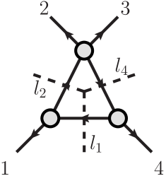
Refer to caption
(c)
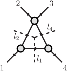
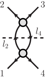
Figure 4: Cuts for the four-point amplitude. We show triple and double cuts in the s23subscript𝑠23s_{23} channel; in general we must also evaluate cuts in the s12subscript𝑠12s_{12} channel.

To compute the amplitudes using six-dimensional helicity, we use momentum solutions from section IV that fit with the coefficient extraction techniques. There we interpreted the (2ϵ)2italic-ϵ(-2\epsilon)-dimensional component μ𝜇\mu as a mass and gave the four-dimensional components of the loop momenta the on-shell cut conditions, l¯i2=μ2superscriptsubscript¯𝑙𝑖2superscript𝜇2\bar{l}_{i}^{2}=\mu^{2}. In section II we also expressed the extra-dimensional components of six-dimensional momenta in terms of mass parameters m𝑚m and m~~𝑚\tilde{m} given in eq. (12),

li4=m+m~2i,li5=m+m~2,formulae-sequencesuperscriptsubscript𝑙𝑖4𝑚~𝑚2𝑖superscriptsubscript𝑙𝑖5𝑚~𝑚2\displaystyle l_{i}^{4}=\frac{-m+\tilde{m}}{2i},\hskip 85.35826ptl_{i}^{5}=\frac{m+\tilde{m}}{2}, (52)

giving the on-shell cut conditions, l¯i2=mm~superscriptsubscript¯𝑙𝑖2𝑚~𝑚\bar{l}_{i}^{2}=m\tilde{m}. This enabled us to embed four-dimensional spinors in the six-dimensional ones. Making the association μ2mm~superscript𝜇2𝑚~𝑚\mu^{2}\leftrightarrow m\tilde{m}, we see that we have a bi-spinor momentum representation that simultaneously allows us to use six-dimensional helicity and the coefficient extraction techniques.

Using eq. (35), the momentum solution for the quadruple cut (Fig. 4a) is

(l¯±)1μ=12(c1±4|γμ|11c1±mm~s141|γμ|4),superscriptsubscriptsuperscript¯𝑙plus-or-minus1𝜇12superscriptsubscript𝑐1plus-or-minusquantum-operator-productsuperscript4superscript𝛾𝜇superscript11superscriptsubscript𝑐1plus-or-minus𝑚~𝑚subscript𝑠14quantum-operator-productsuperscript1superscript𝛾𝜇superscript4(\bar{l}^{\pm})_{1}^{\mu}=\frac{1}{2}\left(c_{1}^{\pm}\langle 4^{-}|\gamma^{\mu}|1^{-}\rangle-\frac{1}{c_{1}^{\pm}}\frac{m\tilde{m}}{s_{14}}\langle 1^{-}|\gamma^{\mu}|4^{-}\rangle\right), (53)

where

c1±=1 224 2(1±1+4mm~s13s12s23).superscriptsubscript𝑐1plus-or-minusdelimited-⟨⟩122delimited-⟨⟩42plus-or-minus114𝑚~𝑚subscript𝑠13subscript𝑠12subscript𝑠23c_{1}^{\pm}=\frac{\langle 1\,2\rangle}{2\langle 4\,2\rangle}\left(1\pm\sqrt{1+\frac{4m\tilde{m}s_{13}}{s_{12}s_{23}}}\right). (54)

The other loop momenta can be found through momentum conservation: l2=l1p1subscript𝑙2subscript𝑙1subscript𝑝1l_{2}=l_{1}-p_{1}, l3=l1p1p2subscript𝑙3subscript𝑙1subscript𝑝1subscript𝑝2l_{3}=l_{1}-p_{1}-p_{2} and l4=l1+p4subscript𝑙4subscript𝑙1subscript𝑝4l_{4}=l_{1}+p_{4}, or by relabellings in eq. (53). It is easy to confirm that all are on shell. There are in total two solutions to the quadruple cut, and we must average over them at the end of our calculation.

For the triple cut in Fig. 4b, we use eq. (41),

l¯1μ=12(t4|γμ|11tmm~s141|γμ|4),superscriptsubscript¯𝑙1𝜇12𝑡quantum-operator-productsuperscript4superscript𝛾𝜇superscript11𝑡𝑚~𝑚subscript𝑠14quantum-operator-productsuperscript1superscript𝛾𝜇superscript4\bar{l}_{1}^{\mu}=\frac{1}{2}\left(t\langle 4^{-}|\gamma^{\mu}|1^{-}\rangle-\frac{1}{t}\frac{m\tilde{m}}{s_{14}}\langle 1^{-}|\gamma^{\mu}|4^{-}\rangle\right), (55)

which solves the on-shell conditions l¯12=l¯22=l¯42=mm~superscriptsubscript¯𝑙12superscriptsubscript¯𝑙22superscriptsubscript¯𝑙42𝑚~𝑚\bar{l}_{1}^{2}=\bar{l}_{2}^{2}=\bar{l}_{4}^{2}=m\tilde{m}. As before t𝑡t parametrizes the remaining degree of freedom. Notice that requiring the remaining internal propagator be on shell (l¯32=mm~superscriptsubscript¯𝑙32𝑚~𝑚\bar{l}_{3}^{2}=m\tilde{m}) recovers the box solution, i.e. t=c1±𝑡superscriptsubscript𝑐1plus-or-minust=c_{1}^{\pm}. We will also need the conjugate solution for the cut in Fig. 4b,

l¯1μ=12(t1|γμ|41tmm~s144|γμ|1).superscriptsubscript¯𝑙1absent𝜇12𝑡quantum-operator-productsuperscript1superscript𝛾𝜇superscript41𝑡𝑚~𝑚subscript𝑠14quantum-operator-productsuperscript4superscript𝛾𝜇superscript1\bar{l}_{1}^{*\mu}=\frac{1}{2}\left(t\langle 1^{-}|\gamma^{\mu}|4^{-}\rangle-\frac{1}{t}\frac{m\tilde{m}}{s_{14}}\langle 4^{-}|\gamma^{\mu}|1^{-}\rangle\right). (56)

Solutions for the other triple cuts can be constructed in the same manner.

Finally for the double cut in Fig. 4c, we have two free parameters for l¯22=l¯42=mm~superscriptsubscript¯𝑙22superscriptsubscript¯𝑙42𝑚~𝑚\bar{l}_{2}^{2}=\bar{l}_{4}^{2}=m\tilde{m}. Choosing K1=p1+p4subscript𝐾1subscript𝑝1subscript𝑝4K_{1}=p_{1}+p_{4} and χ=p1𝜒subscript𝑝1\chi=p_{1} in eq. (44), we have K1=p4superscriptsubscript𝐾1subscript𝑝4K_{1}^{\flat}=p_{4} and the momentum solution is

l¯4μ=12(y4|γμ|4+(1y)1|γμ|1+t4|γμ|1+y(1y)mm~s14t1|γμ|4).superscriptsubscript¯𝑙4𝜇12𝑦quantum-operator-productsuperscript4superscript𝛾𝜇superscript41𝑦quantum-operator-productsuperscript1superscript𝛾𝜇superscript1𝑡quantum-operator-productsuperscript4superscript𝛾𝜇superscript1𝑦1𝑦𝑚~𝑚subscript𝑠14𝑡quantum-operator-productsuperscript1superscript𝛾𝜇superscript4\bar{l}_{4}^{\mu}=\frac{1}{2}\left(y\langle 4^{-}|\gamma^{\mu}|4^{-}\rangle+(1-y)\langle 1^{-}|\gamma^{\mu}|1^{-}\rangle+t\langle 4^{-}|\gamma^{\mu}|1^{-}\rangle+\frac{y(1-y)-\frac{m\tilde{m}}{s_{14}}}{t}\langle 1^{-}|\gamma^{\mu}|4^{-}\rangle\right). (57)

Setting y=1𝑦1y=1 puts l1subscript𝑙1l_{1} on shell and, in fact, gives us the momentum solution to the triple cut in Fig. 4b.

V.2 One-loop four-point solution for six-dimensional spinors

With the momentum solutions above, it is straightforward to plug them into eq. (20) and obtain six-dimensional spinors in terms of four-dimensional ones. We work explicitly with the double cut; spinors for the triple and quadruple cuts can be found by setting y=1𝑦1y=1 and t=c1±𝑡superscriptsubscript𝑐1plus-or-minust=c_{1}^{\pm} where appropriate. We start by expressing the solution in two-component notation,

l¯4subscript¯𝑙4\displaystyle\bar{l}_{4} =yλ4λ~4+(1y)λ1λ~1+tλ4λ~1+y(1y)mm~/s14tλ1λ~4,absent𝑦subscript𝜆4subscript~𝜆41𝑦subscript𝜆1subscript~𝜆1𝑡subscript𝜆4subscript~𝜆1𝑦1𝑦𝑚~𝑚subscript𝑠14𝑡subscript𝜆1subscript~𝜆4\displaystyle=y\,\lambda_{4}\tilde{\lambda}_{4}+(1-y)\,\lambda_{1}\tilde{\lambda}_{1}+t\,\lambda_{4}\tilde{\lambda}_{1}+\frac{y(1-y)-m\tilde{m}/s_{14}}{t}\,\lambda_{1}\tilde{\lambda}_{4},
l¯2subscript¯𝑙2\displaystyle\bar{l}_{2} =(1y)λ4λ~4yλ1λ~1+tλ4λ~1+y(1y)mm~/s14tλ1λ~4.absent1𝑦subscript𝜆4subscript~𝜆4𝑦subscript𝜆1subscript~𝜆1𝑡subscript𝜆4subscript~𝜆1𝑦1𝑦𝑚~𝑚subscript𝑠14𝑡subscript𝜆1subscript~𝜆4\displaystyle=-(1-y)\,\lambda_{4}\tilde{\lambda}_{4}-y\,\lambda_{1}\tilde{\lambda}_{1}+t\,\lambda_{4}\tilde{\lambda}_{1}+\frac{y(1-y)-m\tilde{m}/s_{14}}{t}\,\lambda_{1}\tilde{\lambda}_{4}\,. (58)

Making the associations,

μ=λ1,𝜇subscript𝜆1\displaystyle\mu=\lambda_{1},\hskip 22.76219pt μ~=λ~4t,~𝜇subscript~𝜆4𝑡\displaystyle\tilde{\mu}=\frac{\tilde{\lambda}_{4}}{t},
λl¯4=1ytλ1+λ4,λ~l¯4=tλ~1+yλ~4,λformulae-sequencesubscript𝜆subscript¯𝑙41𝑦𝑡subscript𝜆1subscript𝜆4subscript~𝜆subscript¯𝑙4𝑡subscript~𝜆1𝑦subscript~𝜆4𝜆\displaystyle\lambda_{\bar{l}_{4}}=\frac{1-y}{t}\lambda_{1}+\lambda_{4},\hskip 11.38109pt\tilde{\lambda}_{\bar{l}_{4}}=t\tilde{\lambda}_{1}+y\tilde{\lambda}_{4},\hskip 11.38109pt\lambda =l¯2ytλ1+λ4,λ~l¯2=tλ~1(1y)λ~4,\displaystyle{}_{\bar{l}_{2}}=-\frac{y}{t}\lambda_{1}+\lambda_{4},\hskip 11.38109pt\tilde{\lambda}_{\bar{l}_{2}}=t\tilde{\lambda}_{1}-(1-y)\tilde{\lambda}_{4},
κ14=m4 1,κ~14=m~[4 1],formulae-sequencesubscript𝜅14𝑚delimited-⟨⟩41subscript~𝜅14~𝑚delimited-[]41\displaystyle\kappa_{14}=\frac{m}{\langle 4\,1\rangle},\hskip 22.76219pt\tilde{\kappa}_{14}=\frac{\tilde{m}}{[4\,1]},\hskip 22.76219pt κ14=m~4 1,κ~14=m[4 1],formulae-sequencesuperscriptsubscript𝜅14~𝑚delimited-⟨⟩41superscriptsubscript~𝜅14𝑚delimited-[]41\displaystyle\kappa_{14}^{\prime}=\frac{\tilde{m}}{\langle 4\,1\rangle},\hskip 22.76219pt\tilde{\kappa}_{14}^{\prime}=\frac{m}{[4\,1]},\hskip 5.69054pt (59)

a comparison with eq. (20) gives us the spinors,

(λl4)aAsubscriptsuperscriptsubscript𝜆subscript𝑙4𝐴𝑎\displaystyle(\lambda_{l_{4}})^{A}_{\,\,\,a} =(κ14λ1(1y)λ1/t+λ4tλ~1+yλ~4κ~14λ~4/t),absentsubscript𝜅14subscript𝜆11𝑦subscript𝜆1𝑡subscript𝜆4𝑡subscript~𝜆1𝑦subscript~𝜆4subscript~𝜅14subscript~𝜆4𝑡\displaystyle=\left(\begin{array}[]{cc}-\kappa_{14}\lambda_{1}&(1-y)\lambda_{1}/t+\lambda_{4}\\ t\tilde{\lambda}_{1}+y\tilde{\lambda}_{4}&\tilde{\kappa}_{14}\tilde{\lambda}_{4}/t\end{array}\right), (62)
(λ~l4)Aa˙subscriptsubscript~𝜆subscript𝑙4𝐴˙𝑎\displaystyle(\tilde{\lambda}_{l_{4}})_{A\dot{a}} =(κ14λ1(1y)λ1/t+λ4tλ~1yλ~4κ~14λ~4/t),absentsuperscriptsubscript𝜅14subscript𝜆11𝑦subscript𝜆1𝑡subscript𝜆4𝑡subscript~𝜆1𝑦subscript~𝜆4superscriptsubscript~𝜅14subscript~𝜆4𝑡\displaystyle=\left(\begin{array}[]{cc}\kappa_{14}^{\prime}\lambda_{1}&(1-y)\lambda_{1}/t+\lambda_{4}\\ -t\tilde{\lambda}_{1}-y\tilde{\lambda}_{4}&\tilde{\kappa}_{14}^{\prime}\tilde{\lambda}_{4}/t\end{array}\right), (65)
(λl2)aAsubscriptsuperscriptsubscript𝜆subscript𝑙2𝐴𝑎\displaystyle(\lambda_{l_{2}})^{A}_{\,\,\,a} =(κ14λ1yλ1/t+λ4tλ~1(1y)λ~4κ~14λ~4/t),absentsubscript𝜅14subscript𝜆1𝑦subscript𝜆1𝑡subscript𝜆4𝑡subscript~𝜆11𝑦subscript~𝜆4subscript~𝜅14subscript~𝜆4𝑡\displaystyle=\left(\begin{array}[]{cc}-\kappa_{14}\lambda_{1}&-y\lambda_{1}/t+\lambda_{4}\\ t\tilde{\lambda}_{1}-(1-y)\tilde{\lambda}_{4}&\tilde{\kappa}_{14}\tilde{\lambda}_{4}/t\end{array}\right), (68)
(λ~l2)Aa˙subscriptsubscript~𝜆subscript𝑙2𝐴˙𝑎\displaystyle(\tilde{\lambda}_{l_{2}})_{A\dot{a}} =(κ14λ1yλ1/t+λ4tλ~1+(1y)λ~4κ~14λ~4/t).absentsuperscriptsubscript𝜅14subscript𝜆1𝑦subscript𝜆1𝑡subscript𝜆4𝑡subscript~𝜆11𝑦subscript~𝜆4superscriptsubscript~𝜅14subscript~𝜆4𝑡\displaystyle=\left(\begin{array}[]{cc}\kappa_{14}^{\prime}\lambda_{1}&-y\lambda_{1}/t+\lambda_{4}\\ -t\tilde{\lambda}_{1}+(1-y)\tilde{\lambda}_{4}&\tilde{\kappa}_{14}^{\prime}\tilde{\lambda}_{4}/t\end{array}\right). (71)

With these it is simple to work out the spinor products required for a cut. It should be noted that because we use an all outgoing convention, incoming momenta are labeled p𝑝-p. For purely gluonic amplitudes, it is sufficient to add a factor of i𝑖i to the negative momentum spinors to handle these cases.222Cut fermions do not have this factor of i𝑖i. We will generally define the spinor products with the factor of i𝑖i in the cases of negative momenta and manually remove it when we cut fermions (see ref. BernLastOfTheFinite for more detail). As an example, the spinor products relevant to the gluon-loop contribution to A4(1)(1,2+,3+,4+)superscriptsubscript𝐴41superscript1superscript2superscript3superscript4A_{4}^{(1)}(1^{-},2^{+},3^{+},4^{+}) are

(l2)1,21,31,(l4)1subscriptsubscript𝑙21subscript21subscript31subscriptsubscript𝑙41\displaystyle\langle(-l_{2})_{1},2_{1},3_{1},(l_{4})_{1}\rangle =det(iκ14λ100κ14λ1itλ~1i(1y)λ~4λ~2λ~3tλ~1+yλ~4)absentdet𝑖subscript𝜅14subscript𝜆100subscript𝜅14subscript𝜆1𝑖𝑡subscript~𝜆1𝑖1𝑦subscript~𝜆4subscript~𝜆2subscript~𝜆3𝑡subscript~𝜆1𝑦subscript~𝜆4\displaystyle=\mathrm{det}\left(\begin{array}[]{cccc}-i\kappa_{14}\lambda_{1}&0&0&-\kappa_{14}\lambda_{1}\\ it\tilde{\lambda}_{1}-i(1-y)\tilde{\lambda}_{4}&\tilde{\lambda}_{2}&\tilde{\lambda}_{3}&t\tilde{\lambda}_{1}+y\tilde{\lambda}_{4}\end{array}\right) (74)
=0,absent0\displaystyle=0,
(l2)1,21,31,(l4)2subscriptsubscript𝑙21subscript21subscript31subscriptsubscript𝑙42\displaystyle\langle(-l_{2})_{1},2_{1},3_{1},(l_{4})_{2}\rangle =det(iκ14λ100(1y)λ1/t+λ4itλ~1i(1y)λ~4λ~2λ~3κ~14λ~4/t)absentdet𝑖subscript𝜅14subscript𝜆1001𝑦subscript𝜆1𝑡subscript𝜆4𝑖𝑡subscript~𝜆1𝑖1𝑦subscript~𝜆4subscript~𝜆2subscript~𝜆3subscript~𝜅14subscript~𝜆4𝑡\displaystyle=\mathrm{det}\left(\begin{array}[]{cccc}-i\kappa_{14}\lambda_{1}&0&0&(1-y)\lambda_{1}/t+\lambda_{4}\\ it\tilde{\lambda}_{1}-i(1-y)\tilde{\lambda}_{4}&\tilde{\lambda}_{2}&\tilde{\lambda}_{3}&\tilde{\kappa}_{14}\tilde{\lambda}_{4}/t\end{array}\right) (77)
=iκ141 4[2 3],absent𝑖subscript𝜅14delimited-⟨⟩14delimited-[]23\displaystyle=i\kappa_{14}\langle 1\,4\rangle[2\,3],
(l2)2,21,31,(l4)1subscriptsubscript𝑙22subscript21subscript31subscriptsubscript𝑙41\displaystyle\langle(-l_{2})_{2},2_{1},3_{1},(l_{4})_{1}\rangle =det(iyλ1/t+iλ400κ14λ1iκ~14λ~4/tλ~2λ~3tλ~1+yλ~4)absentdet𝑖𝑦subscript𝜆1𝑡𝑖subscript𝜆400subscript𝜅14subscript𝜆1𝑖subscript~𝜅14subscript~𝜆4𝑡subscript~𝜆2subscript~𝜆3𝑡subscript~𝜆1𝑦subscript~𝜆4\displaystyle=\mathrm{det}\left(\begin{array}[]{cccc}-iy\lambda_{1}/t+i\lambda_{4}&0&0&-\kappa_{14}\lambda_{1}\\ i\tilde{\kappa}_{14}\tilde{\lambda}_{4}/t&\tilde{\lambda}_{2}&\tilde{\lambda}_{3}&t\tilde{\lambda}_{1}+y\tilde{\lambda}_{4}\end{array}\right) (80)
=iκ141 4[2 3],absent𝑖subscript𝜅14delimited-⟨⟩14delimited-[]23\displaystyle=-i\kappa_{14}\langle 1\,4\rangle[2\,3],
(l2)2,21,31,(l4)2subscriptsubscript𝑙22subscript21subscript31subscriptsubscript𝑙42\displaystyle\langle(-l_{2})_{2},2_{1},3_{1},(l_{4})_{2}\rangle =det(iyλ1/t+iλ400(1y)λ1/t+λ4iκ~14λ~4/tλ~2λ~3κ~14λ~4/t)absentdet𝑖𝑦subscript𝜆1𝑡𝑖subscript𝜆4001𝑦subscript𝜆1𝑡subscript𝜆4𝑖subscript~𝜅14subscript~𝜆4𝑡subscript~𝜆2subscript~𝜆3subscript~𝜅14subscript~𝜆4𝑡\displaystyle=\mathrm{det}\left(\begin{array}[]{cccc}-iy\lambda_{1}/t+i\lambda_{4}&0&0&(1-y)\lambda_{1}/t+\lambda_{4}\\ i\tilde{\kappa}_{14}\tilde{\lambda}_{4}/t&\tilde{\lambda}_{2}&\tilde{\lambda}_{3}&\tilde{\kappa}_{14}\tilde{\lambda}_{4}/t\end{array}\right) (83)
=i1t1 4[2 3],absent𝑖1𝑡delimited-⟨⟩14delimited-[]23\displaystyle=i\frac{1}{t}\langle 1\,4\rangle[2\,3],
(l4)1,41,12,(l2)1=0,(l4)1,41,12,(l2)2=it1 4[4 1],(l4)2,41,12,(l2)1=it1 4[4 1],(l4)2,41,12,(l2)2=0.subscriptsubscript𝑙41subscript41subscript12subscriptsubscript𝑙210subscriptsubscript𝑙41subscript41subscript12subscriptsubscript𝑙22𝑖𝑡delimited-⟨⟩14delimited-[]41subscriptsubscript𝑙42subscript41subscript12subscriptsubscript𝑙21𝑖𝑡delimited-⟨⟩14delimited-[]41subscriptsubscript𝑙42subscript41subscript12subscriptsubscript𝑙220\displaystyle\begin{array}[]{ll}\langle(-l_{4})_{1},4_{1},1_{2},(l_{2})_{1}\rangle=0,&\hskip 17.07164pt\langle(-l_{4})_{1},4_{1},1_{2},(l_{2})_{2}\rangle=it\langle 1\,4\rangle[4\,1],\\ \langle(-l_{4})_{2},4_{1},1_{2},(l_{2})_{1}\rangle=-it\langle 1\,4\rangle[4\,1],&\hskip 17.07164pt\langle(-l_{4})_{2},4_{1},1_{2},(l_{2})_{2}\rangle=0.\end{array} (86)

For the bracket spinor products, we make the replacement κ14κ14subscript𝜅14subscriptsuperscript𝜅14\kappa_{14}\rightarrow\kappa^{\prime}_{14} and change the sign where appropriate,

[(l2)1˙,21˙,31˙,(l4)1˙]=0,[(l2)1˙,21˙,31˙,(l4)2˙]=iκ141 4[2 3],[(l2)2˙,21˙,31˙,(l4)1˙]=iκ141 4[2 3],[(l2)2˙,21˙,31˙,(l4)2˙]=i1t1 4[2 3],[(l4)1˙,41˙,12˙,(l2)1˙]=0,[(l4)1˙,41˙,12˙,(l2)2˙]=it1 4[4 1],[(l4)2˙,41˙,12˙,(l2)1˙]=it1 4[4 1],[(l4)2˙,41˙,12˙,(l2)2˙]=0.subscriptsubscript𝑙2˙1subscript2˙1subscript3˙1subscriptsubscript𝑙4˙10subscriptsubscript𝑙2˙1subscript2˙1subscript3˙1subscriptsubscript𝑙4˙2𝑖superscriptsubscript𝜅14delimited-⟨⟩14delimited-[]23subscriptsubscript𝑙2˙2subscript2˙1subscript3˙1subscriptsubscript𝑙4˙1𝑖superscriptsubscript𝜅14delimited-⟨⟩14delimited-[]23subscriptsubscript𝑙2˙2subscript2˙1subscript3˙1subscriptsubscript𝑙4˙2𝑖1𝑡delimited-⟨⟩14delimited-[]23missing-subexpressionmissing-subexpressionsubscriptsubscript𝑙4˙1subscript4˙1subscript1˙2subscriptsubscript𝑙2˙10subscriptsubscript𝑙4˙1subscript4˙1subscript1˙2subscriptsubscript𝑙2˙2𝑖𝑡delimited-⟨⟩14delimited-[]41subscriptsubscript𝑙4˙2subscript4˙1subscript1˙2subscriptsubscript𝑙2˙1𝑖𝑡delimited-⟨⟩14delimited-[]41subscriptsubscript𝑙4˙2subscript4˙1subscript1˙2subscriptsubscript𝑙2˙20\displaystyle\begin{array}[]{ll}\mathrm{[}(-l_{2})_{\dot{1}},2_{\dot{1}},3_{\dot{1}},(l_{4})_{\dot{1}}\mathrm{]}=0,&\hskip 17.07164pt\mathrm{[}(-l_{2})_{\dot{1}},2_{\dot{1}},3_{\dot{1}},(l_{4})_{\dot{2}}\mathrm{]}=-i\kappa_{14}^{\prime}\langle 1\,4\rangle[2\,3],\\ \mathrm{[}(-l_{2})_{\dot{2}},2_{\dot{1}},3_{\dot{1}},(l_{4})_{\dot{1}}\mathrm{]}=i\kappa_{14}^{\prime}\langle 1\,4\rangle[2\,3],&\hskip 17.07164pt\mathrm{[}(-l_{2})_{\dot{2}},2_{\dot{1}},3_{\dot{1}},(l_{4})_{\dot{2}}\mathrm{]}=i\frac{1}{t}\langle 1\,4\rangle[2\,3],\\ \\ \mathrm{[}(-l_{4})_{\dot{1}},4_{\dot{1}},1_{\dot{2}},(l_{2})_{\dot{1}}\mathrm{]}=0,&\hskip 17.07164pt\mathrm{[}(-l_{4})_{\dot{1}},4_{\dot{1}},1_{\dot{2}},(l_{2})_{\dot{2}}\mathrm{]}=it\langle 1\,4\rangle[4\,1],\\ \mathrm{[}(-l_{4})_{\dot{2}},4_{\dot{1}},1_{\dot{2}},(l_{2})_{\dot{1}}\mathrm{]}=-it\langle 1\,4\rangle[4\,1],&\hskip 17.07164pt\mathrm{[}(-l_{4})_{\dot{2}},4_{\dot{1}},1_{\dot{2}},(l_{2})_{\dot{2}}\mathrm{]}=0.\end{array} (92)

V.3 Scalar loop

We are now ready to find the full amplitude for the scalar-loop contribution to A4(1)(1,2+,3+,4+)superscriptsubscript𝐴41superscript1superscript2superscript3superscript4A_{4}^{(1)}(1^{-},2^{+},3^{+},4^{+}). As mentioned before, increasing the dimension of spacetime for the virtual particles in the loop increases the number of spin eigenstates, potentially causing a difference between coefficients in six-dimensions and those in the FDH scheme. However, scalar particles do not have spin, so we expect the coefficients here to match. This is indeed what we find.

This fact can also be understood by examining the vertex factors in a one-loop Feynman diagram. The two-scalar gluon vertex is

i2(pq)μ,𝑖2subscript𝑝𝑞𝜇\frac{i}{\sqrt{2}}(p-q)_{\mu}, (93)

where p𝑝p and q𝑞q are the momenta of the scalars. These momenta are contracted with the polarization vectors of the gluons, which, since they are external, are in four dimensions. Any extra-dimensional components are annihilated in these contractions, so whether we are in six or 42ϵ42italic-ϵ4-2\epsilon dimensions, we get the same contribution from a given vertex. This argument can be extended to the two-scalar two-gluon vertex to handle all Feynman diagrams and show that there are no terms in the amplitude that are proportional to the dimension of the internal particles.
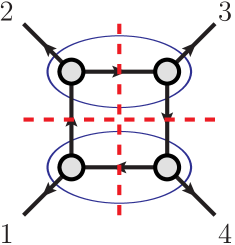
Refer to caption

Figure 5: The four-point quadruple cut. Two pairs of three-point amplitudes are grouped together (indicated by blue ovals) to form two easier-to-use four-point tree amplitudes. The cut propagators of the four-point tree amplitudes are canceled by multiplying by inverse propagators prior to imposing the cut conditions.

Moving on to the computation, we begin with the quadruple cut (Fig. 4a). The usual procedure is to sew four three-point amplitudes together, but working with three-point amplitudes in six dimensions can be complicated. It is, in fact, easier to multiply simpler four-point tree amplitudes by inverse propagators making them equivalent to the sum of products of two three-point amplitudes (Fig. 5), given the cut conditions. The quadruple cut is then

C1234subscript𝐶1234\displaystyle C_{1234} =statesA3(l1s,1,l2s)A3(l2s,2+,l3s)A3(l3s,3+,l4s)A3(l4s,4+,l1s)absentsubscriptstatessubscript𝐴3superscriptsubscript𝑙1𝑠superscript1superscriptsubscript𝑙2𝑠subscript𝐴3superscriptsubscript𝑙2𝑠superscript2superscriptsubscript𝑙3𝑠subscript𝐴3superscriptsubscript𝑙3𝑠superscript3superscriptsubscript𝑙4𝑠subscript𝐴3superscriptsubscript𝑙4𝑠superscript4superscriptsubscript𝑙1𝑠\displaystyle=\sum_{\mathrm{states}}A_{3}(-l_{1}^{s},1^{-},l_{2}^{s})A_{3}(-l_{2}^{s},2^{+},l_{3}^{s})A_{3}(-l_{3}^{s},3^{+},l_{4}^{s})A_{3}(-l_{4}^{s},4^{+},l_{1}^{s})
=states(i)2(l2p2)2(l2+p1)2A4(l2s,2+,3+,l4s)A4(l4s,4+,1,l2s).absentsubscriptstatessuperscript𝑖2superscriptsubscript𝑙2subscript𝑝22superscriptsubscript𝑙2subscript𝑝12subscript𝐴4superscriptsubscript𝑙2𝑠superscript2superscript3superscriptsubscript𝑙4𝑠subscript𝐴4superscriptsubscript𝑙4𝑠superscript4superscript1superscriptsubscript𝑙2𝑠\displaystyle=\sum_{\mathrm{states}}(-i)^{2}(l_{2}-p_{2})^{2}(l_{2}+p_{1})^{2}A_{4}(-l_{2}^{s},2^{+},3^{+},l_{4}^{s})A_{4}(-l_{4}^{s},4^{+},1^{-},l_{2}^{s}). (94)

The two-real-scalar two-gluon tree amplitude was given in eq. (28),

A4(0)(1aa˙g,2bb˙g,3s,4s)=14is12s231a2b3e3e[1a˙2b˙3e˙3e˙],superscriptsubscript𝐴40superscriptsubscript1𝑎˙𝑎𝑔superscriptsubscript2𝑏˙𝑏𝑔superscript3𝑠superscript4𝑠14𝑖subscript𝑠12subscript𝑠23delimited-⟨⟩subscript1𝑎subscript2𝑏subscript3𝑒superscript3𝑒delimited-[]subscript1˙𝑎subscript2˙𝑏subscript3˙𝑒superscript3˙𝑒A_{4}^{(0)}(1_{a\dot{a}}^{g},2_{b\dot{b}}^{g},3^{s},4^{s})=-\frac{1}{4}\frac{i}{s_{12}s_{23}}\langle 1_{a}2_{b}3_{e}3^{e}\rangle[1_{\dot{a}}2_{\dot{b}}3_{\dot{e}}3^{\dot{e}}], (95)

so the quadruple cut becomes

C1234=(l2)a,21,31,(l2)a[(l2)a˙,21˙,31˙,(l2)a˙](l4)b,41,12,(l4)b[(l4)b˙,41˙,12˙,(l4)b˙]16s232.subscript𝐶1234subscriptsubscript𝑙2𝑎subscript21subscript31superscriptsubscript𝑙2𝑎subscriptsubscript𝑙2˙𝑎subscript2˙1subscript3˙1superscriptsubscript𝑙2˙𝑎subscriptsubscript𝑙4𝑏subscript41subscript12superscriptsubscript𝑙4𝑏subscriptsubscript𝑙4˙𝑏subscript4˙1subscript1˙2superscriptsubscript𝑙4˙𝑏16superscriptsubscript𝑠232C_{1234}=\frac{\langle(-l_{2})_{a},2_{1},3_{1},(-l_{2})^{a}\rangle[(-l_{2})_{\dot{a}},2_{\dot{1}},3_{\dot{1}},(-l_{2})^{\dot{a}}]\langle(-l_{4})_{b},4_{1},1_{2},(-l_{4})^{b}\rangle[(-l_{4})_{\dot{b}},4_{\dot{1}},1_{\dot{2}},(-l_{4})^{\dot{b}}]}{16s_{23}^{2}}. (96)

The relevant spinor products are

(l2)1,21,31,(l2)1subscriptsubscript𝑙21subscript21subscript31superscriptsubscript𝑙21\displaystyle\langle(-l_{2})_{1},2_{1},3_{1},(-l_{2})^{1}\rangle =(l2)2,21,31,(l2)2=κ141 4[2 3],absentsubscriptsubscript𝑙22subscript21subscript31superscriptsubscript𝑙22subscript𝜅14delimited-⟨⟩14delimited-[]23\displaystyle=\langle(-l_{2})_{2},2_{1},3_{1},(-l_{2})^{2}\rangle=-\kappa_{14}\langle 1\,4\rangle[2\,3],
(l4)1,41,12,(l4)1subscriptsubscript𝑙41subscript41subscript12superscriptsubscript𝑙41\displaystyle\langle(-l_{4})_{1},4_{1},1_{2},(-l_{4})^{1}\rangle =(l4)2,41,12,(l4)2=t1 4[4 1],absentsubscriptsubscript𝑙42subscript41subscript12superscriptsubscript𝑙42𝑡delimited-⟨⟩14delimited-[]41\displaystyle=\langle(-l_{4})_{2},4_{1},1_{2},(-l_{4})^{2}\rangle=-t\langle 1\,4\rangle[4\,1],
[(l2)1˙,21˙,31˙,(l2)1˙]subscriptsubscript𝑙2˙1subscript2˙1subscript3˙1superscriptsubscript𝑙2˙1\displaystyle\mathrm{[}(-l_{2})_{\dot{1}},2_{\dot{1}},3_{\dot{1}},(-l_{2})^{\dot{1}}\mathrm{]} =[(l2)2˙,21˙,31˙,(l2)2˙]=κ141 4[2 3],absentsubscriptsubscript𝑙2˙2subscript2˙1subscript3˙1superscriptsubscript𝑙2˙2superscriptsubscript𝜅14delimited-⟨⟩14delimited-[]23\displaystyle=\mathrm{[}(-l_{2})_{\dot{2}},2_{\dot{1}},3_{\dot{1}},(-l_{2})^{\dot{2}}\mathrm{]}=\kappa_{14}^{\prime}\langle 1\,4\rangle[2\,3],
[(l4)1˙,41˙,12˙,(l4)1˙]subscriptsubscript𝑙4˙1subscript4˙1subscript1˙2superscriptsubscript𝑙4˙1\displaystyle\mathrm{[}(-l_{4})_{\dot{1}},4_{\dot{1}},1_{\dot{2}},(-l_{4})^{\dot{1}}\mathrm{]} =[(l4)2˙,41˙,12˙,(l4)2˙]=t1 4[4 1].absentsubscriptsubscript𝑙4˙2subscript4˙1subscript1˙2superscriptsubscript𝑙4˙2𝑡delimited-⟨⟩14delimited-[]41\displaystyle=\mathrm{[}(-l_{4})_{\dot{2}},4_{\dot{1}},1_{\dot{2}},(-l_{4})^{\dot{2}}\mathrm{]}=-t\langle 1\,4\rangle[4\,1]. (97)

Notice that we have not explicitly plugged in t=c1±𝑡superscriptsubscript𝑐1plus-or-minust=c_{1}^{\pm}. We recommend that this be done only at the end of the calculation as the square-roots tend to fall out when we average over solutions. Multiplying the products out, we arrive at

C1234=1s232κ14κ141 44[4 1]2[2 3]2t2.subscript𝐶12341superscriptsubscript𝑠232subscript𝜅14superscriptsubscript𝜅14superscriptdelimited-⟨⟩144superscriptdelimited-[]412superscriptdelimited-[]232superscript𝑡2C_{1234}=-\frac{1}{s_{23}^{2}}\kappa_{14}\kappa_{14}^{\prime}\langle 1\,4\rangle^{4}[4\,1]^{2}[2\,3]^{2}t^{2}. (98)

Now we take our sign convention into account using eq. (38) and average over solutions that take l3subscript𝑙3l_{3} on shell, i.e. t=c1±𝑡superscriptsubscript𝑐1plus-or-minust=c_{1}^{\pm}, arriving at

C4subscript𝐶4\displaystyle C_{4} =i2σC1234absent𝑖2subscript𝜎subscript𝐶1234\displaystyle=\frac{i}{2}\sum_{\sigma}C_{1234}
=imm~[2 4]2[1 2]2 33 4[4 1]s12s23s13(s12s232s13+mm~).absent𝑖𝑚~𝑚superscriptdelimited-[]242delimited-[]12delimited-⟨⟩23delimited-⟨⟩34delimited-[]41subscript𝑠12subscript𝑠23subscript𝑠13subscript𝑠12subscript𝑠232subscript𝑠13𝑚~𝑚\displaystyle=i\frac{m\tilde{m}[2\,4]^{2}}{[1\,2]\langle 2\,3\rangle\langle 3\,4\rangle[4\,1]}\frac{s_{12}s_{23}}{s_{13}}\left(\frac{s_{12}s_{23}}{2s_{13}}+m\tilde{m}\right). (99)

Associating mm~μ2𝑚~𝑚superscript𝜇2m\tilde{m}\rightarrow\mu^{2}, we see that the cut is nicely in the form of a polynomial in μ2superscript𝜇2\mu^{2}. We identify the coefficients,

C4[0]superscriptsubscript𝐶4delimited-[]0\displaystyle C_{4}^{[0]} =0,absent0\displaystyle=0,
C4[4]superscriptsubscript𝐶4delimited-[]4\displaystyle C_{4}^{[4]} =i[2 4]2[1 2]2 33 4[4 1]s12s23s13.absent𝑖superscriptdelimited-[]242delimited-[]12delimited-⟨⟩23delimited-⟨⟩34delimited-[]41subscript𝑠12subscript𝑠23subscript𝑠13\displaystyle=i\frac{[2\,4]^{2}}{[1\,2]\langle 2\,3\rangle\langle 3\,4\rangle[4\,1]}\frac{s_{12}s_{23}}{s_{13}}. (100)

These are in agreement with the previously known result BernMorgan .

Next we examine the triple cut in Fig. 4b to obtain triangle coefficients. Conveniently we have most of the cut for one of our momentum solutions from the box computation. We can use our quadruple cut in terms of the free parameter t𝑡t and multiply by the l3subscript𝑙3l_{3} propagator. This is the same as multiplying the three tree amplitudes in Fig. 4b together,

C124subscript𝐶124\displaystyle C_{124} =A3(l1s,1,l2s)A3(l2s,2+,3+,l4s)A3(l4s,4+,l1s)absentsubscript𝐴3superscriptsubscript𝑙1𝑠superscript1superscriptsubscript𝑙2𝑠subscript𝐴3superscriptsubscript𝑙2𝑠superscript2superscript3superscriptsubscript𝑙4𝑠subscript𝐴3superscriptsubscript𝑙4𝑠superscript4superscriptsubscript𝑙1𝑠\displaystyle=A_{3}(-l_{1}^{s},1^{-},l_{2}^{s})A_{3}(-l_{2}^{s},2^{+},3^{+},l_{4}^{s})A_{3}(-l_{4}^{s},4^{+},l_{1}^{s})
=C1234il32absentsubscript𝐶1234𝑖superscriptsubscript𝑙32\displaystyle=C_{1234}\frac{i}{l_{3}^{2}}
=i1s232κ14κ141 44[4 1]2[2 3]2t2(t4 2[1 2]+s12mm~ts141 2[4 2])1.absent𝑖1superscriptsubscript𝑠232subscript𝜅14superscriptsubscript𝜅14superscriptdelimited-⟨⟩144superscriptdelimited-[]412superscriptdelimited-[]232superscript𝑡2superscript𝑡delimited-⟨⟩42delimited-[]12subscript𝑠12𝑚~𝑚𝑡subscript𝑠14delimited-⟨⟩12delimited-[]421\displaystyle=-i\frac{1}{s_{23}^{2}}\kappa_{14}\kappa_{14}^{\prime}\langle 1\,4\rangle^{4}[4\,1]^{2}[2\,3]^{2}t^{2}\left(t\langle 4\,2\rangle[1\,2]+s_{12}-\frac{m\tilde{m}}{ts_{14}}\langle 1\,2\rangle[4\,2]\right)^{-1}. (101)

We also need the cut for the conjugate-momentum solution,

l¯1μ=12(t1|γμ|41tmm~s144|γμ|1).superscriptsubscript¯𝑙1absent𝜇12𝑡quantum-operator-productsuperscript1superscript𝛾𝜇superscript41𝑡𝑚~𝑚subscript𝑠14quantum-operator-productsuperscript4superscript𝛾𝜇superscript1\bar{l}_{1}^{*\mu}=\frac{1}{2}\left(t\langle 1^{-}|\gamma^{\mu}|4^{-}\rangle-\frac{1}{t}\frac{m\tilde{m}}{s_{14}}\langle 4^{-}|\gamma^{\mu}|1^{-}\rangle\right). (102)

Instead of defining new spinors and spinor products, we recognize that the conjugate solution is obtained from the original solution through the substitution tmm~ts14𝑡𝑚~𝑚𝑡subscript𝑠14t\rightarrow-\frac{m\tilde{m}}{ts_{14}}. We can then make this same substitution in the cut,

C124superscriptsubscript𝐶124\displaystyle C_{124}^{*} =C124|tmm~/ts14absentevaluated-atsubscript𝐶124𝑡𝑚~𝑚𝑡subscript𝑠14\displaystyle=C_{124}|_{t\rightarrow-m\tilde{m}/ts_{14}}
=i1s232κ14κ141 44[4 1]2[2 3]2(mm~)2t2s142(t1 2[4 2]+s12mm~ts144 2[1 2])1.absent𝑖1superscriptsubscript𝑠232subscript𝜅14superscriptsubscript𝜅14superscriptdelimited-⟨⟩144superscriptdelimited-[]412superscriptdelimited-[]232superscript𝑚~𝑚2superscript𝑡2superscriptsubscript𝑠142superscript𝑡delimited-⟨⟩12delimited-[]42subscript𝑠12𝑚~𝑚𝑡subscript𝑠14delimited-⟨⟩42delimited-[]121\displaystyle=-i\frac{1}{s_{23}^{2}}\kappa_{14}\kappa_{14}^{\prime}\langle 1\,4\rangle^{4}[4\,1]^{2}[2\,3]^{2}\frac{(m\tilde{m})^{2}}{t^{2}s_{14}^{2}}\left(t\langle 1\,2\rangle[4\,2]+s_{12}-\frac{m\tilde{m}}{ts_{14}}\langle 4\,2\rangle[1\,2]\right)^{-1}. (103)

Finally we perform an expansion around t𝑡t\rightarrow\infty as lined out in section IV.2, keeping only the order t0superscript𝑡0t^{0} term,

C3subscript𝐶3\displaystyle C_{3} =12{[Inft(C124)]|t0+[Inft(C124)]|t0}absent12evaluated-atdelimited-[]subscriptInf𝑡subscript𝐶124𝑡0evaluated-atdelimited-[]subscriptInf𝑡superscriptsubscript𝐶124𝑡0\displaystyle=-\frac{1}{2}\left\{[\mathrm{Inf}_{t}(C_{124})]|_{t\rightarrow 0}+[\mathrm{Inf}_{t}(C_{124}^{*})]|_{t\rightarrow 0}\right\}
=12{imm~[2 4]2[1 2]2 33 4[4 1]s12s232s132+0},absent12𝑖𝑚~𝑚superscriptdelimited-[]242delimited-[]12delimited-⟨⟩23delimited-⟨⟩34delimited-[]41subscript𝑠12superscriptsubscript𝑠232superscriptsubscript𝑠1320\displaystyle=-\frac{1}{2}\left\{-i\frac{m\tilde{m}[2\,4]^{2}}{[1\,2]\langle 2\,3\rangle\langle 3\,4\rangle[4\,1]}\frac{s_{12}s_{23}^{2}}{s_{13}^{2}}+0\right\}, (104)

which gives us the triangle coefficients,

C3;23[0]superscriptsubscript𝐶323delimited-[]0\displaystyle C_{3;23}^{[0]} =0,absent0\displaystyle=0,
C3;23[2]superscriptsubscript𝐶323delimited-[]2\displaystyle C_{3;23}^{[2]} =i2[2 4]2[1 2]2 33 4[4 1]s12s232s132,absent𝑖2superscriptdelimited-[]242delimited-[]12delimited-⟨⟩23delimited-⟨⟩34delimited-[]41subscript𝑠12superscriptsubscript𝑠232superscriptsubscript𝑠132\displaystyle=\frac{i}{2}\frac{[2\,4]^{2}}{[1\,2]\langle 2\,3\rangle\langle 3\,4\rangle[4\,1]}\frac{s_{12}s_{23}^{2}}{s_{13}^{2}}, (105)

where “23” indicates that legs 2 and 3 have been “pinched” to form the triangle.

We also need the triangle contributions from other triple-cut configurations. To pinch legs 3 and 4, we use the momentum solution,

l¯2μ=12(t1|γμ|21tmm~s122|γμ|1),superscriptsubscript¯𝑙2𝜇12𝑡quantum-operator-productsuperscript1superscript𝛾𝜇superscript21𝑡𝑚~𝑚subscript𝑠12quantum-operator-productsuperscript2superscript𝛾𝜇superscript1\displaystyle\bar{l}_{2}^{\mu}=\frac{1}{2}\left(t\langle 1^{-}|\gamma^{\mu}|2^{-}\rangle-\frac{1}{t}\frac{m\tilde{m}}{s_{12}}\langle 2^{-}|\gamma^{\mu}|1^{-}\rangle\right), (106)

along with its conjugate solution. We define spinors and spinor products (many of which can be found through simple relabellings of our previous results) using this momentum solution and calculate cuts in a similar manner. The remaining triangle coefficients are then

C3;12[0]=C3;34[0]=C3;41[0]=0,superscriptsubscript𝐶312delimited-[]0superscriptsubscript𝐶334delimited-[]0superscriptsubscript𝐶341delimited-[]00\displaystyle C_{3;12}^{[0]}=C_{3;34}^{[0]}=C_{3;41}^{[0]}=0,
C3;12[2]superscriptsubscript𝐶312delimited-[]2\displaystyle C_{3;12}^{[2]} =i2[2 4]2[1 2]2 33 4[4 1](s233s132+2s232s13s23),absent𝑖2superscriptdelimited-[]242delimited-[]12delimited-⟨⟩23delimited-⟨⟩34delimited-[]41superscriptsubscript𝑠233superscriptsubscript𝑠1322superscriptsubscript𝑠232subscript𝑠13subscript𝑠23\displaystyle=\frac{i}{2}\frac{[2\,4]^{2}}{[1\,2]\langle 2\,3\rangle\langle 3\,4\rangle[4\,1]}\left(\frac{s_{23}^{3}}{s_{13}^{2}}+2\frac{s_{23}^{2}}{s_{13}}-s_{23}\right),
C3;34[2]superscriptsubscript𝐶334delimited-[]2\displaystyle C_{3;34}^{[2]} =i2[2 4]2[1 2]2 33 4[4 1]s122s23s132,absent𝑖2superscriptdelimited-[]242delimited-[]12delimited-⟨⟩23delimited-⟨⟩34delimited-[]41superscriptsubscript𝑠122subscript𝑠23superscriptsubscript𝑠132\displaystyle=\frac{i}{2}\frac{[2\,4]^{2}}{[1\,2]\langle 2\,3\rangle\langle 3\,4\rangle[4\,1]}\frac{s_{12}^{2}s_{23}}{s_{13}^{2}},
C3;41[2]superscriptsubscript𝐶341delimited-[]2\displaystyle C_{3;41}^{[2]} =i2[2 4]2[1 2]2 33 4[4 1](s123s132+2s122s13s12).absent𝑖2superscriptdelimited-[]242delimited-[]12delimited-⟨⟩23delimited-⟨⟩34delimited-[]41superscriptsubscript𝑠123superscriptsubscript𝑠1322superscriptsubscript𝑠122subscript𝑠13subscript𝑠12\displaystyle=\frac{i}{2}\frac{[2\,4]^{2}}{[1\,2]\langle 2\,3\rangle\langle 3\,4\rangle[4\,1]}\left(\frac{s_{12}^{3}}{s_{13}^{2}}+2\frac{s_{12}^{2}}{s_{13}}-s_{12}\right). (107)

Triangle integrals are dependent only on their kinematic invariant masses, so certain pairs of integrals corresponding to the above coefficients are in fact equal. For the one-mass triangle with invariant mass square s12=(p1+p2)2=s34subscript𝑠12superscriptsubscript𝑝1subscript𝑝22subscript𝑠34s_{12}=(p_{1}+p_{2})^{2}=s_{34},

I3;s1242ϵ[f(μ2)]=I3;1242ϵ[f(μ2)]=I3;3442ϵ[f(μ2)].superscriptsubscript𝐼3subscript𝑠1242italic-ϵdelimited-[]𝑓superscript𝜇2superscriptsubscript𝐼31242italic-ϵdelimited-[]𝑓superscript𝜇2superscriptsubscript𝐼33442italic-ϵdelimited-[]𝑓superscript𝜇2\displaystyle I_{3;s_{12}}^{4-2\epsilon}[f(\mu^{2})]=I_{3;12}^{4-2\epsilon}[f(\mu^{2})]=I_{3;34}^{4-2\epsilon}[f(\mu^{2})]. (108)

It then makes sense to write only one coefficient C3;s12=C3;12+C3;34subscript𝐶3subscript𝑠12subscript𝐶312subscript𝐶334C_{3;s_{12}}=C_{3;12}+C_{3;34}. In this basis our results are

C3;s12[2]=i[2 4]2[1 2]2 33 4[4 1]s232s132(s13s12),superscriptsubscript𝐶3subscript𝑠12delimited-[]2𝑖superscriptdelimited-[]242delimited-[]12delimited-⟨⟩23delimited-⟨⟩34delimited-[]41superscriptsubscript𝑠232superscriptsubscript𝑠132subscript𝑠13subscript𝑠12\displaystyle C_{3;s_{12}}^{[2]}=i\frac{[2\,4]^{2}}{[1\,2]\langle 2\,3\rangle\langle 3\,4\rangle[4\,1]}\frac{s_{23}^{2}}{s_{13}^{2}}(s_{13}-s_{12}),
C3;s23[2]=i[2 4]2[1 2]2 33 4[4 1]s122s132(s13s23).superscriptsubscript𝐶3subscript𝑠23delimited-[]2𝑖superscriptdelimited-[]242delimited-[]12delimited-⟨⟩23delimited-⟨⟩34delimited-[]41superscriptsubscript𝑠122superscriptsubscript𝑠132subscript𝑠13subscript𝑠23\displaystyle C_{3;s_{23}}^{[2]}=i\frac{[2\,4]^{2}}{[1\,2]\langle 2\,3\rangle\langle 3\,4\rangle[4\,1]}\frac{s_{12}^{2}}{s_{13}^{2}}(s_{13}-s_{23}). (109)

Finally we calculate the bubble integral coefficients using double and triple cuts. For this special case, dependence on y𝑦y in the spinor products falls out and the products for these cuts are also given by eq. (97) (this is of course not generally true). We can then take the quadruple cut (98) and multiply by propagators for l1subscript𝑙1l_{1} and l3subscript𝑙3l_{3} to obtain the two-particle cut,

C24=subscript𝐶24absent\displaystyle C_{24}= A4(l2s,2+,3+,l4s)A4(l4s,4+,1,l2s)subscript𝐴4superscriptsubscript𝑙2𝑠superscript2superscript3superscriptsubscript𝑙4𝑠subscript𝐴4superscriptsubscript𝑙4𝑠superscript4superscript1superscriptsubscript𝑙2𝑠\displaystyle A_{4}(-l_{2}^{s},2^{+},3^{+},l_{4}^{s})A_{4}(-l_{4}^{s},4^{+},1^{-},l_{2}^{s})
=\displaystyle= C1234il12il32subscript𝐶1234𝑖superscriptsubscript𝑙12𝑖superscriptsubscript𝑙32\displaystyle C_{1234}\frac{i}{l_{1}^{2}}\frac{i}{l_{3}^{2}}
=\displaystyle= 1s232κ14κ141 44[4 1]2[2 3]2t2((1y)s14)11superscriptsubscript𝑠232subscript𝜅14superscriptsubscript𝜅14superscriptdelimited-⟨⟩144superscriptdelimited-[]412superscriptdelimited-[]232superscript𝑡2superscript1𝑦subscript𝑠141\displaystyle\frac{1}{s_{23}^{2}}\kappa_{14}\kappa_{14}^{\prime}\langle 1\,4\rangle^{4}[4\,1]^{2}[2\,3]^{2}t^{2}(-(1-y)s_{14})^{-1}
×(ys12+(1y)s13+t4 3[3 1]+(y(1y)tmm~ts14)1 3[3 4])1.absentsuperscript𝑦subscript𝑠121𝑦subscript𝑠13𝑡delimited-⟨⟩43delimited-[]31𝑦1𝑦𝑡𝑚~𝑚𝑡subscript𝑠14delimited-⟨⟩13delimited-[]341\displaystyle\times\left(ys_{12}+(1-y)s_{13}+t\langle 4\,3\rangle[3\,1]+\left(\frac{y(1-y)}{t}-\frac{m\tilde{m}}{ts_{14}}\right)\langle 1\,3\rangle[3\,4]\right)^{-1}. (110)

According to eq. (48), the two-particle cut contribution to the bubble coefficient is

i[Inft[InfyA1A2](y)](t)|t0,ymYm.evaluated-at𝑖delimited-[]subscriptInf𝑡delimited-[]subscriptInf𝑦subscript𝐴1subscript𝐴2𝑦𝑡formulae-sequence𝑡0superscript𝑦𝑚subscript𝑌𝑚\displaystyle-i[\mathrm{Inf}_{t}[\mathrm{Inf}_{y}A_{1}A_{2}](y)](t)|_{t\rightarrow 0,y^{m}\rightarrow Y_{m}}. (111)

Expanding C24subscript𝐶24C_{24} around infinity in y𝑦y, we find

InfyC24=0,subscriptInf𝑦subscript𝐶240\displaystyle\mathrm{Inf}_{y}C_{24}=0, (112)

so the contribution in this case is 00.

Refer to caption
(a)
Refer to caption
(b)
Figure 6: Triple cuts contributing to the four-point amplitude bubble coefficient for the s23subscript𝑠23s_{23}-channel bubble integral.

We also need to examine three-particle cuts that share two on-shell conditions with our double cut, as explained in section IV.3. The two possible configurations are shown in Fig. 6. Fig. 6a makes no contribution due to our convenient choice of momentum parametrization. Any contribution must be proportional to T1subscript𝑇1T_{1}, T2subscript𝑇2T_{2} and T3subscript𝑇3T_{3} as given in eq. (50). Recall that for our momentum solution, K1=p4superscriptsubscript𝐾1subscript𝑝4K_{1}^{\flat}=p_{4}, and in Fig. 6a, K3=p4subscript𝐾3subscript𝑝4K_{3}=p_{4}. We then find that T1=T2=T3=0subscript𝑇1subscript𝑇2subscript𝑇30T_{1}=T_{2}=T_{3}=0, and the contribution from this particular triple cut vanishes.

The only bubble contribution then comes from Fig. 6b, where K3=p3subscript𝐾3subscript𝑝3K_{3}=p_{3}. To make use of eq. (48), we need to find the solutions to the parameter y𝑦y that take the third leg l3subscript𝑙3l_{3} on shell. These are given by eq. (46),

y±=B1±B12+4B0B22B2,subscript𝑦plus-or-minusplus-or-minussubscript𝐵1superscriptsubscript𝐵124subscript𝐵0subscript𝐵22subscript𝐵2\displaystyle y_{\pm}=\frac{B_{1}\pm\sqrt{B_{1}^{2}+4B_{0}B_{2}}}{2B_{2}}, (113)

where

B2subscript𝐵2\displaystyle B_{2} =s231 3[3 4],absentsubscript𝑠23delimited-⟨⟩13delimited-[]34\displaystyle=s_{23}\langle 1\,3\rangle[3\,4],
B1subscript𝐵1\displaystyle B_{1} =s23t(s12s13)+s231 3[3 4],absentsubscript𝑠23𝑡subscript𝑠12subscript𝑠13subscript𝑠23delimited-⟨⟩13delimited-[]34\displaystyle=s_{23}t(s_{12}-s_{13})+s_{23}\langle 1\,3\rangle[3\,4],
B0subscript𝐵0\displaystyle B_{0} =s23t24 3[3 1]μ21 3[3 4]+s13s23t.absentsubscript𝑠23superscript𝑡2delimited-⟨⟩43delimited-[]31superscript𝜇2delimited-⟨⟩13delimited-[]34subscript𝑠13subscript𝑠23𝑡\displaystyle=s_{23}t^{2}\langle 4\,3\rangle[3\,1]-\mu^{2}\langle 1\,3\rangle[3\,4]+s_{13}s_{23}t. (114)

Our cut is given by

C234subscript𝐶234\displaystyle C_{234} =A4(l4s,4+,1,l2s)A3(l2s,2+,l3s)A3(l3s,3+,l4s)absentsubscript𝐴4superscriptsubscript𝑙4𝑠superscript4superscript1superscriptsubscript𝑙2𝑠subscript𝐴3superscriptsubscript𝑙2𝑠superscript2superscriptsubscript𝑙3𝑠subscript𝐴3superscriptsubscript𝑙3𝑠superscript3superscriptsubscript𝑙4𝑠\displaystyle=A_{4}(-l_{4}^{s},4^{+},1^{-},l_{2}^{s})A_{3}(-l_{2}^{s},2^{+},l_{3}^{s})A_{3}(-l_{3}^{s},3^{+},l_{4}^{s})
=C1234il12absentsubscript𝐶1234𝑖superscriptsubscript𝑙12\displaystyle=C_{1234}\frac{i}{l_{1}^{2}}
=i1s142κ14κ141 44[4 1]2[2 3]2t2((1y)s14)1.absent𝑖1superscriptsubscript𝑠142subscript𝜅14superscriptsubscript𝜅14superscriptdelimited-⟨⟩144superscriptdelimited-[]412superscriptdelimited-[]232superscript𝑡2superscript1𝑦subscript𝑠141\displaystyle=-i\frac{1}{s_{14}^{2}}\kappa_{14}\kappa_{14}^{\prime}\langle 1\,4\rangle^{4}[4\,1]^{2}[2\,3]^{2}t^{2}(-(1-y)s_{14})^{-1}. (115)

Plugging in the solutions for y𝑦y and expanding in t𝑡t, we find

12σy[InftC234](t)=i2mm~1 3[2 3][3 4]2 3s13s12s12s13t+O(t0).12subscriptsubscript𝜎𝑦delimited-[]subscriptInf𝑡subscript𝐶234𝑡𝑖2𝑚~𝑚delimited-⟨⟩13delimited-[]23delimited-[]34delimited-⟨⟩23subscript𝑠13subscript𝑠12subscript𝑠12subscript𝑠13𝑡𝑂superscript𝑡0\displaystyle\frac{1}{2}\sum_{\sigma_{y}}[\mathrm{Inf}_{t}C_{234}](t)=\frac{i}{2}\frac{m\tilde{m}\langle 1\,3\rangle[2\,3][3\,4]}{\langle 2\,3\rangle}\frac{s_{13}-s_{12}}{s_{12}s_{13}}t+O(t^{0}). (116)

Lastly we need to take tT1𝑡subscript𝑇1t\rightarrow T_{1}, where T1subscript𝑇1T_{1} is given by eq. (50),

T1=21 3[3 4]s232.subscript𝑇12delimited-⟨⟩13delimited-[]34superscriptsubscript𝑠232\displaystyle T_{1}=-2\frac{\langle 1\,3\rangle[3\,4]}{s_{23}^{2}}. (117)

We then have the full coefficient expression,

C2subscript𝐶2\displaystyle C_{2} =i[Inft[InfyA1A2](y)](t)|t0,ymYm12Ctriσy[InftA1A2A3](t)|tjTjabsentevaluated-at𝑖delimited-[]subscriptInf𝑡delimited-[]subscriptInf𝑦subscript𝐴1subscript𝐴2𝑦𝑡formulae-sequence𝑡0superscript𝑦𝑚subscript𝑌𝑚evaluated-at12subscriptsubscript𝐶trisubscriptsubscript𝜎𝑦delimited-[]subscriptInf𝑡subscript𝐴1subscript𝐴2subscript𝐴3𝑡superscript𝑡𝑗subscript𝑇𝑗\displaystyle=-i[\mathrm{Inf}_{t}[\mathrm{Inf}_{y}A_{1}A_{2}](y)](t)|_{t\rightarrow 0,y^{m}\rightarrow Y_{m}}-\frac{1}{2}\sum_{C_{\mathrm{tri}}}\sum_{\sigma_{y}}[\mathrm{Inf}_{t}A_{1}A_{2}A_{3}](t)|_{t^{j}\rightarrow T_{j}}
=imm~[2 4]2[1 2]2 33 4[4 1]s12s13s23(s13s12),absent𝑖𝑚~𝑚superscriptdelimited-[]242delimited-[]12delimited-⟨⟩23delimited-⟨⟩34delimited-[]41subscript𝑠12subscript𝑠13subscript𝑠23subscript𝑠13subscript𝑠12\displaystyle=i\frac{m\tilde{m}[2\,4]^{2}}{[1\,2]\langle 2\,3\rangle\langle 3\,4\rangle[4\,1]}\frac{s_{12}}{s_{13}s_{23}}(s_{13}-s_{12}), (118)

resulting in the coefficients,

C2;23[0]superscriptsubscript𝐶223delimited-[]0\displaystyle C_{2;23}^{[0]} =0,absent0\displaystyle=0,
C2;23[2]superscriptsubscript𝐶223delimited-[]2\displaystyle C_{2;23}^{[2]} =i[2 4]2[1 2]2 33 4[4 1]s12s13s23(s13s12).absent𝑖superscriptdelimited-[]242delimited-[]12delimited-⟨⟩23delimited-⟨⟩34delimited-[]41subscript𝑠12subscript𝑠13subscript𝑠23subscript𝑠13subscript𝑠12\displaystyle=i\frac{[2\,4]^{2}}{[1\,2]\langle 2\,3\rangle\langle 3\,4\rangle[4\,1]}\frac{s_{12}}{s_{13}s_{23}}(s_{13}-s_{12}). (119)

Through a similar computation, we find the coefficients for an invariant mass in the s12subscript𝑠12s_{12} channel,

C2;12[0]superscriptsubscript𝐶212delimited-[]0\displaystyle C_{2;12}^{[0]} =0,absent0\displaystyle=0,
C2;12[2]superscriptsubscript𝐶212delimited-[]2\displaystyle C_{2;12}^{[2]} =i[2 4]2[1 2]2 33 4[4 1]s23s12s13(s13s23).absent𝑖superscriptdelimited-[]242delimited-[]12delimited-⟨⟩23delimited-⟨⟩34delimited-[]41subscript𝑠23subscript𝑠12subscript𝑠13subscript𝑠13subscript𝑠23\displaystyle=i\frac{[2\,4]^{2}}{[1\,2]\langle 2\,3\rangle\langle 3\,4\rangle[4\,1]}\frac{s_{23}}{s_{12}s_{13}}(s_{13}-s_{23}). (120)

All coefficients are in agreement with the previously known result BernMorgan .

V.4 Gluon loop

Next we look at A4(1)(1,2+,3+,4+)superscriptsubscript𝐴41superscript1superscript2superscript3superscript4A_{4}^{(1)}(1^{-},2^{+},3^{+},4^{+}) with a gluon loop. Unlike the scalar-loop amplitude, the gluon-loop amplitude requires a state-sum reduction to reduce from six dimensions to the FDH scheme. Gluons in six dimensions have two additional polarization states compared to four dimensions. The extra contribution of these states manifests itself in a term proportional to the dimension of spacetime, which is then the term that we must reduce. We will find that we must subtract twice the contribution of the scalar-loop diagram to reduce from six dimensions to the FDH scheme. The reasoning behind this can be found in ref. FullOneLoopGiele . We summarize the argument before presenting the results of A4(1)(1,2+,3+,4+)superscriptsubscript𝐴41superscript1superscript2superscript3superscript4A_{4}^{(1)}(1^{-},2^{+},3^{+},4^{+}).

The dependence of a one-loop coefficient on the dimensionality of spacetime is at most linear. Such terms arise from a closed loop of contracted metric tensors and/or gamma matrices from vertices and propagators making up the loop. We can therefore separate coefficients into pieces dependent on D𝐷D and pieces independent of it,

C(D)=CI+DCD.superscript𝐶𝐷subscript𝐶𝐼𝐷subscript𝐶𝐷\displaystyle C^{(D)}=C_{I}+DC_{D}. (121)

As the authors of ref. FullOneLoopGiele point out, this can be used to find the coefficients in the FDH scheme by finding the coefficients in two dimensions D>4𝐷4D>4: D1subscript𝐷1D_{1} and D2subscript𝐷2D_{2} (doing the full calculation in D=4𝐷4D=4 of course loses the non-cut-constructible terms), then solving for CIsubscript𝐶𝐼C_{I} and CDsubscript𝐶𝐷C_{D},

CIsubscript𝐶𝐼\displaystyle C_{I} =D2C(D1)D1C(D2)D2D1,absentsubscript𝐷2superscript𝐶subscript𝐷1subscript𝐷1superscript𝐶subscript𝐷2subscript𝐷2subscript𝐷1\displaystyle=\frac{D_{2}C^{(D_{1})}-D_{1}C^{(D_{2})}}{D_{2}-D_{1}},
CDsubscript𝐶𝐷\displaystyle C_{D} =C(D2)C(D1)D2D1.absentsuperscript𝐶subscript𝐷2superscript𝐶subscript𝐷1subscript𝐷2subscript𝐷1\displaystyle=\frac{C^{(D_{2})}-C^{(D_{1})}}{D_{2}-D_{1}}. (122)

The coefficient in the FDH scheme is then FullOneLoopGiele

CFDH=D2C(D2)D1C(D2)D2D1+4C(D2)C(D1)D2D1.superscript𝐶FDHsubscript𝐷2superscript𝐶subscript𝐷2subscript𝐷1superscript𝐶subscript𝐷2subscript𝐷2subscript𝐷14superscript𝐶subscript𝐷2superscript𝐶subscript𝐷1subscript𝐷2subscript𝐷1\displaystyle C^{\mathrm{FDH}}=\frac{D_{2}C^{(D_{2})}-D_{1}C^{(D_{2})}}{D_{2}-D_{1}}+4\frac{C^{(D_{2})}-C^{(D_{1})}}{D_{2}-D_{1}}. (123)

With this fact in mind, the authors of ref. FullOneLoopGiele study the gluon-loop amplitudes in five and six dimensions and show that they differ in a rather simple way. Suppose we calculate in D=5𝐷5D=5 with five-dimensional loop momentum. We will have three polarization states of the internal gluons, and we will obtain coefficients for five dimensions. Now suppose we upgrade to D=6𝐷6D=6 but leave our loop momentum in five dimensions. We view this as being the same loop momentum as in the D=5𝐷5D=5 case; the only difference is now we have added an additional polarization state of the gluon, which can be thought of as being along the sixth dimension of six-dimensional space.

It should be noted that the restriction on the loop momentum does not prevent us from obtaining the correct D=6𝐷6D=6 coefficient; problems arise only when we take it down to four dimensions. This can be understood through a fact mentioned in Appendix A: the loop momentum components beyond four dimensions only enter coefficients in a particular combination through contractions of the loop momentum with itself,

l~2=l2l¯2,superscript~𝑙2superscript𝑙2superscript¯𝑙2\tilde{l}^{2}=l^{2}-\bar{l}^{2}, (124)

where l¯¯𝑙\bar{l} and l~~𝑙\tilde{l} are the four- and (D4)𝐷4(D-4)-dimensional pieces of the loop momentum respectively. As long as we do not set this to 00, we find the full coefficient (for a more in depth discussion see ref. FullOneLoopGiele ).

So, the contribution to the D=6𝐷6D=6 coefficient due to the extra polarization state (with polarization along the sixth dimension) is exactly the difference between the D=5𝐷5D=5 and D=6𝐷6D=6 coefficients. To see what this difference is, we go to the Feynman rules.

A relevant three-gluon vertex, with polarizations taken into account, is

i2(ημν(kl2)ρ+ηνρ(l2l1)μ+ηρμ(l1k)ν)ϵkμϵl2νϵl1ρ,𝑖2superscript𝜂𝜇𝜈superscript𝑘subscript𝑙2𝜌superscript𝜂𝜈𝜌superscriptsubscript𝑙2subscript𝑙1𝜇superscript𝜂𝜌𝜇superscriptsubscript𝑙1𝑘𝜈subscriptitalic-ϵ𝑘𝜇subscriptitalic-ϵsubscript𝑙2𝜈subscriptitalic-ϵsubscript𝑙1𝜌\frac{i}{\sqrt{2}}(\eta^{\mu\nu}(k-l_{2})^{\rho}+\eta^{\nu\rho}(l_{2}-l_{1})^{\mu}+\eta^{\rho\mu}(l_{1}-k)^{\nu})\epsilon_{k\mu}\epsilon_{l_{2}\nu}\epsilon_{l_{1}\rho}, (125)

where k𝑘k is an outgoing external momentum and l1subscript𝑙1l_{1} and l2subscript𝑙2l_{2} are outgoing internal loop momenta. We wish to examine the contribution from the polarization in the sixth dimension, so we look at only those components of ϵl1subscriptitalic-ϵsubscript𝑙1\epsilon_{l_{1}} and ϵl2subscriptitalic-ϵsubscript𝑙2\epsilon_{l_{2}}. When these are contracted with ϵksubscriptitalic-ϵ𝑘\epsilon_{k}, k𝑘k, l1subscript𝑙1l_{1} or l2subscript𝑙2l_{2}, they vanish since none of those vectors contain a sixth-dimensional component. The only non-vanishing contraction is that between the sixth-dimensional components of ϵl1subscriptitalic-ϵsubscript𝑙1\epsilon_{l_{1}} and ϵl2subscriptitalic-ϵsubscript𝑙2\epsilon_{l_{2}}. Our vertex then becomes

i2ϵl1,6ϵl2,6ϵk(l2l1)=i2ϵk(l2l1),𝑖2subscriptitalic-ϵsubscript𝑙16subscriptitalic-ϵsubscript𝑙26subscriptitalic-ϵ𝑘subscript𝑙2subscript𝑙1𝑖2subscriptitalic-ϵ𝑘subscript𝑙2subscript𝑙1\frac{i}{\sqrt{2}}\,\epsilon_{l_{1},6}\cdot\epsilon_{l_{2},6}\,\,\epsilon_{k}\cdot(l_{2}-l_{1})=\frac{i}{\sqrt{2}}\epsilon_{k}\cdot(l_{2}-l_{1}), (126)

up to a sign depending on the normalization of the polarization vectors. This is the two-real-scalar gluon vertex with polarization of the gluon included. Therefore the contribution of the polarization in the sixth dimension is equal to that of a scalar particle, and the D=5𝐷5D=5 and D=6𝐷6D=6 coefficients differ by a coefficient found using cuts where the internal gluon loop has been replaced by a scalar loop,

C(6)=C(5)+Cscalar.superscript𝐶6superscript𝐶5superscript𝐶scalarC^{(6)}=C^{(5)}+C^{\mathrm{scalar}}. (127)

For our FDH coefficient then, we find

CFDH=C(6)2Cscalar.superscript𝐶FDHsuperscript𝐶62superscript𝐶scalar\displaystyle C^{\mathrm{FDH}}=C^{(6)}-2C^{\mathrm{scalar}}. (128)

Coefficients in the FDH scheme can be found from six-dimensional coefficients by subtracting twice the contribution of a scalar-loop diagram. (Here we only studied the three-gluon vertex. Similar arguments can be used for a four-gluon vertex; in fact, it is true that any n𝑛n-gluon tree amplitude with two gluons polarized along the sixth dimension is equivalent to a tree amplitude with n2𝑛2n-2 gluons and two scalars FullOneLoopGiele .) This leads us to the physical interpretation that the polarization states in six dimensions consist of the polarization states of four dimensions plus two scalars, but that they may be mixed in some nontrivial way. We will not necessarily be able to identify the state a=1𝑎1a=1, a˙=1˙˙𝑎˙1\dot{a}=\dot{1} in six dimensions, for example, with a state in four dimensions.

We now turn to the coefficients of A4(1)(1,2+,3+,4+)superscriptsubscript𝐴41superscript1superscript2superscript3superscript4A_{4}^{(1)}(1^{-},2^{+},3^{+},4^{+}) with a gluon loop and show that our state-sum reduction procedure works. Using the four-gluon tree amplitude (26), the quadruple cut is

C1234subscript𝐶1234\displaystyle C_{1234} =states(i)2(l2p2)2(l2+p1)2A4(l2g,2+,3+,l4g)A4(l4g,4+,1,l2g)absentsubscriptstatessuperscript𝑖2superscriptsubscript𝑙2subscript𝑝22superscriptsubscript𝑙2subscript𝑝12subscript𝐴4superscriptsubscript𝑙2𝑔superscript2superscript3superscriptsubscript𝑙4𝑔subscript𝐴4superscriptsubscript𝑙4𝑔superscript4superscript1superscriptsubscript𝑙2𝑔\displaystyle=\sum_{\mathrm{states}}(-i)^{2}(l_{2}-p_{2})^{2}(l_{2}+p_{1})^{2}A_{4}(-l_{2}^{g},2^{+},3^{+},l_{4}^{g})A_{4}(-l_{4}^{g},4^{+},1^{-},l_{2}^{g})
=(l2)a,21,31,(l4)b[(l2)a˙,21˙,31˙,(l4)b˙](l4)b,41,12,(l2)a[(l4)b˙,41˙,12˙,(l2)a˙]s232.absentsubscriptsubscript𝑙2𝑎subscript21subscript31subscriptsubscript𝑙4𝑏subscriptsubscript𝑙2˙𝑎subscript2˙1subscript3˙1subscriptsubscript𝑙4˙𝑏superscriptsubscript𝑙4𝑏subscript41subscript12superscriptsubscript𝑙2𝑎superscriptsubscript𝑙4˙𝑏subscript4˙1subscript1˙2superscriptsubscript𝑙2˙𝑎superscriptsubscript𝑠232\displaystyle=\frac{\langle(-l_{2})_{a},2_{1},3_{1},(l_{4})_{b}\rangle[(-l_{2})_{\dot{a}},2_{\dot{1}},3_{\dot{1}},(l_{4})_{\dot{b}}]\langle(-l_{4})^{b},4_{1},1_{2},(l_{2})^{a}\rangle[(-l_{4})^{\dot{b}},4_{\dot{1}},1_{\dot{2}},(l_{2})^{\dot{a}}]}{s_{23}^{2}}. (129)

The spinor products required for this calculation are in eqs. (86) and (92). In a manner similar to the scalar-loop calculation, we find all of the integral coefficients for the gluon-loop amplitude. All scalar integral coefficients vanish, and we have

C4[4],6Dsuperscriptsubscript𝐶4delimited-[]46𝐷\displaystyle C_{4}^{[4],6D} =4i[2 4]2[1 2]2 33 4[4 1]s12s23s13,absent4𝑖superscriptdelimited-[]242delimited-[]12delimited-⟨⟩23delimited-⟨⟩34delimited-[]41subscript𝑠12subscript𝑠23subscript𝑠13\displaystyle=4i\frac{[2\,4]^{2}}{[1\,2]\langle 2\,3\rangle\langle 3\,4\rangle[4\,1]}\frac{s_{12}s_{23}}{s_{13}},
C3;s12[2],6Dsuperscriptsubscript𝐶3subscript𝑠12delimited-[]26𝐷\displaystyle C_{3;s_{12}}^{[2],6D} =4i[2 4]2[1 2]2 33 4[4 1]s232s132(s13s12),absent4𝑖superscriptdelimited-[]242delimited-[]12delimited-⟨⟩23delimited-⟨⟩34delimited-[]41superscriptsubscript𝑠232superscriptsubscript𝑠132subscript𝑠13subscript𝑠12\displaystyle=4i\frac{[2\,4]^{2}}{[1\,2]\langle 2\,3\rangle\langle 3\,4\rangle[4\,1]}\frac{s_{23}^{2}}{s_{13}^{2}}(s_{13}-s_{12}),
C3;s23[2],6Dsuperscriptsubscript𝐶3subscript𝑠23delimited-[]26𝐷\displaystyle C_{3;s_{23}}^{[2],6D} =4i[2 4]2[1 2]2 33 4[4 1]s122s132(s13s23),absent4𝑖superscriptdelimited-[]242delimited-[]12delimited-⟨⟩23delimited-⟨⟩34delimited-[]41superscriptsubscript𝑠122superscriptsubscript𝑠132subscript𝑠13subscript𝑠23\displaystyle=4i\frac{[2\,4]^{2}}{[1\,2]\langle 2\,3\rangle\langle 3\,4\rangle[4\,1]}\frac{s_{12}^{2}}{s_{13}^{2}}(s_{13}-s_{23}),
C2;12[2],6Dsuperscriptsubscript𝐶212delimited-[]26𝐷\displaystyle C_{2;12}^{[2],6D} =4i[2 4]2[1 2]2 33 4[4 1]s23s12s13(s13s23),absent4𝑖superscriptdelimited-[]242delimited-[]12delimited-⟨⟩23delimited-⟨⟩34delimited-[]41subscript𝑠23subscript𝑠12subscript𝑠13subscript𝑠13subscript𝑠23\displaystyle=4i\frac{[2\,4]^{2}}{[1\,2]\langle 2\,3\rangle\langle 3\,4\rangle[4\,1]}\frac{s_{23}}{s_{12}s_{13}}(s_{13}-s_{23}),
C2;23[2],6Dsuperscriptsubscript𝐶223delimited-[]26𝐷\displaystyle C_{2;23}^{[2],6D} =4i[2 4]2[1 2]2 33 4[4 1]s12s13s23(s13s12).absent4𝑖superscriptdelimited-[]242delimited-[]12delimited-⟨⟩23delimited-⟨⟩34delimited-[]41subscript𝑠12subscript𝑠13subscript𝑠23subscript𝑠13subscript𝑠12\displaystyle=4i\frac{[2\,4]^{2}}{[1\,2]\langle 2\,3\rangle\langle 3\,4\rangle[4\,1]}\frac{s_{12}}{s_{13}s_{23}}(s_{13}-s_{12}). (130)

Rational terms for a gluon-loop amplitude are equal to twice the rational terms for a scalar-loop amplitude Badger , so it is not surprising that the six-dimensional coefficients for the gluon loop are 4 times those for the scalar loop (this is not true for cut-constructible pieces). Subtracting twice the scalar-loop coefficients in section V.3 from eq. (130) according to our prescription, we arrive at our coefficients in the FDH scheme,

C4[4]superscriptsubscript𝐶4delimited-[]4\displaystyle C_{4}^{[4]} =2i[2 4]2[1 2]2 33 4[4 1]s12s23s13,absent2𝑖superscriptdelimited-[]242delimited-[]12delimited-⟨⟩23delimited-⟨⟩34delimited-[]41subscript𝑠12subscript𝑠23subscript𝑠13\displaystyle=2i\frac{[2\,4]^{2}}{[1\,2]\langle 2\,3\rangle\langle 3\,4\rangle[4\,1]}\frac{s_{12}s_{23}}{s_{13}},
C3;s12[2]superscriptsubscript𝐶3subscript𝑠12delimited-[]2\displaystyle C_{3;s_{12}}^{[2]} =2i[2 4]2[1 2]2 33 4[4 1]s232s132(s13s12),absent2𝑖superscriptdelimited-[]242delimited-[]12delimited-⟨⟩23delimited-⟨⟩34delimited-[]41superscriptsubscript𝑠232superscriptsubscript𝑠132subscript𝑠13subscript𝑠12\displaystyle=2i\frac{[2\,4]^{2}}{[1\,2]\langle 2\,3\rangle\langle 3\,4\rangle[4\,1]}\frac{s_{23}^{2}}{s_{13}^{2}}(s_{13}-s_{12}),
C3;s23[2]superscriptsubscript𝐶3subscript𝑠23delimited-[]2\displaystyle C_{3;s_{23}}^{[2]} =2i[2 4]2[1 2]2 33 4[4 1]s122s132(s13s23),absent2𝑖superscriptdelimited-[]242delimited-[]12delimited-⟨⟩23delimited-⟨⟩34delimited-[]41superscriptsubscript𝑠122superscriptsubscript𝑠132subscript𝑠13subscript𝑠23\displaystyle=2i\frac{[2\,4]^{2}}{[1\,2]\langle 2\,3\rangle\langle 3\,4\rangle[4\,1]}\frac{s_{12}^{2}}{s_{13}^{2}}(s_{13}-s_{23}),
C2;12[2]superscriptsubscript𝐶212delimited-[]2\displaystyle C_{2;12}^{[2]} =2i[2 4]2[1 2]2 33 4[4 1]s23s12s13(s13s23),absent2𝑖superscriptdelimited-[]242delimited-[]12delimited-⟨⟩23delimited-⟨⟩34delimited-[]41subscript𝑠23subscript𝑠12subscript𝑠13subscript𝑠13subscript𝑠23\displaystyle=2i\frac{[2\,4]^{2}}{[1\,2]\langle 2\,3\rangle\langle 3\,4\rangle[4\,1]}\frac{s_{23}}{s_{12}s_{13}}(s_{13}-s_{23}),
C2;23[2]superscriptsubscript𝐶223delimited-[]2\displaystyle C_{2;23}^{[2]} =2i[2 4]2[1 2]2 33 4[4 1]s12s13s23(s13s12).absent2𝑖superscriptdelimited-[]242delimited-[]12delimited-⟨⟩23delimited-⟨⟩34delimited-[]41subscript𝑠12subscript𝑠13subscript𝑠23subscript𝑠13subscript𝑠12\displaystyle=2i\frac{[2\,4]^{2}}{[1\,2]\langle 2\,3\rangle\langle 3\,4\rangle[4\,1]}\frac{s_{12}}{s_{13}s_{23}}(s_{13}-s_{12}). (131)

V.5 Fermion loop

The final particle that we can have in the loop is a fermion. Fermions in six dimensions also have additional spin states compared to their four-dimensional counterparts, but we compute using six-dimensional chiral quarks with only two states, eliminating the need for a state-sum reduction. If non-chiral quarks were used, the loop amplitude in six dimensions would differ from that in four dimensions by a factor of two. This can also be understood through the Feynman rules. A quark loop gives rise to a trace over gamma matrices. Gamma matrices in four dimensions are 4x4 while in six dimensions they are 8x8. Where in four dimensions we have a factor of 4 then, we will have a factor of 8 in six dimensions. However, when we calculate using six-dimensional chiral quarks, gamma matrices are replaced by Cheung and O’Connell’s sigma matrices, which are 4x4 and therefore contribute the same factor as in four dimensions.

The two-chiral-quark two-gluon tree amplitude was given in eq. (27). Using it for the quadruple cut, we have

C1234subscript𝐶1234\displaystyle C_{1234} =states(i)2(l2p2)2(l2+p1)2A4(l2q,2+,3+,l4q)A4(l4q,4+,1,l2q)absentsubscriptstatessuperscript𝑖2superscriptsubscript𝑙2subscript𝑝22superscriptsubscript𝑙2subscript𝑝12subscript𝐴4superscriptsubscript𝑙2𝑞superscript2superscript3superscriptsubscript𝑙4𝑞subscript𝐴4superscriptsubscript𝑙4𝑞superscript4superscript1superscriptsubscript𝑙2𝑞\displaystyle=\sum_{\mathrm{states}}(-i)^{2}(l_{2}-p_{2})^{2}(l_{2}+p_{1})^{2}A_{4}(-l_{2}^{q},2^{+},3^{+},l_{4}^{q})A_{4}(-l_{4}^{q},4^{+},1^{-},l_{2}^{q})
=(l2)a,21,31,(l4)b[(l2)c˙,21˙,31˙,(l2)c˙](l4)b,41,12,(l2)a[(l4)d˙,41˙,12˙,(l4)d˙]4s232.absentsubscriptsubscript𝑙2𝑎subscript21subscript31subscriptsubscript𝑙4𝑏subscriptsubscript𝑙2˙𝑐subscript2˙1subscript3˙1superscriptsubscript𝑙2˙𝑐superscriptsubscript𝑙4𝑏subscript41subscript12superscriptsubscript𝑙2𝑎subscriptsubscript𝑙4˙𝑑subscript4˙1subscript1˙2superscriptsubscript𝑙4˙𝑑4superscriptsubscript𝑠232\displaystyle=\frac{\langle(-l_{2})_{a},2_{1},3_{1},(l_{4})_{b}\rangle[(-l_{2})_{\dot{c}},2_{\dot{1}},3_{\dot{1}},(-l_{2})^{\dot{c}}]\langle(-l_{4})^{b},4_{1},1_{2},(l_{2})^{a}\rangle[(-l_{4})_{\dot{d}},4_{\dot{1}},1_{\dot{2}},(-l_{4})^{\dot{d}}]}{4s_{23}^{2}}. (132)

Following our earlier calculation methods333As mentioned in the previous footnote, we must manually remove a factor of i𝑖i for each cut fermion. With two cut fermions here, we manually insert a negative sign in the computation., we arrive at

C4[4]superscriptsubscript𝐶4delimited-[]4\displaystyle C_{4}^{[4]} =2i[2 4]2[1 2]2 33 4[4 1]s12s23s13,absent2𝑖superscriptdelimited-[]242delimited-[]12delimited-⟨⟩23delimited-⟨⟩34delimited-[]41subscript𝑠12subscript𝑠23subscript𝑠13\displaystyle=-2i\frac{[2\,4]^{2}}{[1\,2]\langle 2\,3\rangle\langle 3\,4\rangle[4\,1]}\frac{s_{12}s_{23}}{s_{13}},
C3;s12[2]superscriptsubscript𝐶3subscript𝑠12delimited-[]2\displaystyle C_{3;s_{12}}^{[2]} =2i[2 4]2[1 2]2 33 4[4 1]s232s132(s13s12),absent2𝑖superscriptdelimited-[]242delimited-[]12delimited-⟨⟩23delimited-⟨⟩34delimited-[]41superscriptsubscript𝑠232superscriptsubscript𝑠132subscript𝑠13subscript𝑠12\displaystyle=-2i\frac{[2\,4]^{2}}{[1\,2]\langle 2\,3\rangle\langle 3\,4\rangle[4\,1]}\frac{s_{23}^{2}}{s_{13}^{2}}(s_{13}-s_{12}),
C3;s23[2]superscriptsubscript𝐶3subscript𝑠23delimited-[]2\displaystyle C_{3;s_{23}}^{[2]} =2i[2 4]2[1 2]2 33 4[4 1]s122s132(s13s23),absent2𝑖superscriptdelimited-[]242delimited-[]12delimited-⟨⟩23delimited-⟨⟩34delimited-[]41superscriptsubscript𝑠122superscriptsubscript𝑠132subscript𝑠13subscript𝑠23\displaystyle=-2i\frac{[2\,4]^{2}}{[1\,2]\langle 2\,3\rangle\langle 3\,4\rangle[4\,1]}\frac{s_{12}^{2}}{s_{13}^{2}}(s_{13}-s_{23}),
C2;12[2]superscriptsubscript𝐶212delimited-[]2\displaystyle C_{2;12}^{[2]} =2i[2 4]2[1 2]2 33 4[4 1]s23s12s13(s13s23),absent2𝑖superscriptdelimited-[]242delimited-[]12delimited-⟨⟩23delimited-⟨⟩34delimited-[]41subscript𝑠23subscript𝑠12subscript𝑠13subscript𝑠13subscript𝑠23\displaystyle=-2i\frac{[2\,4]^{2}}{[1\,2]\langle 2\,3\rangle\langle 3\,4\rangle[4\,1]}\frac{s_{23}}{s_{12}s_{13}}(s_{13}-s_{23}),
C2;23[2]superscriptsubscript𝐶223delimited-[]2\displaystyle C_{2;23}^{[2]} =2i[2 4]2[1 2]2 33 4[4 1]s12s13s23(s13s12),absent2𝑖superscriptdelimited-[]242delimited-[]12delimited-⟨⟩23delimited-⟨⟩34delimited-[]41subscript𝑠12subscript𝑠13subscript𝑠23subscript𝑠13subscript𝑠12\displaystyle=-2i\frac{[2\,4]^{2}}{[1\,2]\langle 2\,3\rangle\langle 3\,4\rangle[4\,1]}\frac{s_{12}}{s_{13}s_{23}}(s_{13}-s_{12}), (133)

where all other coefficients vanish.

V.6 A4(1)(1,2,3+,4+)superscriptsubscript𝐴41superscript1superscript2superscript3superscript4A_{4}^{(1)}(1^{-},2^{-},3^{+},4^{+}) with gluon loop

Because there are no cut-constructible pieces, A4(1)(1,2+,3+,4+)superscriptsubscript𝐴41superscript1superscript2superscript3superscript4A_{4}^{(1)}(1^{-},2^{+},3^{+},4^{+}) with a gluon loop is just twice that of the amplitude with a scalar loop. Here we demonstrate the effectiveness of six-dimensional helicity in computing an amplitude with both cut-constructible and rational pieces. Specifically we look at A4(1)(1,2,3+,4+)superscriptsubscript𝐴41superscript1superscript2superscript3superscript4A_{4}^{(1)}(1^{-},2^{-},3^{+},4^{+}).

The six-dimensional coefficients for the gluon-loop amplitude are

C4[0],6D=A4(0)s12s23,C4[4],6D=4A4(0)s23s12,C3;s12[0],6D=0,C3;s23[0],6D=0,C3;s12[2],6D=0,C3;s23[2],6D=0,C2;12[0],6D=0,C2;23[0],6D=103A4(0),C2;12[2],6D=0,C2;23[2],6D=4A4(0)(231s23+1s12),superscriptsubscript𝐶4delimited-[]06𝐷superscriptsubscript𝐴40subscript𝑠12subscript𝑠23superscriptsubscript𝐶4delimited-[]46𝐷4superscriptsubscript𝐴40subscript𝑠23subscript𝑠12superscriptsubscript𝐶3subscript𝑠12delimited-[]06𝐷0superscriptsubscript𝐶3subscript𝑠23delimited-[]06𝐷0superscriptsubscript𝐶3subscript𝑠12delimited-[]26𝐷0superscriptsubscript𝐶3subscript𝑠23delimited-[]26𝐷0superscriptsubscript𝐶212delimited-[]06𝐷0superscriptsubscript𝐶223delimited-[]06𝐷103superscriptsubscript𝐴40superscriptsubscript𝐶212delimited-[]26𝐷0superscriptsubscript𝐶223delimited-[]26𝐷4superscriptsubscript𝐴40231subscript𝑠231subscript𝑠12\displaystyle\begin{array}[]{ll}C_{4}^{[0],6D}=-A_{4}^{(0)}s_{12}s_{23},&C_{4}^{[4],6D}=-4A_{4}^{(0)}\frac{s_{23}}{s_{12}},\\ C_{3;s_{12}}^{[0],6D}=0,&C_{3;s_{23}}^{[0],6D}=0,\\ C_{3;s_{12}}^{[2],6D}=0,&C_{3;s_{23}}^{[2],6D}=0,\\ C_{2;12}^{[0],6D}=0,&C_{2;23}^{[0],6D}=-\frac{10}{3}A_{4}^{(0)},\\ C_{2;12}^{[2],6D}=0,&C_{2;23}^{[2],6D}=4A_{4}^{(0)}\left(-\frac{2}{3}\frac{1}{s_{23}}+\frac{1}{s_{12}}\right),\end{array} (139)

where

A4(0)=i1 241 22 33 44 1.superscriptsubscript𝐴40𝑖superscriptdelimited-⟨⟩124delimited-⟨⟩12delimited-⟨⟩23delimited-⟨⟩34delimited-⟨⟩41\displaystyle A_{4}^{(0)}=i\frac{\langle 1\,2\rangle^{4}}{\langle 1\,2\rangle\langle 2\,3\rangle\langle 3\,4\rangle\langle 4\,1\rangle}. (140)

For the scalar-loop amplitude, we have

C4[4]=A4(0)s23s12,C2;23[0]=16A4(0),C2;23[2]=A4(0)(231s23+1s12),superscriptsubscript𝐶4delimited-[]4superscriptsubscript𝐴40subscript𝑠23subscript𝑠12superscriptsubscript𝐶223delimited-[]016superscriptsubscript𝐴40superscriptsubscript𝐶223delimited-[]2superscriptsubscript𝐴40231subscript𝑠231subscript𝑠12missing-subexpression\displaystyle\begin{array}[]{ll}C_{4}^{[4]}=-A_{4}^{(0)}\frac{s_{23}}{s_{12}},&C_{2;23}^{[0]}=\frac{1}{6}A_{4}^{(0)},\\ C_{2;23}^{[2]}=A_{4}^{(0)}\left(-\frac{2}{3}\frac{1}{s_{23}}+\frac{1}{s_{12}}\right),&\end{array} (143)

where all other coefficients vanish. Subtracting twice the scalar-loop coefficients from the gluon-loop coefficients, we arrive at our coefficients in the FDH scheme,

C4[0]=A4(0)s12s23,C4[4]=2A4(0)s23s12,C2;23[0]=113A4(0),C2;23[2]=2A4(0)(231s23+1s12),superscriptsubscript𝐶4delimited-[]0superscriptsubscript𝐴40subscript𝑠12subscript𝑠23superscriptsubscript𝐶4delimited-[]42superscriptsubscript𝐴40subscript𝑠23subscript𝑠12superscriptsubscript𝐶223delimited-[]0113superscriptsubscript𝐴40superscriptsubscript𝐶223delimited-[]22superscriptsubscript𝐴40231subscript𝑠231subscript𝑠12\displaystyle\begin{array}[]{ll}C_{4}^{[0]}=-A_{4}^{(0)}s_{12}s_{23},&C_{4}^{[4]}=-2A_{4}^{(0)}\frac{s_{23}}{s_{12}},\\ C_{2;23}^{[0]}=-\frac{11}{3}A_{4}^{(0)},&C_{2;23}^{[2]}=2A_{4}^{(0)}\left(-\frac{2}{3}\frac{1}{s_{23}}+\frac{1}{s_{12}}\right),\end{array} (146)

in agreement with the previously known result BernMorgan .

V.7 A4(1)(1+,2+,3+,4+,5+)superscriptsubscript𝐴41superscript1superscript2superscript3superscript4superscript5A_{4}^{(1)}(1^{+},2^{+},3^{+},4^{+},5^{+}) with gluon loop

Refer to caption

Figure 7: A possible quadruple cut for a five-point amplitude.

As a five-point example we look at A4(1)(1+,2+,3+,4+,5+)superscriptsubscript𝐴41superscript1superscript2superscript3superscript4superscript5A_{4}^{(1)}(1^{+},2^{+},3^{+},4^{+},5^{+}) with a gluon loop. For one-loop four-point amplitudes, we multiplied two four-point tree amplitudes together along with inverse propagators to obtain the quadruple cut. In a similar fashion, we multiply a four-point tree and a five-point tree together along with inverse propagators to obtain the quadruple cut here. A simple form for the five-point tree amplitude is given in section VII of ref. COC6D . It was found through Britto-Cachazo-Feng-Witten recursion and repeated use of the five-point Schouten identity. However, we find it convenient to use an intermediate form before the use of the Schouten identity,

A5(0)superscriptsubscript𝐴50\displaystyle A_{5}^{(0)} (1aa˙g,2bb˙g,3cc˙g,4dd˙g,5ee˙g)superscriptsubscript1𝑎˙𝑎𝑔superscriptsubscript2𝑏˙𝑏𝑔superscriptsubscript3𝑐˙𝑐𝑔superscriptsubscript4𝑑˙𝑑𝑔superscriptsubscript5𝑒˙𝑒𝑔\displaystyle(1_{a\dot{a}}^{g},2_{b\dot{b}}^{g},3_{c\dot{c}}^{g},4_{d\dot{d}}^{g},5_{e\dot{e}}^{g})
=\displaystyle= is12s232s34s45s15𝑖subscript𝑠12superscriptsubscript𝑠232subscript𝑠34subscript𝑠45subscript𝑠15\displaystyle-\frac{i}{s_{12}s_{23}^{2}s_{34}s_{45}s_{15}}
×{1a2b3c4d[1a˙2b˙3c˙4d˙](s145e|/p1/p3/p2/p4|5e˙]s135e|/p1/p4/p2/p4|5e˙]+s125e|/p1/p4/p3/p4|5e˙])\displaystyle\times\left\{\langle 1_{a}2_{b}3_{c}4_{d}\rangle[1_{\dot{a}}2_{\dot{b}}3_{\dot{c}}4_{\dot{d}}](s_{14}\langle 5_{e}|{\raise-1.31944pt\hbox to5.03125pt{\hss/\hss}\hbox to0.0pt{\hss$p$}}_{1}{\raise-1.31944pt\hbox to5.03125pt{\hss/\hss}\hbox to0.0pt{\hss$p$}}_{3}{\raise-1.31944pt\hbox to5.03125pt{\hss/\hss}\hbox to0.0pt{\hss$p$}}_{2}{\raise-1.31944pt\hbox to5.03125pt{\hss/\hss}\hbox to0.0pt{\hss$p$}}_{4}|5_{\dot{e}}]-s_{13}\langle 5_{e}|{\raise-1.31944pt\hbox to5.03125pt{\hss/\hss}\hbox to0.0pt{\hss$p$}}_{1}{\raise-1.31944pt\hbox to5.03125pt{\hss/\hss}\hbox to0.0pt{\hss$p$}}_{4}{\raise-1.31944pt\hbox to5.03125pt{\hss/\hss}\hbox to0.0pt{\hss$p$}}_{2}{\raise-1.31944pt\hbox to5.03125pt{\hss/\hss}\hbox to0.0pt{\hss$p$}}_{4}|5_{\dot{e}}]+s_{12}\langle 5_{e}|{\raise-1.31944pt\hbox to5.03125pt{\hss/\hss}\hbox to0.0pt{\hss$p$}}_{1}{\raise-1.31944pt\hbox to5.03125pt{\hss/\hss}\hbox to0.0pt{\hss$p$}}_{4}{\raise-1.31944pt\hbox to5.03125pt{\hss/\hss}\hbox to0.0pt{\hss$p$}}_{3}{\raise-1.31944pt\hbox to5.03125pt{\hss/\hss}\hbox to0.0pt{\hss$p$}}_{4}|5_{\dot{e}}])\right.
1a2b3c4d[1a˙2b˙3c˙5e˙](s145e|/p1/p3/p2/p5|4d˙]s135e|/p1/p4/p2/p5|4d˙]+s125e|/p1/p4/p3/p5|4d˙])\displaystyle-\langle 1_{a}2_{b}3_{c}4_{d}\rangle[1_{\dot{a}}2_{\dot{b}}3_{\dot{c}}5_{\dot{e}}](s_{14}\langle 5_{e}|{\raise-1.31944pt\hbox to5.03125pt{\hss/\hss}\hbox to0.0pt{\hss$p$}}_{1}{\raise-1.31944pt\hbox to5.03125pt{\hss/\hss}\hbox to0.0pt{\hss$p$}}_{3}{\raise-1.31944pt\hbox to5.03125pt{\hss/\hss}\hbox to0.0pt{\hss$p$}}_{2}{\raise-1.31944pt\hbox to5.03125pt{\hss/\hss}\hbox to0.0pt{\hss$p$}}_{5}|4_{\dot{d}}]-s_{13}\langle 5_{e}|{\raise-1.31944pt\hbox to5.03125pt{\hss/\hss}\hbox to0.0pt{\hss$p$}}_{1}{\raise-1.31944pt\hbox to5.03125pt{\hss/\hss}\hbox to0.0pt{\hss$p$}}_{4}{\raise-1.31944pt\hbox to5.03125pt{\hss/\hss}\hbox to0.0pt{\hss$p$}}_{2}{\raise-1.31944pt\hbox to5.03125pt{\hss/\hss}\hbox to0.0pt{\hss$p$}}_{5}|4_{\dot{d}}]+s_{12}\langle 5_{e}|{\raise-1.31944pt\hbox to5.03125pt{\hss/\hss}\hbox to0.0pt{\hss$p$}}_{1}{\raise-1.31944pt\hbox to5.03125pt{\hss/\hss}\hbox to0.0pt{\hss$p$}}_{4}{\raise-1.31944pt\hbox to5.03125pt{\hss/\hss}\hbox to0.0pt{\hss$p$}}_{3}{\raise-1.31944pt\hbox to5.03125pt{\hss/\hss}\hbox to0.0pt{\hss$p$}}_{5}|4_{\dot{d}}])
+1a2b3c5e[1a˙2b˙3c˙4d˙](s144d|/p5/p1/p2/p3|5e˙]s134d|/p5/p1/p2/p4|5e˙]+s124d|/p5/p1/p3/p4|5e˙])\displaystyle+\langle 1_{a}2_{b}3_{c}5_{e}\rangle[1_{\dot{a}}2_{\dot{b}}3_{\dot{c}}4_{\dot{d}}](s_{14}\langle 4_{d}|{\raise-1.31944pt\hbox to5.03125pt{\hss/\hss}\hbox to0.0pt{\hss$p$}}_{5}{\raise-1.31944pt\hbox to5.03125pt{\hss/\hss}\hbox to0.0pt{\hss$p$}}_{1}{\raise-1.31944pt\hbox to5.03125pt{\hss/\hss}\hbox to0.0pt{\hss$p$}}_{2}{\raise-1.31944pt\hbox to5.03125pt{\hss/\hss}\hbox to0.0pt{\hss$p$}}_{3}|5_{\dot{e}}]-s_{13}\langle 4_{d}|{\raise-1.31944pt\hbox to5.03125pt{\hss/\hss}\hbox to0.0pt{\hss$p$}}_{5}{\raise-1.31944pt\hbox to5.03125pt{\hss/\hss}\hbox to0.0pt{\hss$p$}}_{1}{\raise-1.31944pt\hbox to5.03125pt{\hss/\hss}\hbox to0.0pt{\hss$p$}}_{2}{\raise-1.31944pt\hbox to5.03125pt{\hss/\hss}\hbox to0.0pt{\hss$p$}}_{4}|5_{\dot{e}}]+s_{12}\langle 4_{d}|{\raise-1.31944pt\hbox to5.03125pt{\hss/\hss}\hbox to0.0pt{\hss$p$}}_{5}{\raise-1.31944pt\hbox to5.03125pt{\hss/\hss}\hbox to0.0pt{\hss$p$}}_{1}{\raise-1.31944pt\hbox to5.03125pt{\hss/\hss}\hbox to0.0pt{\hss$p$}}_{3}{\raise-1.31944pt\hbox to5.03125pt{\hss/\hss}\hbox to0.0pt{\hss$p$}}_{4}|5_{\dot{e}}])
+s151a2b3c5e[1a˙2b˙3c˙5e˙]4d|/p5/p1/p2/p3|4d˙]s452b3c4d5e[2b˙3c˙4d˙5e˙]1a|/p5/p4/p3/p2|1a˙]\displaystyle+s_{15}\langle 1_{a}2_{b}3_{c}5_{e}\rangle[1_{\dot{a}}2_{\dot{b}}3_{\dot{c}}5_{\dot{e}}]\langle 4_{d}|{\raise-1.31944pt\hbox to5.03125pt{\hss/\hss}\hbox to0.0pt{\hss$p$}}_{5}{\raise-1.31944pt\hbox to5.03125pt{\hss/\hss}\hbox to0.0pt{\hss$p$}}_{1}{\raise-1.31944pt\hbox to5.03125pt{\hss/\hss}\hbox to0.0pt{\hss$p$}}_{2}{\raise-1.31944pt\hbox to5.03125pt{\hss/\hss}\hbox to0.0pt{\hss$p$}}_{3}|4_{\dot{d}}]-s_{45}\langle 2_{b}3_{c}4_{d}5_{e}\rangle[2_{\dot{b}}3_{\dot{c}}4_{\dot{d}}5_{\dot{e}}]\langle 1_{a}|{\raise-1.31944pt\hbox to5.03125pt{\hss/\hss}\hbox to0.0pt{\hss$p$}}_{5}{\raise-1.31944pt\hbox to5.03125pt{\hss/\hss}\hbox to0.0pt{\hss$p$}}_{4}{\raise-1.31944pt\hbox to5.03125pt{\hss/\hss}\hbox to0.0pt{\hss$p$}}_{3}{\raise-1.31944pt\hbox to5.03125pt{\hss/\hss}\hbox to0.0pt{\hss$p$}}_{2}|1_{\dot{a}}]
+s452b3c4d5e[1a˙2b˙3c˙4d˙]1a|/p2/p3/p4/p1|5e˙]+s452b3c4d5e[1a˙2b˙3c˙5e˙]1a|/p5/p1/p2/p3|4d˙]\displaystyle+s_{45}\langle 2_{b}3_{c}4_{d}5_{e}\rangle[1_{\dot{a}}2_{\dot{b}}3_{\dot{c}}4_{\dot{d}}]\langle 1_{a}|{\raise-1.31944pt\hbox to5.03125pt{\hss/\hss}\hbox to0.0pt{\hss$p$}}_{2}{\raise-1.31944pt\hbox to5.03125pt{\hss/\hss}\hbox to0.0pt{\hss$p$}}_{3}{\raise-1.31944pt\hbox to5.03125pt{\hss/\hss}\hbox to0.0pt{\hss$p$}}_{4}{\raise-1.31944pt\hbox to5.03125pt{\hss/\hss}\hbox to0.0pt{\hss$p$}}_{1}|5_{\dot{e}}]+s_{45}\langle 2_{b}3_{c}4_{d}5_{e}\rangle[1_{\dot{a}}2_{\dot{b}}3_{\dot{c}}5_{\dot{e}}]\langle 1_{a}|{\raise-1.31944pt\hbox to5.03125pt{\hss/\hss}\hbox to0.0pt{\hss$p$}}_{5}{\raise-1.31944pt\hbox to5.03125pt{\hss/\hss}\hbox to0.0pt{\hss$p$}}_{1}{\raise-1.31944pt\hbox to5.03125pt{\hss/\hss}\hbox to0.0pt{\hss$p$}}_{2}{\raise-1.31944pt\hbox to5.03125pt{\hss/\hss}\hbox to0.0pt{\hss$p$}}_{3}|4_{\dot{d}}]
s451a2b3c4d[2b˙3c˙4d˙5e˙]5e|/p1/p4/p3/p2|1a˙]s451a2b3c5e[2b˙3c˙4d˙5e˙]4d|/p3/p2/p1/p5|1a˙]}.\displaystyle-s_{45}\langle 1_{a}2_{b}3_{c}4_{d}\rangle[2_{\dot{b}}3_{\dot{c}}4_{\dot{d}}5_{\dot{e}}]\langle 5_{e}|{\raise-1.31944pt\hbox to5.03125pt{\hss/\hss}\hbox to0.0pt{\hss$p$}}_{1}{\raise-1.31944pt\hbox to5.03125pt{\hss/\hss}\hbox to0.0pt{\hss$p$}}_{4}{\raise-1.31944pt\hbox to5.03125pt{\hss/\hss}\hbox to0.0pt{\hss$p$}}_{3}{\raise-1.31944pt\hbox to5.03125pt{\hss/\hss}\hbox to0.0pt{\hss$p$}}_{2}|1_{\dot{a}}]\left.-s_{45}\langle 1_{a}2_{b}3_{c}5_{e}\rangle[2_{\dot{b}}3_{\dot{c}}4_{\dot{d}}5_{\dot{e}}]\langle 4_{d}|{\raise-1.31944pt\hbox to5.03125pt{\hss/\hss}\hbox to0.0pt{\hss$p$}}_{3}{\raise-1.31944pt\hbox to5.03125pt{\hss/\hss}\hbox to0.0pt{\hss$p$}}_{2}{\raise-1.31944pt\hbox to5.03125pt{\hss/\hss}\hbox to0.0pt{\hss$p$}}_{1}{\raise-1.31944pt\hbox to5.03125pt{\hss/\hss}\hbox to0.0pt{\hss$p$}}_{5}|1_{\dot{a}}]\right\}. (147)

The five-point tree amplitude used to find the quadruple cut will have three adjacent external gluons of positive helicity. Choosing these to be particles 222, 333 and 444, the form in eq. (147) leaves us with only one non-vanishing term,

A5(0)(1aa˙g,211˙g,4D,311˙g,4D,411˙g,4D,5ee˙g)=superscriptsubscript𝐴50superscriptsubscript1𝑎˙𝑎𝑔superscriptsubscript21˙1𝑔4𝐷superscriptsubscript31˙1𝑔4𝐷superscriptsubscript41˙1𝑔4𝐷superscriptsubscript5𝑒˙𝑒𝑔absent\displaystyle A_{5}^{(0)}(1_{a\dot{a}}^{g},2_{1\dot{1}}^{g,4D},3_{1\dot{1}}^{g,4D},4_{1\dot{1}}^{g,4D},5_{e\dot{e}}^{g})= is12s232s34s451a21315e[1a˙21˙31˙5e˙]41|/p5/p1/p2/p3|41˙],\displaystyle-\frac{i}{s_{12}s_{23}^{2}s_{34}s_{45}}\langle 1_{a}2_{1}3_{1}5_{e}\rangle[1_{\dot{a}}2_{\dot{1}}3_{\dot{1}}5_{\dot{e}}]\langle 4_{1}|{\raise-1.31944pt\hbox to5.03125pt{\hss/\hss}\hbox to0.0pt{\hss$p$}}_{5}{\raise-1.31944pt\hbox to5.03125pt{\hss/\hss}\hbox to0.0pt{\hss$p$}}_{1}{\raise-1.31944pt\hbox to5.03125pt{\hss/\hss}\hbox to0.0pt{\hss$p$}}_{2}{\raise-1.31944pt\hbox to5.03125pt{\hss/\hss}\hbox to0.0pt{\hss$p$}}_{3}|4_{\dot{1}}], (148)

where we have indicated that the external particles reside in the four-dimensional subspace.

There are five possible quadruple cuts for a five-point amplitude. We will calculate the cut in Fig. 7 explicitly and obtain the rest through cyclic symmetry. The quadruple cut momentum solution is

l¯1±=c1±λ5λ~11c1±mm~s15λ1λ~5,superscriptsubscript¯𝑙1plus-or-minussuperscriptsubscript𝑐1plus-or-minussubscript𝜆5subscript~𝜆11superscriptsubscript𝑐1plus-or-minus𝑚~𝑚subscript𝑠15subscript𝜆1subscript~𝜆5\displaystyle\bar{l}_{1}^{\pm}=c_{1}^{\pm}\lambda_{5}\tilde{\lambda}_{1}-\frac{1}{c_{1}^{\pm}}\frac{m\tilde{m}}{s_{15}}\lambda_{1}\tilde{\lambda}_{5}, (149)

where

c1±=1 225 2(1±1+4mm~s25s12s23).superscriptsubscript𝑐1plus-or-minusdelimited-⟨⟩122delimited-⟨⟩52plus-or-minus114𝑚~𝑚subscript𝑠25subscript𝑠12subscript𝑠23\displaystyle c_{1}^{\pm}=\frac{\langle 1\,2\rangle}{2\langle 5\,2\rangle}\left(1\pm\sqrt{1+\frac{4m\tilde{m}s_{25}}{s_{12}s_{23}}}\right). (150)

The cut is given by

C1235=subscript𝐶1235absent\displaystyle C_{1235}= states(i)2l12l32A5(l2g,2+,3+,4+,l4g)A4(l4g,5+,1+,l2g)subscriptstatessuperscript𝑖2superscriptsubscript𝑙12superscriptsubscript𝑙32subscript𝐴5superscriptsubscript𝑙2𝑔superscript2superscript3superscript4superscriptsubscript𝑙4𝑔subscript𝐴4superscriptsubscript𝑙4𝑔superscript5superscript1superscriptsubscript𝑙2𝑔\displaystyle\sum_{\mathrm{states}}(-i)^{2}l_{1}^{2}l_{3}^{2}A_{5}(-l_{2}^{g},2^{+},3^{+},4^{+},l_{4}^{g})A_{4}(-l_{4}^{g},5^{+},1^{+},l_{2}^{g})
=\displaystyle= 1s232s34s15(l4+p4)2(l2)a,21,31,(l4)b[(l2)a˙,21˙,31˙,(l4)b˙]41|/l4(/l2)/p2/p3|41˙]\displaystyle\frac{1}{s_{23}^{2}s_{34}s_{15}(l_{4}+p_{4})^{2}}\langle(-l_{2})_{a},2_{1},3_{1},(l_{4})_{b}\rangle\mathrm{[}(-l_{2})_{\dot{a}},2_{\dot{1}},3_{\dot{1}},(l_{4})_{\dot{b}}\mathrm{]}\langle 4_{1}|{\raise 0.97221pt\hbox to3.18057pt{\hss/\hss}\hbox to0.0pt{\hss$l$}}_{4}(-{\raise 0.97221pt\hbox to3.18057pt{\hss/\hss}\hbox to0.0pt{\hss$l$}}_{2}){\raise-1.31944pt\hbox to5.03125pt{\hss/\hss}\hbox to0.0pt{\hss$p$}}_{2}{\raise-1.31944pt\hbox to5.03125pt{\hss/\hss}\hbox to0.0pt{\hss$p$}}_{3}|4_{\dot{1}}]
×(l4)b,51,11,(l2)a[(l4)b˙,51˙,11˙,(l2)a˙].absentsuperscriptsubscript𝑙4𝑏subscript51subscript11superscriptsubscript𝑙2𝑎superscriptsubscript𝑙4˙𝑏subscript5˙1subscript1˙1superscriptsubscript𝑙2˙𝑎\displaystyle\times\langle(-l_{4})^{b},5_{1},1_{1},(l_{2})^{a}\rangle\mathrm{[}(-l_{4})^{\dot{b}},5_{\dot{1}},1_{\dot{1}},(l_{2})^{\dot{a}}\mathrm{]}. (151)

This does not fall conveniently into a polynomial in μ2superscript𝜇2\mu^{2}, so we must use the extraction formulas in eq. (38), which give

C4;34[0],6Dsuperscriptsubscript𝐶434delimited-[]06𝐷\displaystyle C_{4;34}^{[0],6D} =0,absent0\displaystyle=0,
C4;34[4],6Dsuperscriptsubscript𝐶434delimited-[]46𝐷\displaystyle C_{4;34}^{[4],6D} =4i1 22 33 44 55 1tr+[3452]tr5[1234]s12s15,absent4𝑖delimited-⟨⟩12delimited-⟨⟩23delimited-⟨⟩34delimited-⟨⟩45delimited-⟨⟩51subscripttrdelimited-[]3452subscripttr5delimited-[]1234subscript𝑠12subscript𝑠15\displaystyle=\frac{4i}{\langle 1\,2\rangle\langle 2\,3\rangle\langle 3\,4\rangle\langle 4\,5\rangle\langle 5\,1\rangle}\frac{\mathrm{tr}_{+}[3452]}{\mathrm{tr}_{5}[1234]}s_{12}s_{15}, (152)

where tr5[A]=tr[γ5A]subscripttr5delimited-[]𝐴trdelimited-[]subscript𝛾5𝐴\mathrm{tr}_{5}[A]=\mathrm{tr}[\gamma_{5}A] and tr+[A]=12tr[(1+γ5)A]subscripttrdelimited-[]𝐴12trdelimited-[]1subscript𝛾5𝐴\mathrm{tr}_{+}[A]=\frac{1}{2}\mathrm{tr}[(1+\gamma_{5})A]. After subtracting twice the scalar contribution, we arrive at

C4;34[0]superscriptsubscript𝐶434delimited-[]0\displaystyle C_{4;34}^{[0]} =0,absent0\displaystyle=0,
C4;34[4]superscriptsubscript𝐶434delimited-[]4\displaystyle C_{4;34}^{[4]} =2i1 22 33 44 55 1tr+[3452]tr5[1234]s12s15,absent2𝑖delimited-⟨⟩12delimited-⟨⟩23delimited-⟨⟩34delimited-⟨⟩45delimited-⟨⟩51subscripttrdelimited-[]3452subscripttr5delimited-[]1234subscript𝑠12subscript𝑠15\displaystyle=\frac{2i}{\langle 1\,2\rangle\langle 2\,3\rangle\langle 3\,4\rangle\langle 4\,5\rangle\langle 5\,1\rangle}\frac{\mathrm{tr}_{+}[3452]}{\mathrm{tr}_{5}[1234]}s_{12}s_{15}, (153)

in agreement with the previously known results given in refs. BernMorgan ; Bern5Point ; Badger . All triangle and bubble coefficients vanish, and the remaining box coefficients can be found through cyclic permutations.

VI EXTERNAL FERMION AMPLITUDES
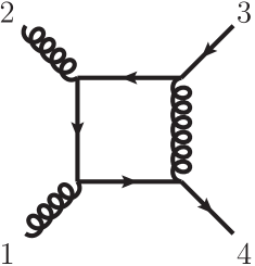
Refer to caption
(a)
Refer to caption
(b)
Figure 8: External fermion box diagrams for (a) the right-turning fermion and (b) the left-turning fermion.
Refer to caption
(a)
Refer to caption
(b)
Figure 9: External fermion box diagrams with internal gluons replaced by scalars.

Next we turn to the case of external fermions. The leading-color contribution to a one-loop amplitude with two external fermions can be decomposed as Bern2g3f

Anf=AnL1Nc2AnR+NfNcAnL,[1/2]+NsNcAnL,[0].superscriptsubscript𝐴𝑛𝑓superscriptsubscript𝐴𝑛𝐿1superscriptsubscript𝑁𝑐2superscriptsubscript𝐴𝑛𝑅subscript𝑁𝑓subscript𝑁𝑐superscriptsubscript𝐴𝑛𝐿delimited-[]12subscript𝑁𝑠subscript𝑁𝑐superscriptsubscript𝐴𝑛𝐿delimited-[]0\displaystyle A_{n}^{f}=A_{n}^{L}-\frac{1}{N_{c}^{2}}A_{n}^{R}+\frac{N_{f}}{N_{c}}A_{n}^{L,[1/2]}+\frac{N_{s}}{N_{c}}A_{n}^{L,[0]}. (154)

Only amplitudes with adjacent external fermions contribute at leading color. AnLsuperscriptsubscript𝐴𝑛𝐿A_{n}^{L} is the “left-turning” fermion piece where the fermion follows the shortest path through the loop (see Fig. 8b), while for AnRsuperscriptsubscript𝐴𝑛𝑅A_{n}^{R} the fermion follows the longest path (Fig. 8a). AnL,[1/2]superscriptsubscript𝐴𝑛𝐿delimited-[]12A_{n}^{L,[1/2]} and AnL,[0]superscriptsubscript𝐴𝑛𝐿delimited-[]0A_{n}^{L,[0]} have, respectively, a fermion and scalar loop and are therefore proportional to the number of each. We focus on the left- and right-turning pieces and calculate the cuts in Fig. 8. (For our sample helicity arrangement to follow, AnL,[1/2]superscriptsubscript𝐴𝑛𝐿delimited-[]12A_{n}^{L,[1/2]} and AnL,[0]superscriptsubscript𝐴𝑛𝐿delimited-[]0A_{n}^{L,[0]} happen to vanish.)

Once again the extra spin states of six dimensions must be treated with a state-sum reduction procedure. Fortunately our findings in section V give us good physical intuition hinting at the appropriate procedure. Fermions have additional states, but since we calculate with a six-dimensional chiral quark with only two states, no reduction procedure is necessary. For gluons, we interpret the extra-dimensional polarization states as scalars and subtract twice the contribution of an amplitude with a scalar loop replacing the gluon loop. The natural generalization then is to replace any internal gluons by scalars, even if they do not comprise the entire loop, and subtract twice the contribution of this diagram from a diagram with internal gluons. For example, cuts from the diagrams in Fig. 9 should be subtracted from their corresponding diagrams in Fig. 8 to reduce to the FDH scheme.

For a more rigorous motivation, we again appeal to the Feynman rules. The dimensional dependence for Feynman loop diagrams involving external fermions arises through a contraction of gamma matrices. If we isolate the terms with dimensional dependence, we find them to differ only by a factor of D𝐷D from equivalent diagrams with all internal gluons replaced by scalars. We can therefore summarize our procedure as

CFDH=C(6)2Cscalar.superscript𝐶FDHsuperscript𝐶62superscript𝐶scalar\displaystyle C^{\mathrm{FDH}}=C^{(6)}-2C^{\mathrm{scalar}}. (155)

VI.1 Right-turning A4(1)(1+,2,3q¯,4q+)superscriptsubscript𝐴41superscript1superscript2superscriptsubscript3¯𝑞superscriptsubscript4𝑞A_{4}^{(1)}(1^{+},2^{-},3_{\bar{q}}^{-},4_{q}^{+})

As an example we calculate A4(1)(1+,2,3q¯,4q+)superscriptsubscript𝐴41superscript1superscript2superscriptsubscript3¯𝑞superscriptsubscript4𝑞A_{4}^{(1)}(1^{+},2^{-},3_{\bar{q}}^{-},4_{q}^{+}) for both the right-turning and left-turning configurations. For the right-turning, we require the two-chiral-quark two-gluon tree amplitude (27) to sew four-point amplitudes across the s23subscript𝑠23s_{23} channel. We also need the four-chiral-quark tree amplitude with a gluon propagator444If we wanted to compute a four-dimensional tree amplitude using this, we would need to reduce the state-sum by subtracting two times the diagrams with a scalar propagator replacing the gluon propagator. The six-dimensional chirality of the external quarks is not important in four dimensions since each chirality separately carries both helicity states of the four-dimensional quark.,

A4(0);g(1aq,2bq,3cq,4dq)=is13s12s231a2b3c4d,superscriptsubscript𝐴40𝑔superscriptsubscript1𝑎𝑞superscriptsubscript2𝑏𝑞superscriptsubscript3𝑐𝑞superscriptsubscript4𝑑𝑞𝑖subscript𝑠13subscript𝑠12subscript𝑠23delimited-⟨⟩subscript1𝑎subscript2𝑏subscript3𝑐subscript4𝑑\displaystyle A_{4}^{(0);g}(1_{a}^{q},2_{b}^{q},3_{c}^{q},4_{d}^{q})=-i\frac{s_{13}}{s_{12}s_{23}}\langle 1_{a}2_{b}3_{c}4_{d}\rangle, (156)

for sewing across the s12subscript𝑠12s_{12} channel. Using these in our normal procedure, we find the six-dimensional coefficients,

C4[0],6D=12A4(0)s122s23s13,C4[4],6D=0,C3;12[0],6D=12A4(0)(s12s12s23s13),C3;12[2],6D=A4(0)(2+s13s23s23s13),C3;23[0],6D=12A4(0)s12s23s13,C3;23[2],6D=A4(0)s12s13,C3;34[0],6D=12A4(0)(s12+s12s23s13),C3;34[2],6D=A4(0)(2+s13s23+s23s13),C3;41[0],6D=12A4(0)s12s23s13,C3;41[2],6D=A4(0)s12s13,C2;12[0],6D=A4(0),C2;12[2],6D=0,C2;23[0],6D=0,C2;23[2],6D=0,superscriptsubscript𝐶4delimited-[]06𝐷12superscriptsubscript𝐴40superscriptsubscript𝑠122subscript𝑠23subscript𝑠13superscriptsubscript𝐶4delimited-[]46𝐷0superscriptsubscript𝐶312delimited-[]06𝐷12superscriptsubscript𝐴40subscript𝑠12subscript𝑠12subscript𝑠23subscript𝑠13superscriptsubscript𝐶312delimited-[]26𝐷superscriptsubscript𝐴402subscript𝑠13subscript𝑠23subscript𝑠23subscript𝑠13superscriptsubscript𝐶323delimited-[]06𝐷12superscriptsubscript𝐴40subscript𝑠12subscript𝑠23subscript𝑠13superscriptsubscript𝐶323delimited-[]26𝐷superscriptsubscript𝐴40subscript𝑠12subscript𝑠13superscriptsubscript𝐶334delimited-[]06𝐷12superscriptsubscript𝐴40subscript𝑠12subscript𝑠12subscript𝑠23subscript𝑠13superscriptsubscript𝐶334delimited-[]26𝐷superscriptsubscript𝐴402subscript𝑠13subscript𝑠23subscript𝑠23subscript𝑠13superscriptsubscript𝐶341delimited-[]06𝐷12superscriptsubscript𝐴40subscript𝑠12subscript𝑠23subscript𝑠13superscriptsubscript𝐶341delimited-[]26𝐷superscriptsubscript𝐴40subscript𝑠12subscript𝑠13superscriptsubscript𝐶212delimited-[]06𝐷superscriptsubscript𝐴40superscriptsubscript𝐶212delimited-[]26𝐷0superscriptsubscript𝐶223delimited-[]06𝐷0superscriptsubscript𝐶223delimited-[]26𝐷0\displaystyle\begin{array}[]{ll}C_{4}^{[0],6D}=\frac{1}{2}A_{4}^{(0)}\frac{s_{12}^{2}s_{23}}{s_{13}},&C_{4}^{[4],6D}=0,\\ C_{3;12}^{[0],6D}=\frac{1}{2}A_{4}^{(0)}\left(s_{12}-\frac{s_{12}s_{23}}{s_{13}}\right),&C_{3;12}^{[2],6D}=A_{4}^{(0)}\left(2+\frac{s_{13}}{s_{23}}-\frac{s_{23}}{s_{13}}\right),\\ C_{3;23}^{[0],6D}=\frac{1}{2}A_{4}^{(0)}\frac{s_{12}s_{23}}{s_{13}},&C_{3;23}^{[2],6D}=-A_{4}^{(0)}\frac{s_{12}}{s_{13}},\\ C_{3;34}^{[0],6D}=-\frac{1}{2}A_{4}^{(0)}\left(s_{12}+\frac{s_{12}s_{23}}{s_{13}}\right),&C_{3;34}^{[2],6D}=-A_{4}^{(0)}\left(2+\frac{s_{13}}{s_{23}}+\frac{s_{23}}{s_{13}}\right),\\ C_{3;41}^{[0],6D}=\frac{1}{2}A_{4}^{(0)}\frac{s_{12}s_{23}}{s_{13}},&C_{3;41}^{[2],6D}=-A_{4}^{(0)}\frac{s_{12}}{s_{13}},\\ C_{2;12}^{[0],6D}=-A_{4}^{(0)},&C_{2;12}^{[2],6D}=0,\\ C_{2;23}^{[0],6D}=0,&C_{2;23}^{[2],6D}=0,\end{array} (164)

where

A4(0)superscriptsubscript𝐴40\displaystyle A_{4}^{(0)} =i2 332 41 22 33 44 1.absent𝑖superscriptdelimited-⟨⟩233delimited-⟨⟩24delimited-⟨⟩12delimited-⟨⟩23delimited-⟨⟩34delimited-⟨⟩41\displaystyle=i\frac{\langle 2\,3\rangle^{3}\langle 2\,4\rangle}{\langle 1\,2\rangle\langle 2\,3\rangle\langle 3\,4\rangle\langle 4\,1\rangle}. (165)

To perform the state-sum reduction, our required tree amplitudes are the two-chiral-quark two-anti-chiral-quark amplitude with a scalar propagator (with adjacent chiral quarks) and the chiral-quark anti-chiral-quark scalar gluon amplitude,

A4(0);s(1aq,2bq,3c˙q,4d˙q)superscriptsubscript𝐴40𝑠superscriptsubscript1𝑎𝑞superscriptsubscript2𝑏𝑞superscriptsubscript3˙𝑐𝑞superscriptsubscript4˙𝑑𝑞\displaystyle A_{4}^{(0);s}(1_{a}^{q},2_{b}^{q},3_{\dot{c}}^{q},4_{\dot{d}}^{q}) =i2s231a|4d˙]2b|3c˙],\displaystyle=-\frac{i}{2s_{23}}\langle 1_{a}|4_{\dot{d}}]\langle 2_{b}|3_{\dot{c}}],
A4(0)(1aa˙g,2bq,3s,4d˙q)superscriptsubscript𝐴40superscriptsubscript1𝑎˙𝑎𝑔superscriptsubscript2𝑏𝑞superscript3𝑠superscriptsubscript4˙𝑑𝑞\displaystyle A_{4}^{(0)}(1_{a\dot{a}}^{g},2_{b}^{q},3^{s},4_{\dot{d}}^{q}) =i42s12s231a2b3c3c[1a˙3c˙3c˙4d˙],absent𝑖42subscript𝑠12subscript𝑠23delimited-⟨⟩subscript1𝑎subscript2𝑏subscript3𝑐superscript3𝑐delimited-[]subscript1˙𝑎superscript3˙𝑐subscript3˙𝑐subscript4˙𝑑\displaystyle=-\frac{i}{4\sqrt{2}s_{12}s_{23}}\langle 1_{a}2_{b}3_{c}3^{c}\rangle[1_{\dot{a}}3^{\dot{c}}3_{\dot{c}}4_{\dot{d}}], (166)

as computed from Feynman diagrams. The coefficients for diagrams with internal gluons replaced by scalars are

C4[0]=0,C4[4]=0,C3;12[0]=0,C3;12[2]=14A4(0)(2+s13s23s23s13),C3;23[0]=0,C3;23[2]=14A4(0)s12s13,C3;34[0]=0,C3;34[2]=14A4(0)(2+s13s23+s23s13),C3;41[0]=0,C3;41[2]=14A4(0)s12s13,C2;12[0]=14A4(0),C2;12[2]=0,C2;23[0]=0,C2;23[2]=0.superscriptsubscript𝐶4delimited-[]00superscriptsubscript𝐶4delimited-[]40superscriptsubscript𝐶312delimited-[]00superscriptsubscript𝐶312delimited-[]214superscriptsubscript𝐴402subscript𝑠13subscript𝑠23subscript𝑠23subscript𝑠13superscriptsubscript𝐶323delimited-[]00superscriptsubscript𝐶323delimited-[]214superscriptsubscript𝐴40subscript𝑠12subscript𝑠13superscriptsubscript𝐶334delimited-[]00superscriptsubscript𝐶334delimited-[]214superscriptsubscript𝐴402subscript𝑠13subscript𝑠23subscript𝑠23subscript𝑠13superscriptsubscript𝐶341delimited-[]00superscriptsubscript𝐶341delimited-[]214superscriptsubscript𝐴40subscript𝑠12subscript𝑠13superscriptsubscript𝐶212delimited-[]014superscriptsubscript𝐴40superscriptsubscript𝐶212delimited-[]20superscriptsubscript𝐶223delimited-[]00superscriptsubscript𝐶223delimited-[]20\displaystyle\begin{array}[]{ll}C_{4}^{[0]}=0,&C_{4}^{[4]}=0,\\ C_{3;12}^{[0]}=0,&C_{3;12}^{[2]}=\frac{1}{4}A_{4}^{(0)}\left(2+\frac{s_{13}}{s_{23}}-\frac{s_{23}}{s_{13}}\right),\\ C_{3;23}^{[0]}=0,&C_{3;23}^{[2]}=-\frac{1}{4}A_{4}^{(0)}\frac{s_{12}}{s_{13}},\\ C_{3;34}^{[0]}=0,&C_{3;34}^{[2]}=-\frac{1}{4}A_{4}^{(0)}\left(2+\frac{s_{13}}{s_{23}}+\frac{s_{23}}{s_{13}}\right),\\ C_{3;41}^{[0]}=0,&C_{3;41}^{[2]}=-\frac{1}{4}A_{4}^{(0)}\frac{s_{12}}{s_{13}},\\ C_{2;12}^{[0]}=\frac{1}{4}A_{4}^{(0)},&C_{2;12}^{[2]}=0,\\ C_{2;23}^{[0]}=0,&C_{2;23}^{[2]}=0.\end{array} (174)

After utilizing our state-sum reduction procedure and combining terms with invariants in the same channel, we finally have,

C4[0]=12A4(0)s122s23s13,C4[4]=0,C3;s12[0]=A4(0)s12s23s13,C3;s12[2]=A4(0)s23s13,C3;s23[0]=A4(0)s12s23s13,C3;s23[2]=A4(0)s12s13,C2;12[0]=32A4(0),C2;12[2]=0,C2;23[0]=0,C2;23[2]=0,superscriptsubscript𝐶4delimited-[]012superscriptsubscript𝐴40superscriptsubscript𝑠122subscript𝑠23subscript𝑠13superscriptsubscript𝐶4delimited-[]40superscriptsubscript𝐶3subscript𝑠12delimited-[]0superscriptsubscript𝐴40subscript𝑠12subscript𝑠23subscript𝑠13superscriptsubscript𝐶3subscript𝑠12delimited-[]2superscriptsubscript𝐴40subscript𝑠23subscript𝑠13superscriptsubscript𝐶3subscript𝑠23delimited-[]0superscriptsubscript𝐴40subscript𝑠12subscript𝑠23subscript𝑠13superscriptsubscript𝐶3subscript𝑠23delimited-[]2superscriptsubscript𝐴40subscript𝑠12subscript𝑠13superscriptsubscript𝐶212delimited-[]032superscriptsubscript𝐴40superscriptsubscript𝐶212delimited-[]20superscriptsubscript𝐶223delimited-[]00superscriptsubscript𝐶223delimited-[]20\displaystyle\begin{array}[]{ll}C_{4}^{[0]}=\frac{1}{2}A_{4}^{(0)}\frac{s_{12}^{2}s_{23}}{s_{13}},&C_{4}^{[4]}=0,\\ C_{3;s_{12}}^{[0]}=-A_{4}^{(0)}\frac{s_{12}s_{23}}{s_{13}},&C_{3;s_{12}}^{[2]}=-A_{4}^{(0)}\frac{s_{23}}{s_{13}},\\ C_{3;s_{23}}^{[0]}=A_{4}^{(0)}\frac{s_{12}s_{23}}{s_{13}},&C_{3;s_{23}}^{[2]}=-A_{4}^{(0)}\frac{s_{12}}{s_{13}},\\ C_{2;12}^{[0]}=-\frac{3}{2}A_{4}^{(0)},&C_{2;12}^{[2]}=0,\\ C_{2;23}^{[0]}=0,&C_{2;23}^{[2]}=0,\end{array} (180)

in agreement with the previously known result KunsztResults .

VI.2 Left-turning A4(1)(1+,2,3q¯,4q+)superscriptsubscript𝐴41superscript1superscript2superscriptsubscript3¯𝑞superscriptsubscript4𝑞A_{4}^{(1)}(1^{+},2^{-},3_{\bar{q}}^{-},4_{q}^{+})

For the left-turning diagram (Fig. 8b), the only new tree amplitude that we require is the two-chiral-quark two-scalar amplitude,

A4(0)(1s,2s,3cq,4dq)=i(s13s23)4s12s231a1a3c4d.superscriptsubscript𝐴40superscript1𝑠superscript2𝑠superscriptsubscript3𝑐𝑞superscriptsubscript4𝑑𝑞𝑖subscript𝑠13subscript𝑠234subscript𝑠12subscript𝑠23delimited-⟨⟩subscript1𝑎superscript1𝑎subscript3𝑐subscript4𝑑\displaystyle A_{4}^{(0)}(1^{s},2^{s},3_{c}^{q},4_{d}^{q})=\frac{i(s_{13}-s_{23})}{4s_{12}s_{23}}\langle 1_{a}1^{a}3_{c}4_{d}\rangle. (181)

Proceeding as usual, we find for our coefficients,

C4[0]=A4(0)(s12s23+12s122s23s13),C4[4]=0,C3;s12[0]=A4(0)s12s23s13,C3;s12[2]=A4(0)s23s13,C3;s23[0]=A4(0)s12s23s13,C3;s23[2]=A4(0)s12s13,C2;12[0]=32A4(0),C2;12[2]=0,C2;23[0]=0,C2;23[2]=0,superscriptsubscript𝐶4delimited-[]0superscriptsubscript𝐴40subscript𝑠12subscript𝑠2312superscriptsubscript𝑠122subscript𝑠23subscript𝑠13superscriptsubscript𝐶4delimited-[]40superscriptsubscript𝐶3subscript𝑠12delimited-[]0superscriptsubscript𝐴40subscript𝑠12subscript𝑠23subscript𝑠13superscriptsubscript𝐶3subscript𝑠12delimited-[]2superscriptsubscript𝐴40subscript𝑠23subscript𝑠13superscriptsubscript𝐶3subscript𝑠23delimited-[]0superscriptsubscript𝐴40subscript𝑠12subscript𝑠23subscript𝑠13superscriptsubscript𝐶3subscript𝑠23delimited-[]2superscriptsubscript𝐴40subscript𝑠12subscript𝑠13superscriptsubscript𝐶212delimited-[]032superscriptsubscript𝐴40superscriptsubscript𝐶212delimited-[]20superscriptsubscript𝐶223delimited-[]00superscriptsubscript𝐶223delimited-[]20\displaystyle\begin{array}[]{ll}C_{4}^{[0]}=-A_{4}^{(0)}\left(s_{12}s_{23}+\frac{1}{2}\frac{s_{12}^{2}s_{23}}{s_{13}}\right),&C_{4}^{[4]}=0,\\ C_{3;s_{12}}^{[0]}=A_{4}^{(0)}\frac{s_{12}s_{23}}{s_{13}},&C_{3;s_{12}}^{[2]}=A_{4}^{(0)}\frac{s_{23}}{s_{13}},\\ C_{3;s_{23}}^{[0]}=-A_{4}^{(0)}\frac{s_{12}s_{23}}{s_{13}},&C_{3;s_{23}}^{[2]}=A_{4}^{(0)}\frac{s_{12}}{s_{13}},\\ C_{2;12}^{[0]}=-\frac{3}{2}A_{4}^{(0)},&C_{2;12}^{[2]}=0,\\ C_{2;23}^{[0]}=0,&C_{2;23}^{[2]}=0,\end{array} (187)

once again in agreement with ref. KunsztResults .

VII HIGGS TO PARTONS PROCESSES: A3(1)(H,1+,2+,3+)subscriptsuperscript𝐴13𝐻superscript1superscript2superscript3A^{(1)}_{3}(H,1^{+},2^{+},3^{+})

An important process for the Higgs boson search is production via the strong interaction. In the Standard Model, the Higgs couples to two gluons via a heavy-quark loop GeorgiGlashow . The dominant contribution is from the top quark; contributions from other quarks are suppressed by at least a factor of O(mb2/mt2)𝑂superscriptsubscript𝑚𝑏2superscriptsubscript𝑚𝑡2O(m_{b}^{2}/m_{t}^{2}) where mbsubscript𝑚𝑏m_{b} is the mass of the bottom quark and mtsubscript𝑚𝑡m_{t} is the mass of the top.

Computations that keep explicit dependence on mtsubscript𝑚𝑡m_{t} can be difficult, especially at NLO since they involve two-loop amplitudes. Fortunately in the large-mtsubscript𝑚𝑡m_{t} limit, where the mass of the Higgs mHsubscript𝑚𝐻m_{H} is smaller than the threshold for top-quark pair production, mH<2mtsubscript𝑚𝐻2subscript𝑚𝑡m_{H}<2m_{t}, computations are greatly simplified by letting mtsubscript𝑚𝑡m_{t}\rightarrow\infty Wilczek ; Djouadi ; Dawson . Accurate approximations (to within 10%percent1010\% of the Higgs-mass range at the LHC) of NLO QCD corrections can be found by finding the NLO QCD correction factor, KNLOσNLO/σLOsuperscript𝐾𝑁𝐿𝑂superscript𝜎𝑁𝐿𝑂superscript𝜎𝐿𝑂K^{NLO}\equiv\sigma^{NLO}/\sigma^{LO} in the limit mtsubscript𝑚𝑡m_{t}\rightarrow\infty, then multiplying by the exact leading-order cross section Kramer . The approximation is valid for multi-jet processes provided the transverse momentum of each jet is less than mtsubscript𝑚𝑡m_{t} DelDucaKilgore .

Taking the limit mtsubscript𝑚𝑡m_{t}\rightarrow\infty allows us to use an effective Lagrangian to express the coupling of the Higgs to gluons Wilczek ,

Hint=C2HtrGμνGμν.subscriptsuperscriptint𝐻𝐶2𝐻trsubscript𝐺𝜇𝜈superscript𝐺𝜇𝜈\displaystyle\mathcal{L}^{\mathrm{int}}_{H}=\frac{C}{2}H\,\mathrm{tr}\,G_{\mu\nu}G^{\mu\nu}. (188)

This reduces two-loop calculations at NLO to one-loop calculations. The Higgs two-gluon color-ordered vertex is

2i(ημ1μ2k1k2k1μ2k2μ1),2𝑖superscript𝜂subscript𝜇1subscript𝜇2subscript𝑘1subscript𝑘2superscriptsubscript𝑘1subscript𝜇2superscriptsubscript𝑘2subscript𝜇1\displaystyle-2i(\eta^{\mu_{1}\mu_{2}}k_{1}\cdot k_{2}-k_{1}^{\mu_{2}}k_{2}^{\mu_{1}}), (189)

which gives the six-dimensional helicity tree amplitude,

A2(0)(H,1aa˙,2bb˙)=i1a|2b˙]2b|1a˙].\displaystyle A_{2}^{(0)}(H,1_{a\dot{a}},2_{b\dot{b}})=i\langle 1_{a}|2_{\dot{b}}]\langle 2_{b}|1_{\dot{a}}]. (190)

The Higgs three-gluon vertex factor is

i2(ημ1μ2(k1k2)μ3+ημ2μ3(k2k3)μ1+ημ3μ1(k3k1)μ2),𝑖2superscript𝜂subscript𝜇1subscript𝜇2superscriptsubscript𝑘1subscript𝑘2subscript𝜇3superscript𝜂subscript𝜇2subscript𝜇3superscriptsubscript𝑘2subscript𝑘3subscript𝜇1superscript𝜂subscript𝜇3subscript𝜇1superscriptsubscript𝑘3subscript𝑘1subscript𝜇2\displaystyle-i\sqrt{2}(\eta^{\mu_{1}\mu_{2}}(k_{1}-k_{2})^{\mu_{3}}+\eta^{\mu_{2}\mu_{3}}(k_{2}-k_{3})^{\mu_{1}}+\eta^{\mu_{3}\mu_{1}}(k_{3}-k_{1})^{\mu_{2}}), (191)

which, when combined with other relevant Feynman diagrams, gives the tree amplitude,

A3(0)(H,1aa˙,2bb˙,3cc˙)=is12s232s132superscriptsubscript𝐴30𝐻subscript1𝑎˙𝑎subscript2𝑏˙𝑏subscript3𝑐˙𝑐𝑖subscript𝑠12superscriptsubscript𝑠232superscriptsubscript𝑠132\displaystyle A_{3}^{(0)}(H,1_{a\dot{a}},2_{b\dot{b}},3_{c\dot{c}})=\frac{-i}{s_{12}s_{23}^{2}s_{13}^{2}} {(s12mH2+s13s23)1a|/k3|2b[1a˙|/k3|2b˙]3c|/k2/k1|3c˙]delimited-{]conditionalsubscript𝑠12superscriptsubscript𝑚𝐻2subscript𝑠13subscript𝑠23quantum-operator-productsubscript1𝑎subscript/k3subscript2𝑏delimited-[]subscript1˙𝑎subscript/k3subscript2˙𝑏brasubscript3𝑐subscript/k2subscript/k1subscript3˙𝑐\displaystyle\left\{(s_{12}m_{H}^{2}+s_{13}s_{23})\langle 1_{a}|{\raise 0.97221pt\hbox to5.52084pt{\hss/\hss}\hbox to0.0pt{\hss$k$}}_{3}|2_{b}\rangle[1_{\dot{a}}|{\raise 0.97221pt\hbox to5.52084pt{\hss/\hss}\hbox to0.0pt{\hss$k$}}_{3}|2_{\dot{b}}]\langle 3_{c}|{\raise 0.97221pt\hbox to5.52084pt{\hss/\hss}\hbox to0.0pt{\hss$k$}}_{2}{\raise 0.97221pt\hbox to5.52084pt{\hss/\hss}\hbox to0.0pt{\hss$k$}}_{1}|3_{\dot{c}}]\right.
s23(s13mH2+s12s23)1a|3c˙]3c|1a˙]2b|/k1/k3|2b˙]\displaystyle-s_{23}(s_{13}m_{H}^{2}+s_{12}s_{23})\langle 1_{a}|3_{\dot{c}}]\langle 3_{c}|1_{\dot{a}}]\langle 2_{b}|{\raise 0.97221pt\hbox to5.52084pt{\hss/\hss}\hbox to0.0pt{\hss$k$}}_{1}{\raise 0.97221pt\hbox to5.52084pt{\hss/\hss}\hbox to0.0pt{\hss$k$}}_{3}|2_{\dot{b}}]
+s13(s23mH2+s12s13)2b|3c˙]3c|2b˙]1a|/k2/k3|1a˙]\displaystyle+s_{13}(s_{23}m_{H}^{2}+s_{12}s_{13})\langle 2_{b}|3_{\dot{c}}]\langle 3_{c}|2_{\dot{b}}]\langle 1_{a}|{\raise 0.97221pt\hbox to5.52084pt{\hss/\hss}\hbox to0.0pt{\hss$k$}}_{2}{\raise 0.97221pt\hbox to5.52084pt{\hss/\hss}\hbox to0.0pt{\hss$k$}}_{3}|1_{\dot{a}}]
s121a|/k2/k3|1a˙]2b|/k1/k3|2b˙]3c|/k2/k1|3c˙]}.\displaystyle\left.-s_{12}\langle 1_{a}|{\raise 0.97221pt\hbox to5.52084pt{\hss/\hss}\hbox to0.0pt{\hss$k$}}_{2}{\raise 0.97221pt\hbox to5.52084pt{\hss/\hss}\hbox to0.0pt{\hss$k$}}_{3}|1_{\dot{a}}]\langle 2_{b}|{\raise 0.97221pt\hbox to5.52084pt{\hss/\hss}\hbox to0.0pt{\hss$k$}}_{1}{\raise 0.97221pt\hbox to5.52084pt{\hss/\hss}\hbox to0.0pt{\hss$k$}}_{3}|2_{\dot{b}}]\langle 3_{c}|{\raise 0.97221pt\hbox to5.52084pt{\hss/\hss}\hbox to0.0pt{\hss$k$}}_{2}{\raise 0.97221pt\hbox to5.52084pt{\hss/\hss}\hbox to0.0pt{\hss$k$}}_{1}|3_{\dot{c}}]\right\}. (192)

We use these to calculate A3(1)(H,1+,2+,3+)subscriptsuperscript𝐴13𝐻superscript1superscript2superscript3A^{(1)}_{3}(H,1^{+},2^{+},3^{+}), first given in ref. Schmidt .

VII.1 Momentum solutions
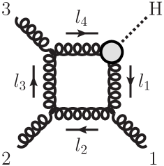
Refer to caption

Figure 10: A possible box diagram for A3(1)(H,1+,2+,3+)subscriptsuperscript𝐴13𝐻superscript1superscript2superscript3A^{(1)}_{3}(H,1^{+},2^{+},3^{+}) using the effective coupling of the Higgs to two gluons. We denote this cut with ordering “123H”.

Momentum solutions can be a bit more complicated with a massive leg. We give explicit forms in line with those in section IV. For the box in Fig. 10, we use

l¯2=c±λ1λ~21c±mm~s12λ2λ~1,subscript¯𝑙2subscript𝑐plus-or-minussubscript𝜆1subscript~𝜆21subscript𝑐plus-or-minus𝑚~𝑚subscript𝑠12subscript𝜆2subscript~𝜆1\displaystyle\bar{l}_{2}=c_{\pm}\lambda_{1}\tilde{\lambda}_{2}-\frac{1}{c_{\pm}}\frac{m\tilde{m}}{s_{12}}\lambda_{2}\tilde{\lambda}_{1}, (193)

where

c±=2 321 3(1±1+4mm~s13s12s23).subscript𝑐plus-or-minusdelimited-⟨⟩232delimited-⟨⟩13plus-or-minus114𝑚~𝑚subscript𝑠13subscript𝑠12subscript𝑠23\displaystyle c_{\pm}=\frac{\langle 2\,3\rangle}{2\langle 1\,3\rangle}\left(1\pm\sqrt{1+\frac{4m\tilde{m}s_{13}}{s_{12}s_{23}}}\right). (194)

The triple-cut solution for cutting propagators l1subscript𝑙1l_{1}, l2subscript𝑙2l_{2} and l3subscript𝑙3l_{3} can be found by letting c±tsubscript𝑐plus-or-minus𝑡c_{\pm}\rightarrow t. To cut l1subscript𝑙1l_{1}, l3subscript𝑙3l_{3} and l4subscript𝑙4l_{4}, we use

l¯4=mH2γ3Hλ3λ~3+tλ3λ~Hmm~tγ3HλHλ~3,subscript¯𝑙4superscriptsubscript𝑚𝐻2subscript𝛾3𝐻subscript𝜆3subscript~𝜆3𝑡subscript𝜆3superscriptsubscript~𝜆𝐻𝑚~𝑚𝑡subscript𝛾3𝐻superscriptsubscript𝜆𝐻subscript~𝜆3\displaystyle\bar{l}_{4}=\frac{m_{H}^{2}}{\gamma_{3H}}\lambda_{3}\tilde{\lambda}_{3}+t\lambda_{3}\tilde{\lambda}_{H}^{\flat}-\frac{m\tilde{m}}{t\gamma_{3H}}\lambda_{H}^{\flat}\tilde{\lambda}_{3}, (195)

where

KHsuperscriptsubscript𝐾𝐻\displaystyle K_{H}^{\flat} =kHmH2γ3Hk3,absentsubscript𝑘𝐻superscriptsubscript𝑚𝐻2subscript𝛾3𝐻subscript𝑘3\displaystyle=k_{H}-\frac{m_{H}^{2}}{\gamma_{3H}}k_{3},
γ3Hsubscript𝛾3𝐻\displaystyle\gamma_{3H} =2kHk3absent2subscript𝑘𝐻subscript𝑘3\displaystyle=2k_{H}\cdot k_{3}
=s13s23.absentsubscript𝑠13subscript𝑠23\displaystyle=-s_{13}-s_{23}. (196)

This allows us to set

μ=λH,μ~=λ~3t,λ=λ3,λ~=mH2γ3Hλ~3+tλ~H,formulae-sequence𝜇superscriptsubscript𝜆𝐻formulae-sequence~𝜇subscript~𝜆3𝑡formulae-sequence𝜆subscript𝜆3~𝜆superscriptsubscript𝑚𝐻2subscript𝛾3𝐻subscript~𝜆3𝑡superscriptsubscript~𝜆𝐻\displaystyle\mu=\lambda_{H}^{\flat},\hskip 22.76219pt\tilde{\mu}=\frac{\tilde{\lambda}_{3}}{t},\hskip 22.76219pt\lambda=\lambda_{3},\hskip 22.76219pt\tilde{\lambda}=\frac{m_{H}^{2}}{\gamma_{3H}}\tilde{\lambda}_{3}+t\tilde{\lambda}_{H}^{\flat},
κ3H=subscript𝜅3𝐻absent\displaystyle\kappa_{3H}= m3λH,κ~3H=m~[3λH],κ3H=m[3λH],κ~3H=m~3λH.formulae-sequence𝑚delimited-⟨⟩3superscriptsubscript𝜆𝐻subscript~𝜅3𝐻~𝑚delimited-[]3superscriptsubscript𝜆𝐻formulae-sequencesuperscriptsubscript𝜅3𝐻𝑚delimited-[]3superscriptsubscript𝜆𝐻superscriptsubscript~𝜅3𝐻~𝑚delimited-⟨⟩3superscriptsubscript𝜆𝐻\displaystyle\frac{m}{\langle 3\lambda_{H}^{\flat}\rangle},\hskip 22.76219pt\tilde{\kappa}_{3H}=\frac{\tilde{m}}{[3\lambda_{H}^{\flat}]},\hskip 22.76219pt\kappa_{3H}^{\prime}=\frac{m}{[3\lambda_{H}^{\flat}]},\hskip 22.76219pt\tilde{\kappa}_{3H}^{\prime}=\frac{\tilde{m}}{\langle 3\lambda_{H}^{\flat}\rangle}. (197)

Making similar associations for l1subscript𝑙1l_{1} and l3subscript𝑙3l_{3} through the use of momentum conservation allows us to find the necessary spinor products. We find the cut for the conjugate momentum solution by taking tmm~tγ3H𝑡𝑚~𝑚𝑡subscript𝛾3𝐻t\rightarrow-\frac{m\tilde{m}}{t\gamma_{3H}}.

To cut l1subscript𝑙1l_{1} and l3subscript𝑙3l_{3}, we use

l¯1=yλ1λ~1+(1y)λ2λ~2+tλ1λ~2+y(1y)mm~/s12tλ2λ~1,subscript¯𝑙1𝑦subscript𝜆1subscript~𝜆11𝑦subscript𝜆2subscript~𝜆2𝑡subscript𝜆1subscript~𝜆2𝑦1𝑦𝑚~𝑚subscript𝑠12𝑡subscript𝜆2subscript~𝜆1\displaystyle\bar{l}_{1}=y\lambda_{1}\tilde{\lambda}_{1}+(1-y)\lambda_{2}\tilde{\lambda}_{2}+t\lambda_{1}\tilde{\lambda}_{2}+\frac{y(1-y)-m\tilde{m}/s_{12}}{t}\lambda_{2}\tilde{\lambda}_{1}, (198)

whereas to cut l1subscript𝑙1l_{1} and l4subscript𝑙4l_{4} we use

l¯4=yλHλ~H+mH2γ¯(1y)λ3λ~3+tλHλ~3+y(1y)mH2mm~tγ¯λ3λ~H,subscript¯𝑙4𝑦superscriptsubscript𝜆𝐻superscriptsubscript~𝜆𝐻superscriptsubscript𝑚𝐻2¯𝛾1𝑦subscript𝜆3subscript~𝜆3𝑡superscriptsubscript𝜆𝐻subscript~𝜆3𝑦1𝑦superscriptsubscript𝑚𝐻2𝑚~𝑚𝑡¯𝛾subscript𝜆3superscriptsubscript~𝜆𝐻\displaystyle\bar{l}_{4}=y\lambda_{H}^{\flat}\tilde{\lambda}_{H}^{\flat}+\frac{m_{H}^{2}}{\bar{\gamma}}(1-y)\lambda_{3}\tilde{\lambda}_{3}+t\lambda_{H}^{\flat}\tilde{\lambda}_{3}+\frac{y(1-y)m_{H}^{2}-m\tilde{m}}{t\bar{\gamma}}\lambda_{3}\tilde{\lambda}_{H}^{\flat}, (199)

where

KH=kHmH2γ¯k3,γ¯=s13s23.formulae-sequencesuperscriptsubscript𝐾𝐻subscript𝑘𝐻superscriptsubscript𝑚𝐻2¯𝛾subscript𝑘3¯𝛾subscript𝑠13subscript𝑠23\displaystyle K_{H}^{\flat}=k_{H}-\frac{m_{H}^{2}}{\bar{\gamma}}k_{3},\hskip 56.9055pt\bar{\gamma}=-s_{13}-s_{23}. (200)

All other cuts can be obtained from permutations of the ones given. It should be noted that the Higgs can attach itself to any gluon line, so there are quite a few more cuts than there are for a four-gluon amplitude. Fortunately many coefficients for our particular helicity arrangement are related through cyclic permutations of the external gluon momenta.

VII.2 Six-dimensional coefficients

We explicitly calculate the box coefficients for Fig. 10. The quadruple cut is given by,

C1234=subscript𝐶1234absent\displaystyle C_{1234}= states(i)2l22l42A4(0)(l1g,1+,2+,l3g)A4(0)(l3g,3+,H,l1g)subscriptstatessuperscript𝑖2superscriptsubscript𝑙22superscriptsubscript𝑙42superscriptsubscript𝐴40superscriptsubscript𝑙1𝑔superscript1superscript2superscriptsubscript𝑙3𝑔superscriptsubscript𝐴40superscriptsubscript𝑙3𝑔superscript3𝐻superscriptsubscript𝑙1𝑔\displaystyle\sum_{\mathrm{states}}(-i)^{2}l_{2}^{2}l_{4}^{2}A_{4}^{(0)}(-l_{1}^{g},1^{+},2^{+},l_{3}^{g})A_{4}^{(0)}(-l_{3}^{g},3^{+},H,l_{1}^{g})
=\displaystyle= 1(l1+k3)4s123(l1)a,11,21,(l3)b[(l1)a˙,11˙,21˙,(l3)b˙]1superscriptsubscript𝑙1subscript𝑘34superscriptsubscript𝑠123superscriptsubscript𝑙1𝑎subscript11subscript21superscriptsubscript𝑙3𝑏superscriptsubscript𝑙1˙𝑎subscript1˙1subscript2˙1superscriptsubscript𝑙3˙𝑏\displaystyle\frac{1}{(l_{1}\!+\!k_{3})^{4}s_{12}^{3}}\langle(-l_{1})^{a},1_{1},2_{1},(l_{3})^{b}\rangle\mathrm{[}(-l_{1})^{\dot{a}},1_{\dot{1}},2_{\dot{1}},(l_{3})^{\dot{b}}\mathrm{]}
×{(l42mH2+s12(l1+k3)2)(l3)b|/l1|31[(l3)b˙|/l1|31˙](l1)a|/k3(/l3)|(l1)a˙]\displaystyle\times\left\{(l_{4}^{2}m_{H}^{2}+s_{12}(l_{1}\!+\!k_{3})^{2})\right.\langle(-l_{3})_{b}|{\raise 0.97221pt\hbox to3.18057pt{\hss/\hss}\hbox to0.0pt{\hss$l$}}_{1}|3_{1}\rangle\mathrm{[}(-l_{3})_{\dot{b}}|{\raise 0.97221pt\hbox to3.18057pt{\hss/\hss}\hbox to0.0pt{\hss$l$}}_{1}|3_{\dot{1}}\mathrm{]}\langle(l_{1})_{a}|{\raise 0.97221pt\hbox to5.52084pt{\hss/\hss}\hbox to0.0pt{\hss$k$}}_{3}(-{\raise 0.97221pt\hbox to3.18057pt{\hss/\hss}\hbox to0.0pt{\hss$l$}}_{3})|(l_{1})_{\dot{a}}]
(l1+k3)2(s12mH2+l42(l1+k3)2)(l3)b|(l1)a˙](l1)a|(l3)b˙]31|(/l3)/l1|31˙]\displaystyle-(l_{1}\!+\!k_{3})^{2}(s_{12}m_{H}^{2}+l_{4}^{2}(l_{1}\!+\!k_{3})^{2})\langle(-l_{3})_{b}|(l_{1})_{\dot{a}}]\langle(l_{1})_{a}|(-l_{3})_{\dot{b}}]\langle 3_{1}|(-{\raise 0.97221pt\hbox to3.18057pt{\hss/\hss}\hbox to0.0pt{\hss$l$}}_{3}){\raise 0.97221pt\hbox to3.18057pt{\hss/\hss}\hbox to0.0pt{\hss$l$}}_{1}|3_{\dot{1}}]
+s12((l1+k3)2mH2+l42s12)31|(l1)a˙](l1)a|31˙](l3)b|/k3/l1|(l3)b˙]\displaystyle+s_{12}((l_{1}\!+\!k_{3})^{2}m_{H}^{2}+l_{4}^{2}s_{12})\langle 3_{1}|(l_{1})_{\dot{a}}]\langle(l_{1})_{a}|3_{\dot{1}}]\langle(-l_{3})_{b}|{\raise 0.97221pt\hbox to5.52084pt{\hss/\hss}\hbox to0.0pt{\hss$k$}}_{3}{\raise 0.97221pt\hbox to3.18057pt{\hss/\hss}\hbox to0.0pt{\hss$l$}}_{1}|(-l_{3})_{\dot{b}}]
l42(l3)b|/k3/l1|(l3)b˙]31|(/l3)/l1|31˙](l1)a|/k3(/l3)|(l1)a˙]}.\displaystyle\left.-l_{4}^{2}\langle(-l_{3})_{b}|{\raise 0.97221pt\hbox to5.52084pt{\hss/\hss}\hbox to0.0pt{\hss$k$}}_{3}{\raise 0.97221pt\hbox to3.18057pt{\hss/\hss}\hbox to0.0pt{\hss$l$}}_{1}|(-l_{3})_{\dot{b}}]\langle 3_{1}|(-{\raise 0.97221pt\hbox to3.18057pt{\hss/\hss}\hbox to0.0pt{\hss$l$}}_{3}){\raise 0.97221pt\hbox to3.18057pt{\hss/\hss}\hbox to0.0pt{\hss$l$}}_{1}|3_{\dot{1}}]\langle(l_{1})_{a}|{\raise 0.97221pt\hbox to5.52084pt{\hss/\hss}\hbox to0.0pt{\hss$k$}}_{3}(-{\raise 0.97221pt\hbox to3.18057pt{\hss/\hss}\hbox to0.0pt{\hss$l$}}_{3})|(l_{1})_{\dot{a}}]\right\}. (201)

After averaging over solutions, this becomes

C1234subscript𝐶1234\displaystyle C_{1234} =11 22 33 1[mm~s12s23mH212s12s23mH4].absent1delimited-⟨⟩12delimited-⟨⟩23delimited-⟨⟩31delimited-[]𝑚~𝑚subscript𝑠12subscript𝑠23superscriptsubscript𝑚𝐻212subscript𝑠12subscript𝑠23superscriptsubscript𝑚𝐻4\displaystyle=\frac{1}{\langle 1\,2\rangle\langle 2\,3\rangle\langle 3\,1\rangle}\left[m\tilde{m}s_{12}s_{23}m_{H}^{2}-\frac{1}{2}s_{12}s_{23}m_{H}^{4}\right]. (202)

We can then identify our scalar box coefficient (we neglect C4[2]superscriptsubscript𝐶4delimited-[]2C_{4}^{[2]} since its integral vanishes) for this cut and use permutations to find it for the other quadruple cuts,

C4;123H[0],6Dsuperscriptsubscript𝐶4123𝐻delimited-[]06𝐷\displaystyle C_{4;123H}^{[0],6D} =i2mH41 22 33 1s12s23,absent𝑖2superscriptsubscript𝑚𝐻4delimited-⟨⟩12delimited-⟨⟩23delimited-⟨⟩31subscript𝑠12subscript𝑠23\displaystyle=-\frac{i}{2}\frac{m_{H}^{4}}{\langle 1\,2\rangle\langle 2\,3\rangle\langle 3\,1\rangle}s_{12}s_{23},
C4;1H23[0],6Dsuperscriptsubscript𝐶41𝐻23delimited-[]06𝐷\displaystyle C_{4;1H23}^{[0],6D} =i2mH41 22 33 1s23s13,absent𝑖2superscriptsubscript𝑚𝐻4delimited-⟨⟩12delimited-⟨⟩23delimited-⟨⟩31subscript𝑠23subscript𝑠13\displaystyle=-\frac{i}{2}\frac{m_{H}^{4}}{\langle 1\,2\rangle\langle 2\,3\rangle\langle 3\,1\rangle}s_{23}s_{13},
C4;12H3[0],6Dsuperscriptsubscript𝐶412𝐻3delimited-[]06𝐷\displaystyle C_{4;12H3}^{[0],6D} =i2mH41 22 33 1s12s13,absent𝑖2superscriptsubscript𝑚𝐻4delimited-⟨⟩12delimited-⟨⟩23delimited-⟨⟩31subscript𝑠12subscript𝑠13\displaystyle=-\frac{i}{2}\frac{m_{H}^{4}}{\langle 1\,2\rangle\langle 2\,3\rangle\langle 3\,1\rangle}s_{12}s_{13}, (203)

where the subscript indicates the cyclic ordering of the external particles. Our remaining coefficients are

C3;123H;12[0],6D=12A3(0)(s13+s23),C3;123H;12[2]=A3(0)s13+s23mH2,C3;123H;23[0],6D=12A3(0)(s12+s13),C3;123H;23[2]=A3(0)s12+s13mH2,C3;12H3;13[0],6D=12A3(0)(s12+s23),C3;12H3;13[2]=A3(0)s12+s23mH2,C3;12H3;12[0],6D=12A3(0)(s13+s23),C3;12H3;12[2]=A3(0)s13+s23mH2,C3;1H23;23[0],6D=12A3(0)(s12+s13),C3;1H23;23[2]=A3(0)s12+s13mH2,C3;1H23;13[0],6D=12A3(0)(s12+s23),C3;1H23;13[2]=A3(0)s12+s23mH2,C3;123H;3H[2],6D=4A3(0)s13s23mH4,C3;12H3;2H[2]=4A3(0)s12s23mH4,C3;1H23;1H[2],6D=4A3(0)s12s13mH4,C2;123H;12[2]=8A3(0)s13s23s12mH4,C2;12H3;13[2],6D=8A3(0)s12s23s13mH4,C2;1H23;23[2],6D=8A3(0)s12s13s23mH4,superscriptsubscript𝐶3123𝐻12delimited-[]06𝐷12superscriptsubscript𝐴30subscript𝑠13subscript𝑠23superscriptsubscript𝐶3123𝐻12delimited-[]2superscriptsubscript𝐴30subscript𝑠13subscript𝑠23superscriptsubscript𝑚𝐻2superscriptsubscript𝐶3123𝐻23delimited-[]06𝐷12superscriptsubscript𝐴30subscript𝑠12subscript𝑠13superscriptsubscript𝐶3123𝐻23delimited-[]2superscriptsubscript𝐴30subscript𝑠12subscript𝑠13superscriptsubscript𝑚𝐻2superscriptsubscript𝐶312𝐻313delimited-[]06𝐷12superscriptsubscript𝐴30subscript𝑠12subscript𝑠23superscriptsubscript𝐶312𝐻313delimited-[]2superscriptsubscript𝐴30subscript𝑠12subscript𝑠23superscriptsubscript𝑚𝐻2superscriptsubscript𝐶312𝐻312delimited-[]06𝐷12superscriptsubscript𝐴30subscript𝑠13subscript𝑠23superscriptsubscript𝐶312𝐻312delimited-[]2superscriptsubscript𝐴30subscript𝑠13subscript𝑠23superscriptsubscript𝑚𝐻2superscriptsubscript𝐶31𝐻2323delimited-[]06𝐷12superscriptsubscript𝐴30subscript𝑠12subscript𝑠13superscriptsubscript𝐶31𝐻2323delimited-[]2superscriptsubscript𝐴30subscript𝑠12subscript𝑠13superscriptsubscript𝑚𝐻2superscriptsubscript𝐶31𝐻2313delimited-[]06𝐷12superscriptsubscript𝐴30subscript𝑠12subscript𝑠23superscriptsubscript𝐶31𝐻2313delimited-[]2superscriptsubscript𝐴30subscript𝑠12subscript𝑠23superscriptsubscript𝑚𝐻2superscriptsubscript𝐶3123𝐻3𝐻delimited-[]26𝐷4superscriptsubscript𝐴30subscript𝑠13subscript𝑠23superscriptsubscript𝑚𝐻4superscriptsubscript𝐶312𝐻32𝐻delimited-[]24superscriptsubscript𝐴30subscript𝑠12subscript𝑠23superscriptsubscript𝑚𝐻4superscriptsubscript𝐶31𝐻231𝐻delimited-[]26𝐷4superscriptsubscript𝐴30subscript𝑠12subscript𝑠13superscriptsubscript𝑚𝐻4superscriptsubscript𝐶2123𝐻12delimited-[]28superscriptsubscript𝐴30subscript𝑠13subscript𝑠23subscript𝑠12superscriptsubscript𝑚𝐻4superscriptsubscript𝐶212𝐻313delimited-[]26𝐷8superscriptsubscript𝐴30subscript𝑠12subscript𝑠23subscript𝑠13superscriptsubscript𝑚𝐻4superscriptsubscript𝐶21𝐻2323delimited-[]26𝐷8superscriptsubscript𝐴30subscript𝑠12subscript𝑠13subscript𝑠23superscriptsubscript𝑚𝐻4\displaystyle\begin{array}[]{ll}C_{3;123H;12}^{[0],6D}=\frac{1}{2}A_{3}^{(0)}(s_{13}+s_{23}),&C_{3;123H;12}^{[2]}=-A_{3}^{(0)}\frac{s_{13}+s_{23}}{m_{H}^{2}},\\ C_{3;123H;23}^{[0],6D}=\frac{1}{2}A_{3}^{(0)}(s_{12}+s_{13}),&C_{3;123H;23}^{[2]}=-A_{3}^{(0)}\frac{s_{12}+s_{13}}{m_{H}^{2}},\\ C_{3;12H3;13}^{[0],6D}=\frac{1}{2}A_{3}^{(0)}(s_{12}+s_{23}),&C_{3;12H3;13}^{[2]}=-A_{3}^{(0)}\frac{s_{12}+s_{23}}{m_{H}^{2}},\\ C_{3;12H3;12}^{[0],6D}=\frac{1}{2}A_{3}^{(0)}(s_{13}+s_{23}),&C_{3;12H3;12}^{[2]}=-A_{3}^{(0)}\frac{s_{13}+s_{23}}{m_{H}^{2}},\\ C_{3;1H23;23}^{[0],6D}=\frac{1}{2}A_{3}^{(0)}(s_{12}+s_{13}),&C_{3;1H23;23}^{[2]}=-A_{3}^{(0)}\frac{s_{12}+s_{13}}{m_{H}^{2}},\\ C_{3;1H23;13}^{[0],6D}=\frac{1}{2}A_{3}^{(0)}(s_{12}+s_{23}),&C_{3;1H23;13}^{[2]}=-A_{3}^{(0)}\frac{s_{12}+s_{23}}{m_{H}^{2}},\\ C_{3;123H;3H}^{[2],6D}=-4A_{3}^{(0)}\frac{s_{13}s_{23}}{m_{H}^{4}},&C_{3;12H3;2H}^{[2]}=-4A_{3}^{(0)}\frac{s_{12}s_{23}}{m_{H}^{4}},\\ C_{3;1H23;1H}^{[2],6D}=-4A_{3}^{(0)}\frac{s_{12}s_{13}}{m_{H}^{4}},&C_{2;123H;12}^{[2]}=8A_{3}^{(0)}\frac{s_{13}s_{23}}{s_{12}m_{H}^{4}},\\ C_{2;12H3;13}^{[2],6D}=8A_{3}^{(0)}\frac{s_{12}s_{23}}{s_{13}m_{H}^{4}},&C_{2;1H23;23}^{[2],6D}=8A_{3}^{(0)}\frac{s_{12}s_{13}}{s_{23}m_{H}^{4}},\end{array} (213)

where all other coefficients, including C2;123H;123subscript𝐶2123𝐻123C_{2;123H;123}, vanish, and

A3(0)=imH41 22 33 1.superscriptsubscript𝐴30𝑖superscriptsubscript𝑚𝐻4delimited-⟨⟩12delimited-⟨⟩23delimited-⟨⟩31\displaystyle A_{3}^{(0)}=i\frac{m_{H}^{4}}{\langle 1\,2\rangle\langle 2\,3\rangle\langle 3\,1\rangle}. (214)

VII.3 State-sum reduction

Refer to caption

Figure 11: The box diagram for the cut ordering “123H” with all internal gluons replaced by scalars.

To reduce our coefficients to those of the FDH scheme, we again subtract twice the contribution of cuts where all internal gluons have been replaced by scalars (see Fig. 11). However, we need an effective Higgs two-scalar vertex. Using the same argument as in section V.4, we can determine this vertex from the Higgs two-gluon factor by isolating the contribution due to internal gluons polarized along the sixth dimension while keeping the loop momenta in five dimensions. This effectively picks out the term with a metric tensor containing Lorentz indices of the internal gluons. This makes sense since it is the contractions of these metric tensors that gives rise to the dimensional dependence in a gluon loop when using the Feynman rules. The Higgs two-scalar vertex factor, as determined from eq. (189), is then

2ik1k2=is12.2𝑖subscript𝑘1subscript𝑘2𝑖subscript𝑠12\displaystyle-2ik_{1}\cdot k_{2}=-is_{12}. (215)

We use eq. (191) for the Higgs gluon two-scalar vertex factor,

i2(k1k2)μ,𝑖2superscriptsubscript𝑘1subscript𝑘2𝜇\displaystyle-i\sqrt{2}(k_{1}-k_{2})^{\mu}, (216)

where k1subscript𝑘1k_{1} and k2subscript𝑘2k_{2} are the momenta of the scalars. It should be noted that these are not the same factors that arise when taking the limit mtsubscript𝑚𝑡m_{t}\rightarrow\infty in a loop diagram for Hss𝐻𝑠𝑠H\rightarrow ss mediated by a top-quark loop.

A2(0)(H,1s,2s)superscriptsubscript𝐴20𝐻superscript1𝑠superscript2𝑠A_{2}^{(0)}(H,1^{s},2^{s}) is then simply given by eq. (215), while for the Higgs gluon two-scalar tree amplitude we have

A3(0)(H,1aa˙g,2s,3s)=i(1s23+mH2s12s13)1a|/k3/k2|1a˙].\displaystyle A_{3}^{(0)}(H,1^{g}_{a\dot{a}},2^{s},3^{s})=-i\left(\frac{1}{s_{23}}+\frac{m_{H}^{2}}{s_{12}s_{13}}\right)\langle 1_{a}|{\raise 0.97221pt\hbox to5.52084pt{\hss/\hss}\hbox to0.0pt{\hss$k$}}_{3}{\raise 0.97221pt\hbox to5.52084pt{\hss/\hss}\hbox to0.0pt{\hss$k$}}_{2}|1_{\dot{a}}]. (217)

Using these, we can find our coefficients for A3(1)(H,1+,2+,3+)superscriptsubscript𝐴31𝐻superscript1superscript2superscript3A_{3}^{(1)}(H,1^{+},2^{+},3^{+}) with a scalar loop,

C3;123H;12[2]=12A3(0)s13+s23mH2,C3;123H;23[2]=12A3(0)s12+s13mH2,C3;12H3;13[2]=12A3(0)s12+s23mH2,C3;12H3;12[2]=12A3(0)s13+s23mH2,C3;1H23;23[2]=12A3(0)s12+s13mH2,C3;1H23;13[2]=12A3(0)s12+s23mH2,C3;123H;3H[2]=A3(0)s13s23mH4,C3;12H3;2H[2]=A3(0)s12s23mH4,C3;1H23;1H[2]=A3(0)s12s13mH4,C2;123H;12[2]=2A3(0)s13s23s12mH4,C2;12H3;13[2]=2A3(0)s12s23s13mH4,C2;1H23;23[2]=2A3(0)s12s13s23mH4,superscriptsubscript𝐶3123𝐻12delimited-[]212superscriptsubscript𝐴30subscript𝑠13subscript𝑠23superscriptsubscript𝑚𝐻2superscriptsubscript𝐶3123𝐻23delimited-[]212superscriptsubscript𝐴30subscript𝑠12subscript𝑠13superscriptsubscript𝑚𝐻2superscriptsubscript𝐶312𝐻313delimited-[]212superscriptsubscript𝐴30subscript𝑠12subscript𝑠23superscriptsubscript𝑚𝐻2superscriptsubscript𝐶312𝐻312delimited-[]212superscriptsubscript𝐴30subscript𝑠13subscript𝑠23superscriptsubscript𝑚𝐻2superscriptsubscript𝐶31𝐻2323delimited-[]212superscriptsubscript𝐴30subscript𝑠12subscript𝑠13superscriptsubscript𝑚𝐻2superscriptsubscript𝐶31𝐻2313delimited-[]212superscriptsubscript𝐴30subscript𝑠12subscript𝑠23superscriptsubscript𝑚𝐻2superscriptsubscript𝐶3123𝐻3𝐻delimited-[]2superscriptsubscript𝐴30subscript𝑠13subscript𝑠23superscriptsubscript𝑚𝐻4superscriptsubscript𝐶312𝐻32𝐻delimited-[]2superscriptsubscript𝐴30subscript𝑠12subscript𝑠23superscriptsubscript𝑚𝐻4superscriptsubscript𝐶31𝐻231𝐻delimited-[]2superscriptsubscript𝐴30subscript𝑠12subscript𝑠13superscriptsubscript𝑚𝐻4superscriptsubscript𝐶2123𝐻12delimited-[]22superscriptsubscript𝐴30subscript𝑠13subscript𝑠23subscript𝑠12superscriptsubscript𝑚𝐻4superscriptsubscript𝐶212𝐻313delimited-[]22superscriptsubscript𝐴30subscript𝑠12subscript𝑠23subscript𝑠13superscriptsubscript𝑚𝐻4superscriptsubscript𝐶21𝐻2323delimited-[]22superscriptsubscript𝐴30subscript𝑠12subscript𝑠13subscript𝑠23superscriptsubscript𝑚𝐻4\displaystyle\begin{array}[]{ll}C_{3;123H;12}^{[2]}=-\frac{1}{2}A_{3}^{(0)}\frac{s_{13}+s_{23}}{m_{H}^{2}},&C_{3;123H;23}^{[2]}=-\frac{1}{2}A_{3}^{(0)}\frac{s_{12}+s_{13}}{m_{H}^{2}},\\ C_{3;12H3;13}^{[2]}=-\frac{1}{2}A_{3}^{(0)}\frac{s_{12}+s_{23}}{m_{H}^{2}},&C_{3;12H3;12}^{[2]}=-\frac{1}{2}A_{3}^{(0)}\frac{s_{13}+s_{23}}{m_{H}^{2}},\\ C_{3;1H23;23}^{[2]}=-\frac{1}{2}A_{3}^{(0)}\frac{s_{12}+s_{13}}{m_{H}^{2}},&C_{3;1H23;13}^{[2]}=-\frac{1}{2}A_{3}^{(0)}\frac{s_{12}+s_{23}}{m_{H}^{2}},\\ C_{3;123H;3H}^{[2]}=-A_{3}^{(0)}\frac{s_{13}s_{23}}{m_{H}^{4}},&C_{3;12H3;2H}^{[2]}=-A_{3}^{(0)}\frac{s_{12}s_{23}}{m_{H}^{4}},\\ C_{3;1H23;1H}^{[2]}=-A_{3}^{(0)}\frac{s_{12}s_{13}}{m_{H}^{4}},&C_{2;123H;12}^{[2]}=2A_{3}^{(0)}\frac{s_{13}s_{23}}{s_{12}m_{H}^{4}},\\ C_{2;12H3;13}^{[2]}=2A_{3}^{(0)}\frac{s_{12}s_{23}}{s_{13}m_{H}^{4}},&C_{2;1H23;23}^{[2]}=2A_{3}^{(0)}\frac{s_{12}s_{13}}{s_{23}m_{H}^{4}},\end{array} (224)

where A3(0)superscriptsubscript𝐴30A_{3}^{(0)} is given by eq. (214). Subtracting 2 times these coefficients from our six-dimensional coefficients and performing the integrals, we arrive at our result in agreement with ref. Schmidt ,

A3(1)(H,1+,2+,3+)superscriptsubscript𝐴31𝐻superscript1superscript2superscript3\displaystyle A_{3}^{(1)}(H,1^{+},2^{+},3^{+}) =A3(0)(4π)2ϵ[U3+13s12s23+s12s13+s13s23mH4],absentsuperscriptsubscript𝐴30superscript4𝜋2italic-ϵdelimited-[]subscript𝑈313subscript𝑠12subscript𝑠23subscript𝑠12subscript𝑠13subscript𝑠13subscript𝑠23superscriptsubscript𝑚𝐻4\displaystyle=\frac{A_{3}^{(0)}}{(4\pi)^{2-\epsilon}}\left[U_{3}+\frac{1}{3}\frac{s_{12}s_{23}+s_{12}s_{13}+s_{13}s_{23}}{m_{H}^{4}}\right], (225)

where

U3subscript𝑈3absent\displaystyle U_{3}\equiv 1ϵ2[(μ2s12)ϵ+(μ2s23)ϵ+(μ2s13)ϵ]+π221superscriptitalic-ϵ2delimited-[]superscriptsuperscript𝜇2subscript𝑠12italic-ϵsuperscriptsuperscript𝜇2subscript𝑠23italic-ϵsuperscriptsuperscript𝜇2subscript𝑠13italic-ϵsuperscript𝜋22\displaystyle-\frac{1}{\epsilon^{2}}\left[\left(\frac{\mu^{2}}{-s_{12}}\right)^{\epsilon}+\left(\frac{\mu^{2}}{-s_{23}}\right)^{\epsilon}+\left(\frac{\mu^{2}}{-s_{13}}\right)^{\epsilon}\right]+\frac{\pi^{2}}{2}
ln(s12mH2)ln(s23mH2)ln(s12mH2)ln(s13mH2)ln(s23mH2)ln(s13mH2)subscript𝑠12superscriptsubscript𝑚𝐻2subscript𝑠23superscriptsubscript𝑚𝐻2subscript𝑠12superscriptsubscript𝑚𝐻2subscript𝑠13superscriptsubscript𝑚𝐻2subscript𝑠23superscriptsubscript𝑚𝐻2subscript𝑠13superscriptsubscript𝑚𝐻2\displaystyle-\ln\left(\frac{-s_{12}}{-m_{H}^{2}}\right)\ln\left(\frac{-s_{23}}{-m_{H}^{2}}\right)-\ln\left(\frac{-s_{12}}{-m_{H}^{2}}\right)\ln\left(\frac{-s_{13}}{-m_{H}^{2}}\right)-\ln\left(\frac{-s_{23}}{-m_{H}^{2}}\right)\ln\left(\frac{-s_{13}}{-m_{H}^{2}}\right)
2Li2(1s12mH2)2Li2(1s23mH2)2Li2(1s13mH2).2subscriptLi21subscript𝑠12superscriptsubscript𝑚𝐻22subscriptLi21subscript𝑠23superscriptsubscript𝑚𝐻22subscriptLi21subscript𝑠13superscriptsubscript𝑚𝐻2\displaystyle-2\,\mathrm{Li}_{2}\left(1-\frac{s_{12}}{m_{H}^{2}}\right)-2\,\mathrm{Li}_{2}\left(1-\frac{s_{23}}{m_{H}^{2}}\right)-2\,\mathrm{Li}_{2}\left(1-\frac{s_{13}}{m_{H}^{2}}\right). (226)

VIII Conclusion

Four-dimensional spinor helicity has proven to be a powerful tool over the years, both for analytic and numerical computations. It also exposes surprising structures in scattering amplitudes. This motivates combining the six-dimensional spinor-helicity scheme of Cheung and O’Connell with D𝐷D-dimensional generalized unitarity. In this paper we presented such a formalism as a means for simultaneously calculating cut-constructible and rational pieces of one-loop amplitudes in QCD. We illustrated this by computing various sample one-loop amplitudes in QCD and Higgs physics.

We obtain the amplitudes by finding the coefficients of a set of basis integrals by sewing together on-shell six-dimensional tree amplitudes and writing our answers in terms four-dimensional spinors through a decomposition of their six-dimensional counterparts. We extract coefficients from their limiting behavior, taking advantage of the analytic properties of the loop integrals, following by now standard procedures. Finally, to readjust the state sums to their proper values, we perform a necessary reduction procedure for internal particles with extra spin states in six dimensions. This is accomplished by subtracting twice the contribution of cuts with all internal gluons replaced by real scalars. To verify our formalism, we confirmed our sample calculations against known results.

Numerical implementation should also be possible and would be interesting to explore and compare to other available methods. It should also be possible to apply these D𝐷D-dimensional techniques to amplitudes with masses in the loops. Our interpretation of the extra-dimensional pieces as mass terms makes such computations natural in our formalism, though a modification of the integral basis to include the dropped pentagon and box integrals, as well as tadpoles, would be necessary.

In summary, although many new tools are available, we believe six-dimensional helicity coupled with the unitarity method to be an additional powerful method for obtaining phenomenologically important loop amplitudes.

Acknowledgements

I would like to thank Josh Samani for collaboration in the early stages of this work. I would also like to thank Tristan Dennen, Lance Dixon, Yu-tin Huang, Harald Ita and Kemal Ozeren for many interesting and useful discussions. I am especially grateful to Zvi Bern for countless ideas and discussions throughout the entire course of the work.

Appendix A (42ϵ)42italic-ϵ(4-2\epsilon)-DIMENSIONAL INTEGRAL BASIS

In this appendix we provide details behind the integral basis given in section III. A quick review of the Feynman rules shows that a general one-loop color-ordered amplitude for n𝑛n particles in D𝐷D dimensions, where all internal particles are massless, can be written as

An(1)=dDl(2π)DN({pi},l)l2(lK1)2(l+Kn)2,superscriptsubscript𝐴𝑛1superscript𝑑𝐷𝑙superscript2𝜋𝐷𝑁subscript𝑝𝑖𝑙superscript𝑙2superscript𝑙subscript𝐾12superscript𝑙subscript𝐾𝑛2A_{n}^{(1)}=\int\frac{d^{D}l}{(2\pi)^{D}}\frac{N(\{p_{i}\},l)}{l^{2}(l-K_{1})^{2}\ldots(l+K_{n})^{2}}, (227)

where the numerator function N𝑁N contains all information from external momenta and polarization states, as well as tensor structure from the loop momenta. We restrict external momenta to be in four dimensions while allowing internal momenta to be in arbitrary D𝐷D. Using D𝐷D-dimensional Passarino-Veltman reduction techniques, we can then reduce eq. (227) to a scalar integral basis with D𝐷D-dimensional rational coefficients with at most a pentagon integral Badger ; FullOneLoopGiele ; PassarinoVeltman ,

An(1)=1(4π)D/2(K5\displaystyle A_{n}^{(1)}=\frac{1}{(4\pi)^{D/2}}\left(\sum_{K_{5}}\right. C5;K5(D)I5;K5D+K4C4;K4(D)I4;K4Dsubscript𝐶5subscript𝐾5𝐷superscriptsubscript𝐼5subscript𝐾5𝐷subscriptsubscript𝐾4subscript𝐶4subscript𝐾4𝐷superscriptsubscript𝐼4subscript𝐾4𝐷\displaystyle C_{5;K_{5}}(D)I_{5;K_{5}}^{D}+\sum_{K_{4}}C_{4;K_{4}}(D)I_{4;K_{4}}^{D}
+K3C3;K3(D)I3;K3D+K2C2;K2(D)I2;K2D),\displaystyle\left.+\sum_{K_{3}}C_{3;K_{3}}(D)I_{3;K_{3}}^{D}+\sum_{K_{2}}C_{2;K_{2}}(D)I_{2;K_{2}}^{D}\right), (228)

where Krsubscript𝐾𝑟K_{r} refers to the set of all ordered partitions of the external momenta into r𝑟r distinct groups. Passarino-Veltman reduction techniques were first used in ref. PassarinoVeltman and a useful outline can be found in a recent review BrittoReview .

We are focused on internal loop momenta in D=42ϵ𝐷42italic-ϵD=4-2\epsilon. With all external momenta and polarization vectors in four dimensions, any contractions that they have with loop momenta result in four-dimensional objects. The D4𝐷4D\neq 4 dependence of the numerators can then only arise through contractions of the loop momentum with itself,

l2=l¯2+l~2=l¯2μ2,superscript𝑙2superscript¯𝑙2superscript~𝑙2superscript¯𝑙2superscript𝜇2l^{2}=\bar{l}^{2}+\tilde{l}^{2}=\bar{l}^{2}-\mu^{2}, (229)

where l¯¯𝑙\bar{l} contains the four-dimensional components of the loop momentum and l~~𝑙\tilde{l} refers to the (2ϵ)2italic-ϵ(-2\epsilon)-dimensional components. We see then that any dimensional dependence of the numerators arises only through dependence on μ2superscript𝜇2\mu^{2}. In a renormalizable gauge theory (such as QCD), the maximum number of powers of loop momentum appearing in the numerator of an n𝑛n-point tensor integral is n𝑛n, so the boxes can have at most a μ4superscript𝜇4\mu^{4} while the triangles and bubbles can have up to a μ2superscript𝜇2\mu^{2}. Tensor pentagon integrals are lost in the reduction, so we are left only with the scalar pentagon. Our basis for D=42ϵ𝐷42italic-ϵD=4-2\epsilon then becomes Badger

An(1)=superscriptsubscript𝐴𝑛1absent\displaystyle A_{n}^{(1)}= μ2ϵ(4π)2ϵ(K5C5;K5[0]I5;K542ϵ+K4C4;K4[0]I4;K442ϵ+K4C4;K4[2]I4;K442ϵ[μ2]+K4C4;K4[4]I4;K442ϵ[μ4]\displaystyle\frac{\mu^{2\epsilon}}{(4\pi)^{2-\epsilon}}\left(\sum_{K_{5}}C_{5;K_{5}}^{[0]}I_{5;K_{5}}^{4-2\epsilon}+\sum_{K_{4}}C_{4;K_{4}}^{[0]}I_{4;K_{4}}^{4-2\epsilon}+\sum_{K_{4}}C_{4;K_{4}}^{[2]}I_{4;K_{4}}^{4-2\epsilon}[\mu^{2}]+\sum_{K_{4}}C_{4;K_{4}}^{[4]}I_{4;K_{4}}^{4-2\epsilon}[\mu^{4}]\right.
+K3C3;K3[0]I3;K342ϵ+K3C3;K3[2]I3;K342ϵ[μ2]+K2C2;K2[0]I2;K242ϵ+K2C2;K2[2]I2;K242ϵ[μ2]).\displaystyle\left.+\sum_{K_{3}}C_{3;K_{3}}^{[0]}I_{3;K_{3}}^{4-2\epsilon}+\sum_{K_{3}}C_{3;K_{3}}^{[2]}I_{3;K_{3}}^{4-2\epsilon}[\mu^{2}]+\sum_{K_{2}}C_{2;K_{2}}^{[0]}I_{2;K_{2}}^{4-2\epsilon}+\sum_{K_{2}}C_{2;K_{2}}^{[2]}I_{2;K_{2}}^{4-2\epsilon}[\mu^{2}]\right). (230)

Further decomposition of our basis is possible by writing the scalar pentagon integral in terms of scalar box integrals DimRegInts ; PentInts ,

I542ϵsuperscriptsubscript𝐼542italic-ϵ\displaystyle I_{5}^{4-2\epsilon} =i=15ciI542ϵ[μ2]+12i=15ciI4(i),42ϵabsentsuperscriptsubscript𝑖15subscript𝑐𝑖superscriptsubscript𝐼542italic-ϵdelimited-[]superscript𝜇212superscriptsubscript𝑖15subscript𝑐𝑖superscriptsubscript𝐼4𝑖42italic-ϵ\displaystyle=-\sum_{i=1}^{5}c_{i}I_{5}^{4-2\epsilon}[\mu^{2}]+\frac{1}{2}\sum_{i=1}^{5}c_{i}I_{4}^{(i),4-2\epsilon}
=12i=15ciI4(i),42ϵ+O(ϵ),absent12superscriptsubscript𝑖15subscript𝑐𝑖superscriptsubscript𝐼4𝑖42italic-ϵ𝑂italic-ϵ\displaystyle=\frac{1}{2}\sum_{i=1}^{5}c_{i}I_{4}^{(i),4-2\epsilon}+O(\epsilon), (231)

where the superscript (i)𝑖(i) is used to refer to the box obtained from the pentagon by removing the propagator between legs i𝑖i and i1𝑖1i-1. The form of the factors cisubscript𝑐𝑖c_{i} is unimportant because they are absorbed in the box integral coefficients in our basis, which becomes

An(1)=superscriptsubscript𝐴𝑛1absent\displaystyle A_{n}^{(1)}= μ2ϵ(4π)2ϵ(K4C4;K4[0]I4;K442ϵ+K4C4;K4[4]I4;K442ϵ[μ4]+K3C3;K3[0]I3;K342ϵ\displaystyle\frac{\mu^{2\epsilon}}{(4\pi)^{2-\epsilon}}\left(\sum_{K_{4}}C_{4;K_{4}}^{[0]}I_{4;K_{4}}^{4-2\epsilon}+\sum_{K_{4}}C_{4;K_{4}}^{[4]}I_{4;K_{4}}^{4-2\epsilon}[\mu^{4}]+\sum_{K_{3}}C_{3;K_{3}}^{[0]}I_{3;K_{3}}^{4-2\epsilon}\right.
+K3C3;K3[2]I3;K342ϵ[μ2]+K2C2;K2[0]I2;K242ϵ+K2C2;K2[2]I2;K242ϵ[μ2])+O(ϵ),\displaystyle\left.+\sum_{K_{3}}C_{3;K_{3}}^{[2]}I_{3;K_{3}}^{4-2\epsilon}[\mu^{2}]+\sum_{K_{2}}C_{2;K_{2}}^{[0]}I_{2;K_{2}}^{4-2\epsilon}+\sum_{K_{2}}C_{2;K_{2}}^{[2]}I_{2;K_{2}}^{4-2\epsilon}[\mu^{2}]\right)+O(\epsilon), (232)

where K4C4;K4[0]I4;K442ϵsubscriptsubscript𝐾4superscriptsubscript𝐶4subscript𝐾4delimited-[]0superscriptsubscript𝐼4subscript𝐾442italic-ϵ\sum_{K_{4}}C_{4;K_{4}}^{[0]}I_{4;K_{4}}^{4-2\epsilon} has absorbed terms due to the pentagon integral via eq. (231).555It should be noted that eq. (231) is only valid for D=42ϵ𝐷42italic-ϵD=4-2\epsilon. In higher dimensions, the pentagon is independent and its coefficient must be found separately. An additional extraction procedure is then required to remove its contribution to the box. For the integral basis presented here, however, no such extraction should be performed as the box is meant to include the pentagon contribution, even for amplitudes with many legs. In the same way as I542ϵ[μ2]superscriptsubscript𝐼542italic-ϵdelimited-[]superscript𝜇2I_{5}^{4-2\epsilon}[\mu^{2}], I442ϵ[μ2]superscriptsubscript𝐼442italic-ϵdelimited-[]superscript𝜇2I_{4}^{4-2\epsilon}[\mu^{2}] is of order ϵitalic-ϵ\epsilon and has been pushed into the O(ϵ)𝑂italic-ϵO(\epsilon) term.

This recovers the basis in eq. (29). As mentioned in section III, evaluations of the scalar integrals can be found in ref. BDDK2 ; PentInts . The integrals with f(μ2)1𝑓superscript𝜇21f(\mu^{2})\neq 1 evaluate to

I442ϵ[μ4]superscriptsubscript𝐼442italic-ϵdelimited-[]superscript𝜇4\displaystyle I_{4}^{4-2\epsilon}[\mu^{4}] ϵ016,italic-ϵ016\displaystyle\overset{\epsilon\rightarrow 0}{\rightarrow}-\frac{1}{6},
I342ϵ[μ2]superscriptsubscript𝐼342italic-ϵdelimited-[]superscript𝜇2\displaystyle I_{3}^{4-2\epsilon}[\mu^{2}] ϵ012,italic-ϵ012\displaystyle\overset{\epsilon\rightarrow 0}{\rightarrow}-\frac{1}{2},
I2;s42ϵ[μ2]superscriptsubscript𝐼2𝑠42italic-ϵdelimited-[]superscript𝜇2\displaystyle I_{2;s}^{4-2\epsilon}[\mu^{2}] ϵ016s,italic-ϵ016𝑠\displaystyle\overset{\epsilon\rightarrow 0}{\rightarrow}-\frac{1}{6}s, (233)

where I2;s42ϵ[μ2]superscriptsubscript𝐼2𝑠42italic-ϵdelimited-[]superscript𝜇2I_{2;s}^{4-2\epsilon}[\mu^{2}] has an invariant mass square s𝑠s flowing through its external legs (when the loop momenta are massive, I2;s42ϵ[μ2]superscriptsubscript𝐼2𝑠42italic-ϵdelimited-[]superscript𝜇2I_{2;s}^{4-2\epsilon}[\mu^{2}] contains additional terms). These can then be used to express the amplitude in terms of another common basis involving scalar integrals and rational terms ScalarBasis1 ; ScalarBasis2 ; FullOneLoopGiele ,

An(1)=superscriptsubscript𝐴𝑛1absent\displaystyle A_{n}^{(1)}= μ2ϵ(4π)2ϵ(K4C4;K4[0]I4;K442ϵ+K3C3;K3[0]I3;K342ϵ+K2C2;K2[0]I2;K242ϵ)+1(4π)2Rn+O(ϵ),superscript𝜇2italic-ϵsuperscript4𝜋2italic-ϵsubscriptsubscript𝐾4superscriptsubscript𝐶4subscript𝐾4delimited-[]0superscriptsubscript𝐼4subscript𝐾442italic-ϵsubscriptsubscript𝐾3superscriptsubscript𝐶3subscript𝐾3delimited-[]0superscriptsubscript𝐼3subscript𝐾342italic-ϵsubscriptsubscript𝐾2superscriptsubscript𝐶2subscript𝐾2delimited-[]0superscriptsubscript𝐼2subscript𝐾242italic-ϵ1superscript4𝜋2subscript𝑅𝑛𝑂italic-ϵ\displaystyle\frac{\mu^{2\epsilon}}{(4\pi)^{2-\epsilon}}\left(\sum_{K_{4}}C_{4;K_{4}}^{[0]}I_{4;K_{4}}^{4-2\epsilon}+\sum_{K_{3}}C_{3;K_{3}}^{[0]}I_{3;K_{3}}^{4-2\epsilon}+\sum_{K_{2}}C_{2;K_{2}}^{[0]}I_{2;K_{2}}^{4-2\epsilon}\right)+\frac{1}{(4\pi)^{2}}R_{n}+O(\epsilon), (234)

where

Rn=16K4C4;K4[4]12K3C3;K3[2]16K2K22C2;K2[2].subscript𝑅𝑛16subscriptsubscript𝐾4superscriptsubscript𝐶4subscript𝐾4delimited-[]412subscriptsubscript𝐾3superscriptsubscript𝐶3subscript𝐾3delimited-[]216subscriptsubscript𝐾2superscriptsubscript𝐾22superscriptsubscript𝐶2subscript𝐾2delimited-[]2\displaystyle R_{n}=-\frac{1}{6}\sum_{K_{4}}C_{4;K_{4}}^{[4]}-\frac{1}{2}\sum_{K_{3}}C_{3;K_{3}}^{[2]}-\frac{1}{6}\sum_{K_{2}}K_{2}^{2}C_{2;K_{2}}^{[2]}. (235)

In either basis finding the one-loop amplitude comes down to finding the rational coefficients of the non-vanishing integrals.

Appendix B INTEGRAL COEFFICIENT EXTRACTION DETAILS

In this appendix, we expand upon our summary of coefficient integral extraction. The loop-momentum parametrizations are given in section IV, but here we provide more details regarding the formulas for the coefficients. We follow Badger Badger directly for coefficients of integrals contributing to the rational piece of the amplitude, while simply taking μ20superscript𝜇20\mu^{2}\rightarrow 0 as appropriate to find the coefficients of the scalar integrals.

B.1 Box integral coefficients

When we perform a unitarity cut, we make the replacements,

i(lKi)2(2π)δ((lKi)2),𝑖superscript𝑙subscript𝐾𝑖22𝜋𝛿superscript𝑙subscript𝐾𝑖2\displaystyle\frac{i}{(l-K_{i})^{2}}\rightarrow(2\pi)\delta((l-K_{i})^{2}), (236)

in the integral basis. Only certain integrals contain cuts depending on how many we perform. Unitarity tells us that the cut integrands are proportional to products of on-shell tree amplitudes, so we must decompose these products to match their pieces with cut integrals, thereby determining the integral coefficients.

The quadruple cut is given by

(4π)2ϵ(2πi)4superscript4𝜋2italic-ϵsuperscript2𝜋𝑖4\displaystyle(4\pi)^{2-\epsilon}(-2\pi i)^{4} d42ϵl1(2π)42ϵi=14δ(li2)A1A2A3A4superscript𝑑42italic-ϵsubscript𝑙1superscript2𝜋42italic-ϵsuperscriptsubscriptproduct𝑖14𝛿superscriptsubscript𝑙𝑖2subscript𝐴1subscript𝐴2subscript𝐴3subscript𝐴4\displaystyle\int\frac{d^{4-2\epsilon}l_{1}}{(2\pi)^{4-2\epsilon}}\prod_{i=1}^{4}\delta(l_{i}^{2})A_{1}A_{2}A_{3}A_{4}
=(4π)2ϵ(2πi)4d2ϵμ(2π)2ϵd4l¯1(2π)4i=14δ(l¯i2μ2)A1A2A3A4absentsuperscript4𝜋2italic-ϵsuperscript2𝜋𝑖4superscript𝑑2italic-ϵ𝜇superscript2𝜋2italic-ϵsuperscript𝑑4subscript¯𝑙1superscript2𝜋4superscriptsubscriptproduct𝑖14𝛿superscriptsubscript¯𝑙𝑖2superscript𝜇2subscript𝐴1subscript𝐴2subscript𝐴3subscript𝐴4\displaystyle=(4\pi)^{2-\epsilon}(-2\pi i)^{4}\int\frac{d^{-2\epsilon}\mu}{(2\pi)^{-2\epsilon}}\int\frac{d^{4}\bar{l}_{1}}{(2\pi)^{4}}\prod_{i=1}^{4}\delta(\bar{l}_{i}^{2}-\mu^{2})A_{1}A_{2}A_{3}A_{4}
=(4π)2ϵd2ϵμ(2π)2ϵσA1A2A3A4(l¯1σ),absentsuperscript4𝜋2italic-ϵsuperscript𝑑2italic-ϵ𝜇superscript2𝜋2italic-ϵsubscript𝜎subscript𝐴1subscript𝐴2subscript𝐴3subscript𝐴4superscriptsubscript¯𝑙1𝜎\displaystyle=(4\pi)^{2-\epsilon}\int\frac{d^{-2\epsilon}\mu}{(2\pi)^{-2\epsilon}}\sum_{\sigma}A_{1}A_{2}A_{3}A_{4}(\bar{l}_{1}^{\sigma}), (237)

where the sum over σ𝜎\sigma denotes the sum over the two solutions to the on-shell conditions. Only pentagon and box integrals contain quadruple cuts, so

(4π)2ϵsuperscript4𝜋2italic-ϵ\displaystyle(4\pi)^{2-\epsilon} d2ϵμ(2π)2ϵ12σA1A2A3A4(l¯1σ)superscript𝑑2italic-ϵ𝜇superscript2𝜋2italic-ϵ12subscript𝜎subscript𝐴1subscript𝐴2subscript𝐴3subscript𝐴4superscriptsubscript¯𝑙1𝜎\displaystyle\int\frac{d^{-2\epsilon}\mu}{(2\pi)^{-2\epsilon}}\frac{1}{2}\sum_{\sigma}A_{1}A_{2}A_{3}A_{4}(\bar{l}_{1}^{\sigma})
=K5C5;K5[2]I5;K5cut[μ2]+K4C4;K4[0]I4;K4cut+K4C4;K4[2]I4;K4cut[μ2]+K4C4;K4[4]I4;K4cut[μ4],absentsubscriptsubscript𝐾5superscriptsubscript𝐶5subscript𝐾5delimited-[]2superscriptsubscript𝐼5subscript𝐾5cutdelimited-[]superscript𝜇2subscriptsubscript𝐾4superscriptsubscript𝐶4subscript𝐾4delimited-[]0superscriptsubscript𝐼4subscript𝐾4cutsubscriptsubscript𝐾4superscriptsubscript𝐶4subscript𝐾4delimited-[]2superscriptsubscript𝐼4subscript𝐾4cutdelimited-[]superscript𝜇2subscriptsubscript𝐾4superscriptsubscript𝐶4subscript𝐾4delimited-[]4superscriptsubscript𝐼4subscript𝐾4cutdelimited-[]superscript𝜇4\displaystyle=\sum_{K_{5}}C_{5;K_{5}}^{[2]}I_{5;K_{5}}^{\mathrm{cut}}[\mu^{2}]+\sum_{K_{4}}C_{4;K_{4}}^{[0]}I_{4;K_{4}}^{\mathrm{cut}}+\sum_{K_{4}}C_{4;K_{4}}^{[2]}I_{4;K_{4}}^{\mathrm{cut}}[\mu^{2}]+\sum_{K_{4}}C_{4;K_{4}}^{[4]}I_{4;K_{4}}^{\mathrm{cut}}[\mu^{4}], (238)

where Incut[f(μ2)]superscriptsubscript𝐼𝑛cutdelimited-[]𝑓superscript𝜇2I_{n}^{\mathrm{cut}}[f(\mu^{2})] is the quadruple-cut version of the (42ϵ)42italic-ϵ(4-2\epsilon)-dimensional integral in eq. (30), and a factor of 1212\frac{1}{2} has been included to account for the averaging over solutions. In simple cases, the integrand is a polynomial in μ2superscript𝜇2\mu^{2}. This is the case for four-point amplitudes with massless particles, which also do not contain a pentagon contribution. After integrating the cut integrals over the delta functions, we can easily identify our coefficients by matching orders of μ2superscript𝜇2\mu^{2} in

C4[0]+μ2C4[2]+μ4C4[4]superscriptsubscript𝐶4delimited-[]0superscript𝜇2superscriptsubscript𝐶4delimited-[]2superscript𝜇4superscriptsubscript𝐶4delimited-[]4\displaystyle C_{4}^{[0]}+\mu^{2}C_{4}^{[2]}+\mu^{4}C_{4}^{[4]} =i2σA1A2A3A4(l¯1σ).absent𝑖2subscript𝜎subscript𝐴1subscript𝐴2subscript𝐴3subscript𝐴4superscriptsubscript¯𝑙1𝜎\displaystyle=\frac{i}{2}\sum_{\sigma}A_{1}A_{2}A_{3}A_{4}(\bar{l}_{1}^{\sigma}). (239)

Even in cases where we have a nonzero C5[2]superscriptsubscript𝐶5delimited-[]2C_{5}^{[2]}, it would not have to be disentangled from C4[2]superscriptsubscript𝐶4delimited-[]2C_{4}^{[2]} since the integrals associated with them are of order ϵitalic-ϵ\epsilon. In more general cases, the quadruple cut does not fall naturally into a polynomial in μ2superscript𝜇2\mu^{2}, and we must identify each coefficient. We can find C4[0]superscriptsubscript𝐶4delimited-[]0C_{4}^{[0]}, our cut-constructible piece, by taking μ20superscript𝜇20\mu^{2}\rightarrow 0,

C4[0]superscriptsubscript𝐶4delimited-[]0\displaystyle C_{4}^{[0]} =i2σA1A2A3A4(l¯1σ)|μ20,absentevaluated-at𝑖2subscript𝜎subscript𝐴1subscript𝐴2subscript𝐴3subscript𝐴4superscriptsubscript¯𝑙1𝜎superscript𝜇20\displaystyle=\frac{i}{2}\sum_{\sigma}\left.A_{1}A_{2}A_{3}A_{4}(\bar{l}_{1}^{\sigma})\right|_{\mu^{2}\rightarrow 0}, (240)

which effectively mimics a four-dimensional generalized unitarity procedure. To find C4[4]superscriptsubscript𝐶4delimited-[]4C_{4}^{[4]}, following ref. Badger , we express our integral with a term containing the behavior at infinity and residue terms contained in a sum over poles in μ2superscript𝜇2\mu^{2},

(4π)4𝜋\displaystyle(4\pi) 2ϵd2ϵμ(2π)2ϵσA1A2A3A4(l¯1σ)superscript2italic-ϵsuperscript𝑑2italic-ϵ𝜇superscript2𝜋2italic-ϵsubscript𝜎subscript𝐴1subscript𝐴2subscript𝐴3subscript𝐴4superscriptsubscript¯𝑙1𝜎\displaystyle{}^{2-\epsilon}\int\frac{d^{-2\epsilon}\mu}{(2\pi)^{-2\epsilon}}\sum_{\sigma}A_{1}A_{2}A_{3}A_{4}(\bar{l}_{1}^{\sigma})
=(4π)2ϵd2ϵμ(2π)2ϵσ([Infμ2A1A2A3A4(l¯1σ)](μ2)+poles{i}Resμ2=μi2A1A2A3A4(l¯1σ)μ2μi2).absentsuperscript4𝜋2italic-ϵsuperscript𝑑2italic-ϵ𝜇superscript2𝜋2italic-ϵsubscript𝜎delimited-[]subscriptInfsuperscript𝜇2subscript𝐴1subscript𝐴2subscript𝐴3subscript𝐴4superscriptsubscript¯𝑙1𝜎superscript𝜇2subscriptpoles𝑖subscriptRessuperscript𝜇2superscriptsubscript𝜇𝑖2subscript𝐴1subscript𝐴2subscript𝐴3subscript𝐴4superscriptsubscript¯𝑙1𝜎superscript𝜇2superscriptsubscript𝜇𝑖2\displaystyle=(4\pi)^{2-\epsilon}\int\frac{d^{-2\epsilon}\mu}{(2\pi)^{-2\epsilon}}\sum_{\sigma}\left([\mathrm{Inf}_{\mu^{2}}A_{1}A_{2}A_{3}A_{4}(\bar{l}_{1}^{\sigma})](\mu^{2})+\sum_{\mathrm{poles}\{i\}}\frac{\mathrm{Res}_{\mu^{2}=\mu_{i}^{2}}A_{1}A_{2}A_{3}A_{4}(\bar{l}_{1}^{\sigma})}{\mu^{2}-\mu_{i}^{2}}\right)\!. (241)

As mentioned in section IV, the Inf term can be expressed as a polynomial in μ2superscript𝜇2\mu^{2} with maximum order μ4superscript𝜇4\mu^{4},

[Infμ2A1A2A3A4](μ2)=i=02ciμ2i.delimited-[]subscriptInfsuperscript𝜇2subscript𝐴1subscript𝐴2subscript𝐴3subscript𝐴4superscript𝜇2superscriptsubscript𝑖02subscript𝑐𝑖superscript𝜇2𝑖\displaystyle[\mathrm{Inf}_{\mu^{2}}A_{1}A_{2}A_{3}A_{4}](\mu^{2})=\sum_{i=0}^{2}c_{i}\mu^{2i}. (242)

To express the residue terms as a polynomial in μ2superscript𝜇2\mu^{2}, we partial fraction and find at most a term of order μ2superscript𝜇2\mu^{2},

Resμ2=μi2(A1A2A3A4(l¯1σ))μ2μi2=μ2Resμ2=μi2(A1A2A3A4(l¯1σ))μi2(μ2μi2)Resμ2=μi2(A1A2A3A4(l¯1σ))μi2.subscriptRessuperscript𝜇2superscriptsubscript𝜇𝑖2subscript𝐴1subscript𝐴2subscript𝐴3subscript𝐴4superscriptsubscript¯𝑙1𝜎superscript𝜇2superscriptsubscript𝜇𝑖2superscript𝜇2subscriptRessuperscript𝜇2superscriptsubscript𝜇𝑖2subscript𝐴1subscript𝐴2subscript𝐴3subscript𝐴4superscriptsubscript¯𝑙1𝜎superscriptsubscript𝜇𝑖2superscript𝜇2superscriptsubscript𝜇𝑖2subscriptRessuperscript𝜇2superscriptsubscript𝜇𝑖2subscript𝐴1subscript𝐴2subscript𝐴3subscript𝐴4superscriptsubscript¯𝑙1𝜎superscriptsubscript𝜇𝑖2\displaystyle\frac{\mathrm{Res}_{\mu^{2}=\mu_{i}^{2}}(A_{1}A_{2}A_{3}A_{4}(\bar{l}_{1}^{\sigma}))}{\mu^{2}-\mu_{i}^{2}}=\frac{\mu^{2}\mathrm{Res}_{\mu^{2}=\mu_{i}^{2}}(A_{1}A_{2}A_{3}A_{4}(\bar{l}_{1}^{\sigma}))}{\mu_{i}^{2}(\mu^{2}-\mu_{i}^{2})}-\frac{\mathrm{Res}_{\mu^{2}=\mu_{i}^{2}}(A_{1}A_{2}A_{3}A_{4}(\bar{l}_{1}^{\sigma}))}{\mu_{i}^{2}}. (243)

Evidently the first term in eq. (243) combines with the order μ2superscript𝜇2\mu^{2} term in the boundary polynomial to give C4[2]superscriptsubscript𝐶4delimited-[]2C_{4}^{[2]} entangled with the cut pentagon, and the second term combines with the order μ0superscript𝜇0\mu^{0} term to give C4[0]superscriptsubscript𝐶4delimited-[]0C_{4}^{[0]}. C4[0]superscriptsubscript𝐶4delimited-[]0C_{4}^{[0]} could be found by combining these terms, but eq. (240) is much simpler. The crucial point is that only the boundary term has a term of order μ4superscript𝜇4\mu^{4}, so we find

C4[4]superscriptsubscript𝐶4delimited-[]4\displaystyle C_{4}^{[4]} =i2σ[Infμ2A1A2A3A4](μ2)|μ4,absentevaluated-at𝑖2subscript𝜎delimited-[]subscriptInfsuperscript𝜇2subscript𝐴1subscript𝐴2subscript𝐴3subscript𝐴4superscript𝜇2superscript𝜇4\displaystyle=\frac{i}{2}\sum_{\sigma}\left.[\mathrm{Inf}_{\mu^{2}}A_{1}A_{2}A_{3}A_{4}](\mu^{2})\right|_{\mu^{4}}, (244)

where the Inf operator has been restricted to the coefficient of the μ4superscript𝜇4\mu^{4} term. Along with eq. (240), we have the box coefficient extraction formulas in eq. (38).

B.2 Triangle integral coefficients

Recall that the triple-cut momentum solution has a free complex parameter t𝑡t,

l¯1μsuperscriptsubscript¯𝑙1𝜇\displaystyle\bar{l}_{1}^{\mu} =aK3μ+bK1μ+t2K3|γμ|K1+γ13abμ22tγ13K1|γμ|K3.absent𝑎superscriptsubscript𝐾3𝜇𝑏superscriptsubscript𝐾1𝜇𝑡2quantum-operator-productsuperscriptsubscript𝐾3limit-fromsuperscript𝛾𝜇superscriptsubscript𝐾1limit-fromsubscript𝛾13𝑎𝑏superscript𝜇22𝑡subscript𝛾13quantum-operator-productsuperscriptsubscript𝐾1limit-fromsuperscript𝛾𝜇superscriptsubscript𝐾3limit-from\displaystyle=aK_{3}^{\flat\mu}+bK_{1}^{\flat\mu}+\frac{t}{2}\langle K_{3}^{\flat-}|\gamma^{\mu}|K_{1}^{\flat-}\rangle+\frac{\gamma_{13}ab-\mu^{2}}{2t\gamma_{13}}\langle K_{1}^{\flat-}|\gamma^{\mu}|K_{3}^{\flat-}\rangle. (245)

We can then express a generic triple cut as

(4π)2ϵsuperscript4𝜋2italic-ϵ\displaystyle(4\pi)^{2-\epsilon} (2πi)3d42ϵl1(2π)42ϵi=13δ(li2)A1A2A3superscript2𝜋𝑖3superscript𝑑42italic-ϵsubscript𝑙1superscript2𝜋42italic-ϵsuperscriptsubscriptproduct𝑖13𝛿superscriptsubscript𝑙𝑖2subscript𝐴1subscript𝐴2subscript𝐴3\displaystyle(-2\pi i)^{3}\int\frac{d^{4-2\epsilon}l_{1}}{(2\pi)^{4-2\epsilon}}\prod_{i=1}^{3}\delta(l_{i}^{2})A_{1}A_{2}A_{3}
=\displaystyle= (4π)2ϵ(2πi)3d2ϵμ(2π)2ϵd4l¯1(2π)4i=13δ(l¯i2μ2)A1A2A3superscript4𝜋2italic-ϵsuperscript2𝜋𝑖3superscript𝑑2italic-ϵ𝜇superscript2𝜋2italic-ϵsuperscript𝑑4subscript¯𝑙1superscript2𝜋4superscriptsubscriptproduct𝑖13𝛿superscriptsubscript¯𝑙𝑖2superscript𝜇2subscript𝐴1subscript𝐴2subscript𝐴3\displaystyle(4\pi)^{2-\epsilon}(-2\pi i)^{3}\int\frac{d^{-2\epsilon}\mu}{(2\pi)^{-2\epsilon}}\int\frac{d^{4}\bar{l}_{1}}{(2\pi)^{4}}\prod_{i=1}^{3}\delta(\bar{l}_{i}^{2}-\mu^{2})A_{1}A_{2}A_{3}
=\displaystyle= i(4π)2ϵd2ϵμ(2π)2ϵ𝑑tJtσ([InftA1A2A3(l¯1σ)](t)+poles{j}Rest=tjA1A2A3(l¯1σ)ttj).𝑖superscript4𝜋2italic-ϵsuperscript𝑑2italic-ϵ𝜇superscript2𝜋2italic-ϵdifferential-d𝑡subscript𝐽𝑡subscript𝜎delimited-[]subscriptInf𝑡subscript𝐴1subscript𝐴2subscript𝐴3superscriptsubscript¯𝑙1𝜎𝑡subscriptpoles𝑗subscriptRes𝑡subscript𝑡𝑗subscript𝐴1subscript𝐴2subscript𝐴3superscriptsubscript¯𝑙1𝜎𝑡subscript𝑡𝑗\displaystyle i(4\pi)^{2-\epsilon}\int\frac{d^{-2\epsilon}\mu}{(2\pi)^{-2\epsilon}}\int dtJ_{t}\sum_{\sigma}\left([\mathrm{Inf}_{t}A_{1}A_{2}A_{3}(\bar{l}_{1}^{\sigma})](t)+\sum_{\mathrm{poles}\,\{j\}}\frac{\mathrm{Res}_{t=t_{j}}A_{1}A_{2}A_{3}(\bar{l}_{1}^{\sigma})}{t-t_{j}}\right). (246)

In going from the second line to the last line, we have performed the integral transformation from lμsuperscript𝑙𝜇l^{\mu} to t𝑡t and integrated over the three delta functions (thereby applying the on-shell constraints which give rise to the sum over solutions, including solutions for γ13subscript𝛾13\gamma_{13} and the conjugate momentum solution). The Jacobian of the transformation is Jtsubscript𝐽𝑡J_{t} (which also absorbs a factor of 1/2π12𝜋1/2\pi). As before, the Inf term contains the information from the boundary of the t𝑡t contour integral,

limt([InftA1A2A3](t)A1(t)A2(t)A3(t))=0,subscript𝑡delimited-[]subscriptInf𝑡subscript𝐴1subscript𝐴2subscript𝐴3𝑡subscript𝐴1𝑡subscript𝐴2𝑡subscript𝐴3𝑡0\displaystyle\lim_{t\rightarrow\infty}([\mathrm{Inf}_{t}A_{1}A_{2}A_{3}](t)-A_{1}(t)A_{2}(t)A_{3}(t))=0, (247)

while the second term is a sum over poles in t𝑡t.

Poles in t𝑡t in the cut integrand come from propagator terms of the form 1/(lK)21superscript𝑙𝐾21/(l-K)^{2}. The only contributions from the residue terms occur where t=tj𝑡subscript𝑡𝑗t=t_{j}, which corresponds to putting another propagator on shell (lK)2=(l¯K)2μ2=0superscript𝑙𝐾2superscript¯𝑙𝐾2superscript𝜇20(l-K)^{2}=(\bar{l}-K)^{2}-\mu^{2}=0. Therefore the second term contains only box and pentagon coefficients, and we can ignore it in our search for triangle coefficients,

(4π)2ϵsuperscript4𝜋2italic-ϵ\displaystyle(4\pi)^{2-\epsilon} (2πi)3d42ϵl(2π)42ϵi=13δ(li2)A1A2A3superscript2𝜋𝑖3superscript𝑑42italic-ϵ𝑙superscript2𝜋42italic-ϵsuperscriptsubscriptproduct𝑖13𝛿superscriptsubscript𝑙𝑖2subscript𝐴1subscript𝐴2subscript𝐴3\displaystyle(-2\pi i)^{3}\int\frac{d^{4-2\epsilon}l}{(2\pi)^{4-2\epsilon}}\prod_{i=1}^{3}\delta(l_{i}^{2})A_{1}A_{2}A_{3}
=i(4π)2ϵd2ϵμ(2π)2ϵ𝑑tJtσ[InftA1A2A3(l¯1σ)](t)+box/pent.terms.formulae-sequenceabsent𝑖superscript4𝜋2italic-ϵsuperscript𝑑2italic-ϵ𝜇superscript2𝜋2italic-ϵdifferential-d𝑡subscript𝐽𝑡subscript𝜎delimited-[]subscriptInf𝑡subscript𝐴1subscript𝐴2subscript𝐴3superscriptsubscript¯𝑙1𝜎𝑡boxpentterms\displaystyle=i(4\pi)^{2-\epsilon}\int\frac{d^{-2\epsilon}\mu}{(2\pi)^{-2\epsilon}}\int dtJ_{t}\sum_{\sigma}[\mathrm{Inf}_{t}A_{1}A_{2}A_{3}(\bar{l}_{1}^{\sigma})](t)+\mathrm{box/pent.~{}terms}. (248)

For the first term, much like before we can expand around infinity and write it as a polynomial in t𝑡t,

[InftA1A2A3](t)=i=0mfiti.delimited-[]subscriptInf𝑡subscript𝐴1subscript𝐴2subscript𝐴3𝑡superscriptsubscript𝑖0𝑚subscript𝑓𝑖superscript𝑡𝑖\displaystyle[\mathrm{Inf}_{t}A_{1}A_{2}A_{3}](t)=\sum_{i=0}^{m}f_{i}t^{i}. (249)

Because of our particular parametrization of the loop momentum (245), all integrals over tnsuperscript𝑡𝑛t^{n} for n0𝑛0n\neq 0 vanish Forde ,

𝑑tJttn=0,n0,formulae-sequencedifferential-d𝑡subscript𝐽𝑡superscript𝑡𝑛0𝑛0\displaystyle\int dt\,J_{t}t^{n}=0,\,n\neq 0, (250)

allowing us to drop all terms in the expansion not of order t0superscript𝑡0t^{0}. Our triple cut is then

(4π)2ϵsuperscript4𝜋2italic-ϵ\displaystyle(4\pi)^{2-\epsilon} (2πi)3d42ϵl(2π)42ϵi=13δ(li2)A1A2A3superscript2𝜋𝑖3superscript𝑑42italic-ϵ𝑙superscript2𝜋42italic-ϵsuperscriptsubscriptproduct𝑖13𝛿superscriptsubscript𝑙𝑖2subscript𝐴1subscript𝐴2subscript𝐴3\displaystyle(-2\pi i)^{3}\int\frac{d^{4-2\epsilon}l}{(2\pi)^{4-2\epsilon}}\prod_{i=1}^{3}\delta(l_{i}^{2})A_{1}A_{2}A_{3}
=i(4π)2ϵd2ϵμ(2π)2ϵσf0(l¯1σ)𝑑tJt+box/pent.termsformulae-sequenceabsent𝑖superscript4𝜋2italic-ϵsuperscript𝑑2italic-ϵ𝜇superscript2𝜋2italic-ϵsubscript𝜎subscript𝑓0superscriptsubscript¯𝑙1𝜎differential-d𝑡subscript𝐽𝑡boxpentterms\displaystyle=i(4\pi)^{2-\epsilon}\int\frac{d^{-2\epsilon}\mu}{(2\pi)^{-2\epsilon}}\sum_{\sigma}f_{0}(\bar{l}_{1}^{\sigma})\int dtJ_{t}+\mathrm{box/pent.~{}terms}
=i(4π)2ϵd2ϵμ(2π)2ϵσ[[InftA1A2A3(l¯1σ)](t)|t0]𝑑tJt+box/pent.terms.formulae-sequenceabsent𝑖superscript4𝜋2italic-ϵsuperscript𝑑2italic-ϵ𝜇superscript2𝜋2italic-ϵsubscript𝜎delimited-[]evaluated-atdelimited-[]subscriptInf𝑡subscript𝐴1subscript𝐴2subscript𝐴3superscriptsubscript¯𝑙1𝜎𝑡𝑡0differential-d𝑡subscript𝐽𝑡boxpentterms\displaystyle=i(4\pi)^{2-\epsilon}\int\frac{d^{-2\epsilon}\mu}{(2\pi)^{-2\epsilon}}\sum_{\sigma}\left[[\mathrm{Inf}_{t}A_{1}A_{2}A_{3}(\bar{l}_{1}^{\sigma})](t)|_{t\rightarrow 0}\right]\int dtJ_{t}+\mathrm{box/pent.~{}terms}. (251)

The triple-cut triangle integral is precisely

(4π)2ϵd2ϵμ(2π)2ϵf(μ2)𝑑tJt=i(4π)2ϵ(2πi)3d42ϵl1(2π)42ϵf(μ2)i=13δ(li2),superscript4𝜋2italic-ϵsuperscript𝑑2italic-ϵ𝜇superscript2𝜋2italic-ϵ𝑓superscript𝜇2differential-d𝑡subscript𝐽𝑡𝑖superscript4𝜋2italic-ϵsuperscript2𝜋𝑖3superscript𝑑42italic-ϵsubscript𝑙1superscript2𝜋42italic-ϵ𝑓superscript𝜇2superscriptsubscriptproduct𝑖13𝛿superscriptsubscript𝑙𝑖2\displaystyle-(4\pi)^{2-\epsilon}\int\frac{d^{-2\epsilon}\mu}{(2\pi)^{-2\epsilon}}f(\mu^{2})\int dt\,J_{t}=i(4\pi)^{2-\epsilon}(-2\pi i)^{3}\int\frac{d^{4-2\epsilon}l_{1}}{(2\pi)^{4-2\epsilon}}f(\mu^{2})\prod_{i=1}^{3}\delta(l_{i}^{2}), (252)

which allows us to identify the triangle coefficients and the appropriate sign. For simple cases where the Inf term falls into a polynomial in μ2superscript𝜇2\mu^{2}, we can match orders of μ𝜇\mu. Averaging over solutions (both of γ13subscript𝛾13\gamma_{13} and the conjugate momentum solution for fixed γ13subscript𝛾13\gamma_{13}), we have

C3[0]+μ2C3[2]superscriptsubscript𝐶3delimited-[]0superscript𝜇2superscriptsubscript𝐶3delimited-[]2\displaystyle C_{3}^{[0]}+\mu^{2}C_{3}^{[2]} =12nγσ[InftA1A2A3(l¯1σ)](t)|t0,absentevaluated-at12subscript𝑛𝛾subscript𝜎delimited-[]subscriptInf𝑡subscript𝐴1subscript𝐴2subscript𝐴3superscriptsubscript¯𝑙1𝜎𝑡𝑡0\displaystyle=-\frac{1}{2n_{\gamma}}\sum_{\sigma}\left.[\mathrm{Inf}_{t}A_{1}A_{2}A_{3}(\bar{l}_{1}^{\sigma})](t)\right|_{t\rightarrow 0}, (253)

where nγsubscript𝑛𝛾n_{\gamma} denotes the number of solutions for γ13subscript𝛾13\gamma_{13}, which is either 111 or 222. In more general cases where [InftA1A2A3(l¯1σ)](t)|t0evaluated-atdelimited-[]subscriptInf𝑡subscript𝐴1subscript𝐴2subscript𝐴3superscriptsubscript¯𝑙1𝜎𝑡𝑡0\left.[\mathrm{Inf}_{t}A_{1}A_{2}A_{3}(\bar{l}_{1}^{\sigma})](t)\right|_{t\rightarrow 0} is not a polynomial in μ2superscript𝜇2\mu^{2}, we use a procedure similar to that of section B.1. We take μ20superscript𝜇20\mu^{2}\rightarrow 0 for C3[0]superscriptsubscript𝐶3delimited-[]0C_{3}^{[0]}, and for C3[2]superscriptsubscript𝐶3delimited-[]2C_{3}^{[2]} we use a polynomial expansion in μ2superscript𝜇2\mu^{2},

[Infμ2[InftA1A2A3(l¯1σ)](t)](μ2)|t0=i=01ciμ2i,evaluated-atdelimited-[]subscriptInfsuperscript𝜇2delimited-[]subscriptInf𝑡subscript𝐴1subscript𝐴2subscript𝐴3superscriptsubscript¯𝑙1𝜎𝑡superscript𝜇2𝑡0superscriptsubscript𝑖01subscript𝑐𝑖superscript𝜇2𝑖\displaystyle\left.[\mathrm{Inf}_{\mu^{2}}[\mathrm{Inf}_{t}A_{1}A_{2}A_{3}(\bar{l}_{1}^{\sigma})](t)](\mu^{2})\right|_{t\rightarrow 0}=\sum_{i=0}^{1}c_{i}\mu^{2i}, (254)

and restrict to the coefficient of the μ2superscript𝜇2\mu^{2} term, recovering eq. (43),

C3[0]superscriptsubscript𝐶3delimited-[]0\displaystyle C_{3}^{[0]} =12nγσ[InftA1A2A3(l¯1σ)](t)|μ20,t0,absentevaluated-at12subscript𝑛𝛾subscript𝜎delimited-[]subscriptInf𝑡subscript𝐴1subscript𝐴2subscript𝐴3superscriptsubscript¯𝑙1𝜎𝑡formulae-sequencesuperscript𝜇20𝑡0\displaystyle=-\frac{1}{2n_{\gamma}}\sum_{\sigma}\left.[\mathrm{Inf}_{t}A_{1}A_{2}A_{3}(\bar{l}_{1}^{\sigma})](t)\right|_{\mu^{2}\rightarrow 0,t\rightarrow 0},
C3[2]superscriptsubscript𝐶3delimited-[]2\displaystyle C_{3}^{[2]} =12nγσ[Infμ2[InftA1A2A3(l¯1σ)](t)](μ2)|μ2,t0.absentevaluated-at12subscript𝑛𝛾subscript𝜎delimited-[]subscriptInfsuperscript𝜇2delimited-[]subscriptInf𝑡subscript𝐴1subscript𝐴2subscript𝐴3superscriptsubscript¯𝑙1𝜎𝑡superscript𝜇2superscript𝜇2𝑡0\displaystyle=-\frac{1}{2n_{\gamma}}\sum_{\sigma}\left.[\mathrm{Inf}_{\mu^{2}}[\mathrm{Inf}_{t}A_{1}A_{2}A_{3}(\bar{l}_{1}^{\sigma})](t)](\mu^{2})\right|_{\mu^{2},t\rightarrow 0}. (255)

B.3 Bubble integral coefficients

The double-cut momentum solution (44) has two free parameters t𝑡t and y𝑦y, so the double cut is given by

(4π)2ϵsuperscript4𝜋2italic-ϵ\displaystyle(4\pi)^{2-\epsilon} (2πi)2d42ϵl(2π)42ϵi=12δ(li2)A1A2superscript2𝜋𝑖2superscript𝑑42italic-ϵ𝑙superscript2𝜋42italic-ϵsuperscriptsubscriptproduct𝑖12𝛿superscriptsubscript𝑙𝑖2subscript𝐴1subscript𝐴2\displaystyle(-2\pi i)^{2}\int\frac{d^{4-2\epsilon}l}{(2\pi)^{4-2\epsilon}}\prod_{i=1}^{2}\delta(l_{i}^{2})A_{1}A_{2}
=\displaystyle= (4π)2ϵd2ϵμ(2π)2ϵ𝑑t𝑑yJt,yσ([InfyA1A2(l¯1σ)](y)+poles{j}Resy=yjA1A2(l¯1σ)yyj)superscript4𝜋2italic-ϵsuperscript𝑑2italic-ϵ𝜇superscript2𝜋2italic-ϵdifferential-d𝑡differential-d𝑦subscript𝐽𝑡𝑦subscript𝜎delimited-[]subscriptInf𝑦subscript𝐴1subscript𝐴2superscriptsubscript¯𝑙1𝜎𝑦subscriptpoles𝑗subscriptRes𝑦subscript𝑦𝑗subscript𝐴1subscript𝐴2superscriptsubscript¯𝑙1𝜎𝑦subscript𝑦𝑗\displaystyle-(4\pi)^{2-\epsilon}\int\frac{d^{-2\epsilon}\mu}{(2\pi)^{-2\epsilon}}\int dtdyJ_{t,y}\sum_{\sigma}\left([\mathrm{Inf}_{y}A_{1}A_{2}(\bar{l}_{1}^{\sigma})](y)+\sum_{\mathrm{poles}\{j\}}\frac{\mathrm{Res}_{y=y_{j}}A_{1}A_{2}(\bar{l}_{1}^{\sigma})}{y-y_{j}}\right)
=\displaystyle= (4π)2ϵd2ϵμ(2π)2ϵ𝑑t𝑑yJt,ysuperscript4𝜋2italic-ϵsuperscript𝑑2italic-ϵ𝜇superscript2𝜋2italic-ϵdifferential-d𝑡differential-d𝑦subscript𝐽𝑡𝑦\displaystyle-(4\pi)^{2-\epsilon}\int\frac{d^{-2\epsilon}\mu}{(2\pi)^{-2\epsilon}}\int dtdyJ_{t,y}
×σ([Inft[InfyA1A2(l¯1σ)](y)](t)+[Inft(poles{j}Resy=yjA1A2(l¯1σ)yyj)](t)\displaystyle\times\sum_{\sigma}\left([\mathrm{Inf}_{t}[\mathrm{Inf}_{y}A_{1}A_{2}(\bar{l}_{1}^{\sigma})](y)](t)+\left[\mathrm{Inf}_{t}\left(\sum_{\mathrm{poles}\{j\}}\frac{\mathrm{Res}_{y=y_{j}}A_{1}A_{2}(\bar{l}_{1}^{\sigma})}{y-y_{j}}\right)\right](t)\vphantom{\frac{\mathrm{Res}_{t=t_{l}}\left[\frac{\mathrm{Res}_{y=y_{j}}A_{1}A_{2}(\bar{l}_{1}^{\sigma}))}{y-y_{j}}\right]}{t-t_{l}}}\right.
+poles{l}Rest=tl[InfyA1A2(l¯1σ)](y)ttl+poles{j},{l}Rest=tl[Resy=yjA1A2(l¯1σ))yyj]ttl),\displaystyle\left.+\sum_{\mathrm{poles}\{l\}}\frac{\mathrm{Res}_{t=t_{l}}[\mathrm{Inf}_{y}A_{1}A_{2}(\bar{l}_{1}^{\sigma})](y)}{t-t_{l}}+\sum_{\mathrm{poles}\{j\},\{l\}}\frac{\mathrm{Res}_{t=t_{l}}\left[\frac{\mathrm{Res}_{y=y_{j}}A_{1}A_{2}(\bar{l}_{1}^{\sigma}))}{y-y_{j}}\right]}{t-t_{l}}\right), (256)

where we have integrated over the delta functions and performed an integral transformation from lμsuperscript𝑙𝜇l^{\mu} to t𝑡t and y𝑦y, similar to our treatment of the triple cut. The last term of the final expression has two additional propagators on shell, and its numerator has no dependence on t𝑡t or y𝑦y. It therefore corresponds to box and pentagon terms only. We might then believe that the second and third terms correspond to triangle coefficients only and grab the first term for the bubbles, but the fact that there is dependence on the free parameters t𝑡t and y𝑦y in the numerators is significant.

These single residue terms have a third propagator on shell, which indeed allows us to correspond them to a triple cut. We can, without loss of generality, fix y𝑦y to satisfy the constraint and use a triple cut to find the residue terms rather than computing them directly. However, this parametrization of the loop momentum may differ from that of section B.2 depending on our choice of χ𝜒\chi. With the new parametrization, integrals over positive powers of t𝑡t that conveniently vanished in section B.2 will not necessarily vanish here,

𝑑tJttn0,differential-d𝑡superscriptsubscript𝐽𝑡superscript𝑡𝑛0\displaystyle\int dtJ_{t}^{\prime}t^{n}\neq 0, (257)

where Jtsuperscriptsubscript𝐽𝑡J_{t}^{\prime} is the Jacobian corresponding our new loop momentum parametrization. This effectively means that there are powers of the loop momentum (containing more than just the extra-dimensional pieces μ𝜇\mu) in the numerators, and our triple cut produces tensor triangle integrals. These tensor integrals are not in our integral basis and must be reduced. Passarino-Veltman reduction shows us that there are both scalar triangle and scalar bubble integrals within these tensor integrals,

𝑑tJttn=C3I34;cut+C2I24;cut,differential-d𝑡superscriptsubscript𝐽𝑡superscript𝑡𝑛subscript𝐶3superscriptsubscript𝐼34cutsubscript𝐶2superscriptsubscript𝐼24cut\displaystyle\int dtJ_{t}^{\prime}t^{n}=C_{3}I_{3}^{4;\mathrm{cut}}+C_{2}I_{2}^{4;\mathrm{cut}}, (258)

so we must extract the bubble integral coefficients.

Imposing a third on-shell condition in our momentum parametrization, eq. (44) gives for y𝑦y,

y±=B1±B12+4B0B22B2,subscript𝑦plus-or-minusplus-or-minussubscript𝐵1superscriptsubscript𝐵124subscript𝐵0subscript𝐵22subscript𝐵2\displaystyle y_{\pm}=\frac{B_{1}\pm\sqrt{B_{1}^{2}+4B_{0}B_{2}}}{2B_{2}}, (259)

where

B2subscript𝐵2\displaystyle B_{2} =S1χ|/K3|K1,absentsubscript𝑆1quantum-operator-productsuperscript𝜒subscript/K3superscriptsubscript𝐾1limit-from\displaystyle=S_{1}\langle\chi^{-}|{\raise 0.91666pt\hbox to9.20833pt{\hss/\hss}\hbox to0.0pt{\hss$K$}}_{3}|K_{1}^{\flat-}\rangle,
B1subscript𝐵1\displaystyle B_{1} =γ¯tK1|/K3|K1S1tχ|/K3|χ+S1χ|/K3|K1,absent¯𝛾𝑡quantum-operator-productsuperscriptsubscript𝐾1limit-fromsubscript/K3superscriptsubscript𝐾1limit-fromsubscript𝑆1𝑡quantum-operator-productsuperscript𝜒subscript/K3superscript𝜒subscript𝑆1quantum-operator-productsuperscript𝜒subscript/K3superscriptsubscript𝐾1limit-from\displaystyle=\bar{\gamma}t\langle K_{1}^{\flat-}|{\raise 0.91666pt\hbox to9.20833pt{\hss/\hss}\hbox to0.0pt{\hss$K$}}_{3}|K_{1}^{\flat-}\rangle-S_{1}t\langle\chi^{-}|{\raise 0.91666pt\hbox to9.20833pt{\hss/\hss}\hbox to0.0pt{\hss$K$}}_{3}|\chi^{-}\rangle+S_{1}\langle\chi^{-}|{\raise 0.91666pt\hbox to9.20833pt{\hss/\hss}\hbox to0.0pt{\hss$K$}}_{3}|K_{1}^{\flat-}\rangle,
B0subscript𝐵0\displaystyle B_{0} =γ¯t2K1|/K3|χμ2χ|/K3|K1+γ¯tS3+tS1χ|/K3|χ.absent¯𝛾superscript𝑡2quantum-operator-productsuperscriptsubscript𝐾1limit-fromsubscript/K3superscript𝜒superscript𝜇2quantum-operator-productsuperscript𝜒subscript/K3superscriptsubscript𝐾1limit-from¯𝛾𝑡subscript𝑆3𝑡subscript𝑆1quantum-operator-productsuperscript𝜒subscript/K3superscript𝜒\displaystyle=\bar{\gamma}t^{2}\langle K_{1}^{\flat-}|{\raise 0.91666pt\hbox to9.20833pt{\hss/\hss}\hbox to0.0pt{\hss$K$}}_{3}|\chi^{-}\rangle-\mu^{2}\langle\chi^{-}|{\raise 0.91666pt\hbox to9.20833pt{\hss/\hss}\hbox to0.0pt{\hss$K$}}_{3}|K_{1}^{\flat-}\rangle+\bar{\gamma}tS_{3}+tS_{1}\langle\chi^{-}|{\raise 0.91666pt\hbox to9.20833pt{\hss/\hss}\hbox to0.0pt{\hss$K$}}_{3}|\chi^{-}\rangle. (260)

After dropping box and pentagon terms, the triple cut is given by

i(4π)2ϵd2ϵμ(2π)2ϵσy𝑑tJt[InftA1A2A3(l¯1σy)](t),𝑖superscript4𝜋2italic-ϵsuperscript𝑑2italic-ϵ𝜇superscript2𝜋2italic-ϵsubscriptsubscript𝜎𝑦differential-d𝑡superscriptsubscript𝐽𝑡delimited-[]subscriptInf𝑡subscript𝐴1subscript𝐴2subscript𝐴3superscriptsubscript¯𝑙1subscript𝜎𝑦𝑡\displaystyle i(4\pi)^{2-\epsilon}\int\frac{d^{-2\epsilon}\mu}{(2\pi)^{-2\epsilon}}\sum_{\sigma_{y}}\int dtJ_{t}^{\prime}[\mathrm{Inf}_{t}A_{1}A_{2}A_{3}(\bar{l}_{1}^{\sigma_{y}})](t), (261)

where the sum is over the solutions in eq. (259). Once again we can expand around t𝑡t\rightarrow\infty,

[InftA1A2A3](t)=i=0mfiti,delimited-[]subscriptInf𝑡subscript𝐴1subscript𝐴2subscript𝐴3𝑡superscriptsubscript𝑖0𝑚subscript𝑓𝑖superscript𝑡𝑖\displaystyle[\mathrm{Inf}_{t}A_{1}A_{2}A_{3}](t)=\sum_{i=0}^{m}f_{i}t^{i}, (262)

to perform our integrals. The t0superscript𝑡0t^{0} term gives us the double-cut scalar triangle, while positive powers of t𝑡t return, among other pieces, cut scalar bubble coefficients. We evaluate the integrals over positive powers of t𝑡t and retain only the contributing bubble integral to our particular double cut,

(4π)2𝑑tJttjsuperscript4𝜋2differential-d𝑡superscriptsubscript𝐽𝑡superscript𝑡𝑗\displaystyle(4\pi)^{2}\int dtJ_{t}^{\prime}t^{j} =TjI24;cutabsentsubscript𝑇𝑗superscriptsubscript𝐼24cut\displaystyle=T_{j}I_{2}^{4;\mathrm{cut}}
=(S1γ¯)jχ|/K3|K1,j(K1K3)j1Δj(l=1j\calligraCjlS3l1(K1K3)l1)I24;cutabsentsuperscriptsubscript𝑆1¯𝛾𝑗superscriptquantum-operator-productsuperscript𝜒subscript/K3superscriptsubscript𝐾1𝑗superscriptsubscript𝐾1subscript𝐾3𝑗1superscriptΔ𝑗superscriptsubscript𝑙1𝑗\calligrasubscriptC𝑗𝑙superscriptsubscript𝑆3𝑙1superscriptsubscript𝐾1subscript𝐾3𝑙1superscriptsubscript𝐼24cut\displaystyle=-\left(\frac{S_{1}}{\bar{\gamma}}\right)^{j}\frac{\langle\chi^{-}|{\raise 0.91666pt\hbox to9.20833pt{\hss/\hss}\hbox to0.0pt{\hss$K$}}_{3}|K_{1}^{\flat,-}\rangle^{j}(K_{1}\cdot K_{3})^{j-1}}{\Delta^{j}}\left(\sum_{l=1}^{j}\mathrm{\calligra{C}}_{jl}\frac{S_{3}^{l-1}}{(K_{1}\cdot K_{3})^{l-1}}\right)I_{2}^{4;\mathrm{cut}}

where

\calligraC11\calligrasubscriptC11\displaystyle\mathrm{\calligra{C}}_{11} =12,absent12\displaystyle=\frac{1}{2},
\calligraC21\calligrasubscriptC21\displaystyle\mathrm{\calligra{C}}_{21} =38,\calligraC22=38,formulae-sequenceabsent38\calligrasubscriptC2238\displaystyle=\frac{3}{8},\hskip 22.76219pt\mathrm{\calligra{C}}_{22}=\frac{3}{8},
\calligraC31\calligrasubscriptC31\displaystyle\mathrm{\calligra{C}}_{31} =112Δ(K1K3)2(14μ2S1)+516,\calligraC32=58,\calligraC33=516,formulae-sequenceabsent112Δsuperscriptsubscript𝐾1subscript𝐾3214superscript𝜇2subscript𝑆1516formulae-sequence\calligrasubscriptC3258\calligrasubscriptC33516\displaystyle=-\frac{1}{12}\frac{\Delta}{(K_{1}\cdot K_{3})^{2}}\left(1-4\frac{\mu^{2}}{S_{1}}\right)+\frac{5}{16},\hskip 22.76219pt\mathrm{\calligra{C}}_{32}=\frac{5}{8},\hskip 22.76219pt\mathrm{\calligra{C}}_{33}=\frac{5}{16},
Δ=(K1K3)2S1S3,Δsuperscriptsubscript𝐾1subscript𝐾32subscript𝑆1subscript𝑆3\displaystyle\Delta=(K_{1}\cdot K_{3})^{2}-S_{1}S_{3},
I24;cut=(\displaystyle I_{2}^{4;\mathrm{cut}}=( i)(4π)2(2πi)2d4l¯1(2π)4i=12δ(l¯i).\displaystyle-i)(4\pi)^{2}(-2\pi i)^{2}\int\frac{d^{4}\bar{l}_{1}}{(2\pi)^{4}}\prod_{i=1}^{2}\delta(\bar{l}_{i}). (263)

For QCD we can have terms up to order t3superscript𝑡3t^{3}, so our relevant terms are

T1subscript𝑇1\displaystyle T_{1} =S1χ|/K3|K12γ¯Δ,absentsubscript𝑆1quantum-operator-productsuperscript𝜒subscript/K3superscriptsubscript𝐾1limit-from2¯𝛾Δ\displaystyle=-\frac{S_{1}\langle\chi^{-}|{\raise 0.91666pt\hbox to9.20833pt{\hss/\hss}\hbox to0.0pt{\hss$K$}}_{3}|K_{1}^{\flat-}\rangle}{2\bar{\gamma}\Delta},
T2subscript𝑇2\displaystyle T_{2} =3S1χ|/K3|K128γ¯2Δ2(S1S3+K1K3S1),absent3subscript𝑆1superscriptquantum-operator-productsuperscript𝜒subscript/K3superscriptsubscript𝐾1limit-from28superscript¯𝛾2superscriptΔ2subscript𝑆1subscript𝑆3subscript𝐾1subscript𝐾3subscript𝑆1\displaystyle=-\frac{3S_{1}\langle\chi^{-}|{\raise 0.91666pt\hbox to9.20833pt{\hss/\hss}\hbox to0.0pt{\hss$K$}}_{3}|K_{1}^{\flat-}\rangle^{2}}{8\bar{\gamma}^{2}\Delta^{2}}(S_{1}S_{3}+K_{1}\cdot K_{3}S_{1}),
T3subscript𝑇3\displaystyle T_{3} =χ|/K3|K1348γ¯3Δ3(15S13S32+30K1K3S13S3+11(K1K3)2S13+4S14S3+16μ2S12Δ),absentsuperscriptquantum-operator-productsuperscript𝜒subscript/K3superscriptsubscript𝐾1limit-from348superscript¯𝛾3superscriptΔ315superscriptsubscript𝑆13superscriptsubscript𝑆3230subscript𝐾1subscript𝐾3superscriptsubscript𝑆13subscript𝑆311superscriptsubscript𝐾1subscript𝐾32superscriptsubscript𝑆134superscriptsubscript𝑆14subscript𝑆316superscript𝜇2superscriptsubscript𝑆12Δ\displaystyle=-\frac{\langle\chi^{-}|{\raise 0.91666pt\hbox to9.20833pt{\hss/\hss}\hbox to0.0pt{\hss$K$}}_{3}|K_{1}^{\flat-}\rangle^{3}}{48\bar{\gamma}^{3}\Delta^{3}}\left(15S_{1}^{3}S_{3}^{2}+30K_{1}\cdot K_{3}S_{1}^{3}S_{3}+11(K_{1}\cdot K_{3})^{2}S_{1}^{3}+4S_{1}^{4}S_{3}+16\mu^{2}S_{1}^{2}\Delta\right), (264)

recovering eq. (50). We then have the contribution of the single residue terms to the bubble coefficient. Defining T0=0subscript𝑇00T_{0}=0, we have

12σy[InftA1A2A3](t)|tjTj,evaluated-at12subscriptsubscript𝜎𝑦delimited-[]subscriptInf𝑡subscript𝐴1subscript𝐴2subscript𝐴3𝑡superscript𝑡𝑗subscript𝑇𝑗\displaystyle-\frac{1}{2}\sum_{\sigma_{y}}[\mathrm{Inf}_{t}A_{1}A_{2}A_{3}](t)|_{t^{j}\rightarrow T_{j}}, (265)

after averaging over solutions. Single residue terms arise from every possible third leg that can go on-shell, i.e. every triple cut that shares two of its cuts with our two-particle cut, so we must find a term for every such possible configuration.

Lastly we need the bubble coefficients due to the first term in eq. (256),

(4π)2ϵd2ϵμ(2π)2ϵ𝑑t𝑑yJt,yσ[Inft[InfyA1A2(l¯1σ)](y)](t).superscript4𝜋2italic-ϵsuperscript𝑑2italic-ϵ𝜇superscript2𝜋2italic-ϵdifferential-d𝑡differential-d𝑦subscript𝐽𝑡𝑦subscript𝜎delimited-[]subscriptInf𝑡delimited-[]subscriptInf𝑦subscript𝐴1subscript𝐴2superscriptsubscript¯𝑙1𝜎𝑦𝑡\displaystyle-(4\pi)^{2-\epsilon}\int\frac{d^{-2\epsilon}\mu}{(2\pi)^{-2\epsilon}}\int dtdyJ_{t,y}\sum_{\sigma}[\mathrm{Inf}_{t}[\mathrm{Inf}_{y}A_{1}A_{2}(\bar{l}_{1}^{\sigma})](y)](t). (266)

Once again we expand around infinity to evaluate these integrals. Because of our choice of momentum parametrization, integrals of positive order in t𝑡t vanish. This is not the case with y𝑦y, so we must keep terms of the form t0ymsuperscript𝑡0superscript𝑦𝑚t^{0}y^{m}. These evaluate to

Ymsubscript𝑌𝑚\displaystyle Y_{m} =(2π)2𝑑t𝑑yJt,yymabsentsuperscript2𝜋2differential-d𝑡differential-d𝑦subscript𝐽𝑡𝑦superscript𝑦𝑚\displaystyle=(2\pi)^{2}\int dtdyJ_{t,y}y^{m}
=1m+1i=0m/2(mii)(μ2S1)i.absent1𝑚1superscriptsubscript𝑖0𝑚2𝑚𝑖missing-subexpression𝑖missing-subexpressionsuperscriptsuperscript𝜇2subscript𝑆1𝑖\displaystyle=\frac{1}{m+1}\sum_{i=0}^{\lfloor m/2\rfloor}\left(\begin{array}[]{cc}m-i\\ i\end{array}\right)\left(\frac{-\mu^{2}}{S_{1}}\right)^{i}. (269)

QCD can give terms up to order y4superscript𝑦4y^{4}, so our relevant integrals are

Y0=1,Y1=12,Y2=13(1μ2S1),Y3=14(12μ2S1),Y4=15(13μ2S1+μ4S12).formulae-sequencesubscript𝑌01formulae-sequencesubscript𝑌112formulae-sequencesubscript𝑌2131superscript𝜇2subscript𝑆1formulae-sequencesubscript𝑌31412superscript𝜇2subscript𝑆1subscript𝑌41513superscript𝜇2subscript𝑆1superscript𝜇4superscriptsubscript𝑆12\displaystyle Y_{0}=1,\hskip 11.38109ptY_{1}=\frac{1}{2},\hskip 11.38109ptY_{2}=\frac{1}{3}\left(1-\frac{\mu^{2}}{S_{1}}\right),\hskip 11.38109ptY_{3}=\frac{1}{4}\left(1-2\frac{\mu^{2}}{S_{1}}\right),\hskip 11.38109ptY_{4}=\frac{1}{5}\left(1-3\frac{\mu^{2}}{S_{1}}+\frac{\mu^{4}}{S_{1}^{2}}\right). (270)

The term is then

(4π)2ϵsuperscript4𝜋2italic-ϵ\displaystyle-(4\pi)^{2-\epsilon}\int d2ϵμ(2π)2ϵ𝑑t𝑑yJt,yσ[Inft[InfyA1A2(l¯1σ)](y)](t)superscript𝑑2italic-ϵ𝜇superscript2𝜋2italic-ϵdifferential-d𝑡differential-d𝑦subscript𝐽𝑡𝑦subscript𝜎delimited-[]subscriptInf𝑡delimited-[]subscriptInf𝑦subscript𝐴1subscript𝐴2superscriptsubscript¯𝑙1𝜎𝑦𝑡\displaystyle\frac{d^{-2\epsilon}\mu}{(2\pi)^{-2\epsilon}}\int dtdyJ_{t,y}\sum_{\sigma}[\mathrm{Inf}_{t}[\mathrm{Inf}_{y}A_{1}A_{2}(\bar{l}_{1}^{\sigma})](y)](t)
=(4π)2ϵd2ϵμ(2π)2ϵσ[[Inft[InfyA1A2(l¯1σ)](y)](t)|t0,ymYm]𝑑t𝑑yJt,y,absentsuperscript4𝜋2italic-ϵsuperscript𝑑2italic-ϵ𝜇superscript2𝜋2italic-ϵsubscript𝜎delimited-[]evaluated-atdelimited-[]subscriptInf𝑡delimited-[]subscriptInf𝑦subscript𝐴1subscript𝐴2superscriptsubscript¯𝑙1𝜎𝑦𝑡formulae-sequence𝑡0superscript𝑦𝑚subscript𝑌𝑚differential-d𝑡differential-d𝑦subscript𝐽𝑡𝑦\displaystyle=-(4\pi)^{2-\epsilon}\int\frac{d^{-2\epsilon}\mu}{(2\pi)^{-2\epsilon}}\sum_{\sigma}\left[[\mathrm{Inf}_{t}[\mathrm{Inf}_{y}A_{1}A_{2}(\bar{l}_{1}^{\sigma})](y)](t)|_{t\rightarrow 0,y^{m}\rightarrow Y_{m}}\right]\int dtdyJ_{t,y}, (271)

in which we identify the double-cut scalar bubble integral,

i(4π)2ϵd2ϵμ(2π)2ϵ𝑑t𝑑yJt,y=(i)(4π)2ϵ(2πi)2d42ϵl1(2π)42ϵi=12δ(li2).𝑖superscript4𝜋2italic-ϵsuperscript𝑑2italic-ϵ𝜇superscript2𝜋2italic-ϵdifferential-d𝑡differential-d𝑦subscript𝐽𝑡𝑦𝑖superscript4𝜋2italic-ϵsuperscript2𝜋𝑖2superscript𝑑42italic-ϵsubscript𝑙1superscript2𝜋42italic-ϵsuperscriptsubscriptproduct𝑖12𝛿superscriptsubscript𝑙𝑖2\displaystyle i(4\pi)^{2-\epsilon}\int\frac{d^{-2\epsilon}\mu}{(2\pi)^{-2\epsilon}}\int dtdyJ_{t,y}=(-i)(4\pi)^{2-\epsilon}(-2\pi i)^{2}\int\frac{d^{4-2\epsilon}l_{1}}{(2\pi)^{4-2\epsilon}}\prod_{i=1}^{2}\delta(l_{i}^{2}). (272)

Adjusting a factor of i𝑖i, we can easily identify the bubble coefficient from the first term of eq. (256) as

i[Inft[InfyA1A2](y)](t)|t0,ymYm.evaluated-at𝑖delimited-[]subscriptInf𝑡delimited-[]subscriptInf𝑦subscript𝐴1subscript𝐴2𝑦𝑡formulae-sequence𝑡0superscript𝑦𝑚subscript𝑌𝑚\displaystyle-i[\mathrm{Inf}_{t}[\mathrm{Inf}_{y}A_{1}A_{2}](y)](t)|_{t\rightarrow 0,y^{m}\rightarrow Y_{m}}. (273)

We then have for our total bubble coefficient, in the case where our calculation falls into a polynomial in μ2superscript𝜇2\mu^{2},

C2[0]+μ2C2[2]=i[Inft[InfyA1A2](y)](t)|t0,ymYm12Ctriσy[InftA1A2A3](t)|tjTj,superscriptsubscript𝐶2delimited-[]0superscript𝜇2superscriptsubscript𝐶2delimited-[]2evaluated-at𝑖delimited-[]subscriptInf𝑡delimited-[]subscriptInf𝑦subscript𝐴1subscript𝐴2𝑦𝑡formulae-sequence𝑡0superscript𝑦𝑚subscript𝑌𝑚evaluated-at12subscriptsubscript𝐶trisubscriptsubscript𝜎𝑦delimited-[]subscriptInf𝑡subscript𝐴1subscript𝐴2subscript𝐴3𝑡superscript𝑡𝑗subscript𝑇𝑗\displaystyle C_{2}^{[0]}+\mu^{2}C_{2}^{[2]}=-i[\mathrm{Inf}_{t}[\mathrm{Inf}_{y}A_{1}A_{2}](y)](t)|_{t\rightarrow 0,y^{m}\rightarrow Y_{m}}-\frac{1}{2}\sum_{C_{\mathrm{tri}}}\sum_{\sigma_{y}}[\mathrm{Inf}_{t}A_{1}A_{2}A_{3}](t)|_{t^{j}\rightarrow T_{j}}, (274)

where Ctrisubscript𝐶triC_{\mathrm{tri}} denotes a sum over all possible triangles attainable from cutting one more leg of our two-particle cut. Most generally, we have

C2[0]=superscriptsubscript𝐶2delimited-[]0absent\displaystyle C_{2}^{[0]}= i[Inft[InfyA1A2](y)](t)|μ20,t0,ymYm12Ctriσy[InftA1A2A3](t)|μ20,tjTj,evaluated-at𝑖delimited-[]subscriptInf𝑡delimited-[]subscriptInf𝑦subscript𝐴1subscript𝐴2𝑦𝑡formulae-sequencesuperscript𝜇20formulae-sequence𝑡0superscript𝑦𝑚subscript𝑌𝑚evaluated-at12subscriptsubscript𝐶trisubscriptsubscript𝜎𝑦delimited-[]subscriptInf𝑡subscript𝐴1subscript𝐴2subscript𝐴3𝑡formulae-sequencesuperscript𝜇20superscript𝑡𝑗subscript𝑇𝑗\displaystyle-i[\mathrm{Inf}_{t}[\mathrm{Inf}_{y}A_{1}A_{2}](y)](t)|_{\mu^{2}\rightarrow 0,t\rightarrow 0,y^{m}\rightarrow Y_{m}}-\frac{1}{2}\sum_{C_{\mathrm{tri}}}\sum_{\sigma_{y}}[\mathrm{Inf}_{t}A_{1}A_{2}A_{3}](t)|_{\mu^{2}\rightarrow 0,t^{j}\rightarrow T_{j}},
C2[2]=superscriptsubscript𝐶2delimited-[]2absent\displaystyle C_{2}^{[2]}= i[Infμ2[Inft[InfyA1A2](y)](t)](μ2)|μ2,t0,ymYmevaluated-at𝑖delimited-[]subscriptInfsuperscript𝜇2delimited-[]subscriptInf𝑡delimited-[]subscriptInf𝑦subscript𝐴1subscript𝐴2𝑦𝑡superscript𝜇2formulae-sequencesuperscript𝜇2𝑡0superscript𝑦𝑚subscript𝑌𝑚\displaystyle-i[\mathrm{Inf}_{\mu^{2}}[\mathrm{Inf}_{t}[\mathrm{Inf}_{y}A_{1}A_{2}](y)](t)](\mu^{2})|_{\mu^{2},t\rightarrow 0,y^{m}\rightarrow Y_{m}}
12Ctriσy[Infμ2[InftA1A2A3](t)](μ2)|μ2,tjTj,evaluated-at12subscriptsubscript𝐶trisubscriptsubscript𝜎𝑦delimited-[]subscriptInfsuperscript𝜇2delimited-[]subscriptInf𝑡subscript𝐴1subscript𝐴2subscript𝐴3𝑡superscript𝜇2superscript𝜇2superscript𝑡𝑗subscript𝑇𝑗\displaystyle-\frac{1}{2}\sum_{C_{\mathrm{tri}}}\sum_{\sigma_{y}}[\mathrm{Inf}_{\mu^{2}}[\mathrm{Inf}_{t}A_{1}A_{2}A_{3}](t)](\mu^{2})|_{\mu^{2},t^{j}\rightarrow T_{j}}, (275)

in agreement with eq. (48).

References

  • (1) Z. Bern et al. [NLO Multileg Working Group Collaboration], [arXiv:0803.0494 [hep-ph]].
  • (2) Z. Bern, L. J. Dixon, D. C. Dunbar and D. A. Kosower, Nucl. Phys. B 425, 217 (1994) [hep-ph/9403226].
  • (3) Z. Bern, L. J. Dixon, D. C. Dunbar and D. A. Kosower, Nucl. Phys. B 435, 59 (1995) [hep-ph/9409265].
  • (4) Z. Bern, L. J. Dixon and D. A. Kosower, Nucl. Phys.  B 513, 3 (1998) [hep-ph/9708239].
  • (5) Z. Bern and A. G. Morgan, Nucl. Phys.  B 467, 479 (1996) [hep-ph/9511336].
  • (6) R. Britto, F. Cachazo and B. Feng, Nucl. Phys.  B 725, 275 (2005) [hep-th/0412103].
  • (7) G. Ossola, C. G. Papadopoulos and R. Pittau, Nucl. Phys.  B 763, 147 (2007) [hep-ph/0609007].
  • (8) D. Forde, Phys. Rev. D 75, 125019 (2007) [arXiv:0704.1835 [hep-ph]].
  • (9) F. del Aguila and R. Pittau, JHEP 0407, 017 (2004) [hep-ph/0404120].
  • (10) C. F. Berger et al., Phys. Rev. D 78, 036003 (2008) [arXiv:0803.4180 [hep-ph]].
  • (11) A. Bredenstein, A. Denner, S. Dittmaier and S. Pozzorini, JHEP 0808, 108 (2008) [arXiv:0807.1248 [hep-ph]], Phys. Rev. Lett.  103, 012002 (2009) [arXiv:0905.0110 [hep-ph]], JHEP 1003, 021 (2010) [arXiv:1001.4006 [hep-ph]].
  • (12) F. A. Berends, R. Kleiss, P. De Causmaecker, R. Gastmans and T. T. Wu, Phys. Lett. B 103, 124 (1981); P. De Causmaecker, R. Gastmans, W. Troost and T. T. Wu, Nucl. Phys. B 206, 53 (1982); Z. Xu, D. H. Zhang and L. Chang, TUTP-84/3-TSINGHUA; R. Kleiss and W. J. Stirling, Nucl. Phys. B 262, 235 (1985); J. F. Gunion and Z. Kunszt, Phys. Lett. B 161, 333 (1985); Z. Xu, D. H. Zhang and L. Chang, Nucl. Phys. B 291, 392 (1987).
  • (13) S. J. Parke, T. R. Taylor, Phys. Rev. Lett.  56, 2459 (1986); F. A. Berends, W. T. Giele, Nucl. Phys.  B306, 759 (1988).
  • (14) C. F. Berger et al., Phys. Rev. Lett.  106, 092001 (2011) [arXiv:1009.2338 [hep-ph]].
  • (15) Z. Bern, L. J. Dixon and D. A. Kosower, Phys. Rev.  D 71, 105013 (2005) [hep-th/0501240]; Z. Bern, L. J. Dixon and D. A. Kosower, Phys. Rev.  D 73, 065013 (2006) [hep-ph/0507005]; D. Forde and D. A. Kosower, Phys. Rev.  D 73, 065007 (2006) [hep-th/0507292]; D. Forde and D. A. Kosower, Phys. Rev.  D 73, 061701 (2006) [hep-ph/0509358]; C. F. Berger, Z. Bern, L. J. Dixon, D. Forde and D. A. Kosower, Phys. Rev.  D 75, 016006 (2007) [hep-ph/0607014].
  • (16) Z. Bern, L. J. Dixon, D. A. Kosower, Phys. Rev.  D 72, 125003 (2005). [hep-ph/0505055].
  • (17) Z. Bern, L. J. Dixon, D. C. Dunbar and D. A. Kosower, Phys. Lett.  B 394, 105 (1997) [hep-th/9611127].
  • (18) R. Britto, B. Feng and P. Mastrolia, Phys. Rev.  D 73, 105004 (2006) [hep-ph/0602178]; C. Anastasiou, R. Britto, B. Feng, Z. Kunszt and P. Mastrolia, Phys. Lett.  B 645, 213 (2007) [hep-ph/0609191], JHEP 0703, 111 (2007) [hep-ph/0612277]; P. Mastrolia, Phys. Lett.  B 644, 272 (2007) [hep-th/0611091]; R. Britto, B. Feng and G. Yang, JHEP 0809, 089 (2008) [arXiv:0803.3147 [hep-ph]].
  • (19) P. Draggiotis, M. V. Garzelli, C. G. Papadopoulos and R. Pittau, JHEP 0904, 072 (2009) [arXiv:0903.0356 [hep-ph]].
  • (20) R. K. Ellis, W. T. Giele and Z. Kunszt, JHEP 0803, 003 (2008) [arXiv:0708.2398 [hep-ph]].
  • (21) W. T. Giele, Z. Kunszt and K. Melnikov, JHEP 0804, 049 (2008) [arXiv:0801.2237 [hep-ph]].
  • (22) R. K. Ellis, W. T. Giele, Z. Kunszt and K. Melnikov, Nucl. Phys.  B 822, 270 (2009) [arXiv:0806.3467 [hep-ph]].
  • (23) S. D. Badger, JHEP 0901, 049 (2009) [arXiv:0806.4600 [hep-ph]].
  • (24) C. F. Berger et al., Phys. Rev.  D 80, 074036 (2009) [arXiv:0907.1984 [hep-ph]].
  • (25) C. Cheung and D. O’Connell, JHEP 0907, 075 (2009) [arXiv:0902.0981 [hep-th]].
  • (26) Z. Bern and D. A. Kosower, Nucl. Phys.  B 379, 451 (1992); Z. Bern, A. De Freitas, L. J. Dixon and H. L. Wong, Phys. Rev.  D 66, 085002 (2002) [hep-ph/0202271].
  • (27) Z. Bern, J. J. Carrasco, T. Dennen, Y. t. Huang and H. Ita, Phys. Rev.  D 83, 085022 (2011) [arXiv:1010.0494 [hep-th]].
  • (28) T. Dennen, Y. -t. Huang and W. Siegel, JHEP 1004, 127 (2010) [arXiv:0910.2688 [hep-th]].
  • (29) A. Brandhuber, D. Korres, D. Koschade and G. Travaglini, JHEP 1102, 077 (2011) [arXiv:1010.1515 [hep-th]].
  • (30) H. M. Georgi, S. L. Glashow, M. E. Machacek, D. V. Nanopoulos, Phys. Rev. Lett.  40, 692 (1978).
  • (31) A. Djouadi, M. Spira, P. M. Zerwas, Phys. Lett.  B264, 440-446 (1991).
  • (32) S. Dawson, Nucl. Phys.  B359, 283-300 (1991).
  • (33) F. Wilczek, Phys. Rev. Lett.  39, 1304 (1977).
  • (34) M. A. Shifman, A. I. Vainshtein, V. I. Zakharov, Phys. Lett.  B78, 443 (1978).
  • (35) S. D. Badger and E. W. N. Glover, Nucl. Phys. Proc. Suppl.  160, 71 (2006) [hep-ph/0607139]; S. D. Badger, E. W. N. Glover and K. Risager, JHEP 0707, 066 (2007) [arXiv:0704.3914 [hep-ph]]; E. W. N. Glover, P. Mastrolia and C. Williams, JHEP 0808, 017 (2008) [arXiv:0804.4149 [hep-ph]]; C. F. Berger, V. Del Duca and L. J. Dixon, Phys. Rev.  D 74, 094021 (2006) [Erratum-ibid.  D 76, 099901 (2007)] [hep-ph/0608180]; S. Badger, E. W. Nigel Glover, P. Mastrolia and C. Williams, JHEP 1001, 036 (2010) [arXiv:0909.4475 [hep-ph]]; L. J. Dixon and Y. Sofianatos, JHEP 0908, 058 (2009) [arXiv:0906.0008 [hep-ph]]; S. Badger, J. M. Campbell, R. K. Ellis and C. Williams, JHEP 0912, 035 (2009) [arXiv:0910.4481 [hep-ph]].
  • (36) L. J. Dixon, [hep-ph/9601359].
  • (37) R. Boels, JHEP 1001, 010 (2010) [arXiv:0908.0738 [hep-th]];
  • (38) R. Britto, F. Cachazo and B. Feng, Nucl. Phys. B 715, 499 (2005) [hep-th/0412308]; R. Britto, F. Cachazo, B. Feng and E. Witten, Phys. Rev. Lett.  94, 181602 (2005) [hep-th/0501052].
  • (39) Z. Bern, L. J. Dixon and D. A. Kosower, Nucl. Phys.  B 412, 751 (1994) [hep-ph/9306240].
  • (40) W. B. Kilgore, [arXiv:0711.5015 [hep-ph]].
  • (41) G. Ossola, C. G. Papadopoulos and R. Pittau, JHEP 0803, 042 (2008) [arXiv:0711.3596 [hep-ph]].
  • (42) C. F. Berger, Z. Bern, L. J. Dixon, D. Forde and D. A. Kosower, Phys. Rev.  D 74, 036009 (2006) [hep-ph/0604195].
  • (43) Z. Bern, L. J. Dixon and D. A. Kosower, Phys. Rev. Lett.  70, 2677 (1993) [hep-ph/9302280].
  • (44) Z. Bern, L. J. Dixon and D. A. Kosower, Nucl. Phys.  B 437, 259 (1995) [hep-ph/9409393].
  • (45) Z. Kunszt, A. Signer and Z. Trocsanyi, Nucl. Phys.  B 411, 397 (1994) [hep-ph/9305239].
  • (46) M. Kramer, E. Laenen and M. Spira, Nucl. Phys.  B 511, 523 (1998) [hep-ph/9611272].
  • (47) V. Del Duca, W. Kilgore, C. Oleari, C. Schmidt and D. Zeppenfeld, Phys. Rev. Lett.  87, 122001 (2001) [hep-ph/0105129].
  • (48) C. R. Schmidt, Phys. Lett.  B 413, 391 (1997) [hep-ph/9707448].
  • (49) G. Passarino, M. J. G. Veltman, Nucl. Phys.  B160, 151 (1979).
  • (50) R. Britto, [arXiv:1012.4493 [hep-th]].
  • (51) Z. Bern, L. J. Dixon and D. A. Kosower, Phys. Lett.  B 302, 299 (1993) [Erratum-ibid.  B 318, 649 (1993)] [hep-ph/9212308].
  • (52) R. Britto, B. Feng and P. Mastrolia, Phys. Rev.  D 78, 025031 (2008) [arXiv:0803.1989 [hep-ph]].
  • (53) G. Ossola, C. G. Papadopoulos and R. Pittau, JHEP 0805, 004 (2008) [arXiv:0802.1876 [hep-ph]].