Scaling Inference for Markov Logic with a Task-Decomposition Approach

Abstract

Motivated by applications in large-scale knowledge base construction, we study the problem of scaling up a sophisticated statistical inference framework called Markov Logic Networks (MLNs). Our approach, Felix, uses the idea of Lagrangian relaxation from mathematical programming to decompose a program into smaller tasks while preserving the joint-inference property of the original MLN. The advantage is that we can use highly scalable specialized algorithms for common tasks such as classification and coreference. We propose an architecture to support Lagrangian relaxation in an RDBMS which we show enables scalable joint inference for MLNs. We empirically validate that Felix is significantly more scalable and efficient than prior approaches to MLN inference by constructing a knowledge base from 1.8M documents as part of the TAC challenge. We show that Felix scales and achieves state-of-the-art quality numbers. In contrast, prior approaches do not scale even to a subset of the corpus that is three orders of magnitude smaller.

1 Introduction

Building large-scale knowledge bases from text has recently received tremendous interest from academia [48], e.g., CMU’s NELL [8], MPI’s YAGO [21, 29], and from industry, e.g., Microsoft’s EntityCube [52], and IBM’s Watson [17]. In their quest to extract knowledge from free-form text, a major problem that all these systems face is coping with inconsistency due to both conflicting information in the underlying sources and the difficulty for machines to understand natural language text. To cope with this challenge, each of the above systems uses statistical inference to resolve these ambiguities in a principled way. To support this, the research community has developed sophisticated statistical inference frameworks, e.g., PRMs [18], BLOG [28], MLNs [34], SOFIE [43], Factorie [26], and LBJ [36]. The key challenge with these systems is efficiency and scalability, and to develop the next generation of sophisticated text applications, we argue that a promising approach is to improve the efficiency and scalability of the above frameworks.

To understand the challenges of scaling such frameworks, we focus on one popular such framework, called Markov Logic Networks (MLNs), that has been successfully applied to many challenging text applications [32, 43, 52, 4]. In Markov Logic one can write first-order logic rules with weights (that intuitively model our confidence in a rule) ; this allows a developer to capture rules that are likely, but not certain, to be correct. A key technical challenge has been the scalability of MLN inference. Not surprisingly, there has been intense research interest in techniques to improve the scalability and performance of MLNs, such as improving memory efficiency [42], leveraging database technologies [30], and designing algorithms for special-purpose programs [4, 43]. Our work here continues this line of work.

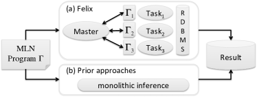
Figure 1: Felix breaks an input program, $\Gamma$, into several, smaller tasks (shown in Panel a), while prior approaches are monolithic (shown in Panel b).

Our goal is to use Markov Logic to construct a structured database of facts and then answer questions like “which Bulgarian leaders attended Sofia University and when?” with provenance from text. (Our system, Felix, answers Georgi Parvanov and points to a handful of sentences in a corpus to demonstrate its answer.) During the iterative process of constructing such a knowledge base from text and then using that knowledge base to answer sophisticated questions, we have found that it is critical to efficiently process structured queries over large volumes of structured data. And so, we have built Felix on top of an RDBMS. However, as we verify experimentally later in this paper, the scalability of previous RDBMS-based solutions to MLN inference [30] is still limited. Our key observation is that in many text processing applications, one must solve a handful of common subproblems, e.g., coreference resolution or classification. Some of these have been studied for decades, and so have specialized algorithms with higher scalability on these subproblems than the monolithic inference used by typical Markov Logic systems. Thus, our goal is to leverage the specialized algorithms for these subproblems to provide more scalable inference for general Markov Logic programs in an RDBMS. Figure 1 illustrates the difference at a high level between Felix and prior approaches: prior approaches, such as Alchemy [34] or Tuffy [30], are monolithic in that they attack the entire MLN inference problem with one algorithm; in constrast, Felix decomposes the problem into several small tasks.

To achieve this goal, we observe that the problem of inference in an MLN– and essentially any kind of statistical inference – can be cast as a mathematical optimization problem. Thus, we adapt techniques from the mathematical programming literature to MLN inference. In particular, we consider the idea of Lagrangian relaxation [6, p. 244] that allows one to decompose a complex optimization problem into multiple pieces that are hopefully easier to solve [51, 37]. Lagrangian relaxation is a widely deployed technique to cope with many difficult mathematical programming problems, and it is the theoretical underpinning of many state-of-the-art inference algorithms for graphical models, e.g., Belief Propagation [46]. In many – but not all – cases, a Lagrangian relaxation has the same optimal solution as the underlying original problem [6, 7, 51]. At a high level, Lagrangian relaxation gives us a message-passing protocol that resolves inconsistencies among conflicting predictions to accomplish joint-inference. Our system, Felix, does not actually construct the mathematical program, but uses Lagrangian relaxation as a formal guide to decompose an MLN program into multiple tasks and construct an appropriate message-passing scheme.

Our first technical contribution is an architecture to scalably perform MLN inference in an RDBMS using Lagrangian relaxation. Our architecture models each subproblem as a task that takes as input a set of relations, and outputs another set of relations. For example, our prototype of Felix implements specialized algorithms for classification and coreference resolution (coref); these tasks frequently occur in text-processing applications. By modeling tasks in this way, we are able to use SQL queries for all data movement in the system: both transforming the input data into an appropriate form for each task and encoding the message passing of Lagrangian relaxation between tasks. In turn, this allows Felix to leverage the mature, set-at-a-time processing power of an RBDMS to achieve scalability and efficiency. On all programs and datasets that we experimented with, our approach converges rapidly to the optimal solution of the Lagrangian relaxation. Our ultimate goal is to build high-quality applications, and we validate on several knowledge-base construction tasks that Felix achieves higher scalability and essentially identical result quality compared to prior MLN systems. More precisely, when prior MLN systems are able to scale, Felix converges to the same quality (and sometimes more efficiently). When prior MLN systems fail to scale, Felix can still produce high-quality results. We take this as evidence that Felix’s approach is a promising direction to scale up large-scale statistical inference. Furthermore, we validate that being able to integrate specialized algorithms is crucial for Felix’s scalability: after disabling specialized algorithms, Felix no longer scales to the same datasets.

Although the RDBMS provides some level of scalability for data movement inside Felix, the scale of data passed between tasks (via SQL queries) may be staggering. The reason is that statistical algorithms may produce huge numbers of combinations (say all pairs of potentially matching person mentions). The sheer sizes of intermediate results are often killers for scalability, e.g., the complete input to coreference resolution on an Enron dataset has $1.2\times 10^{11}$ tuples. The saving grace is that a task may access the intermediate data in an on-demand manner. For example, a popular coref algorithm repeatedly asks “given a fixed word $x$, tell me all words that are likely to be coreferent with $x$.” [3, 5]. Moreover, the algorithm only asks for a small fraction of such $x$. Thus, it would be wasteful to produce all possible matching pairs. Instead we can produce only those words that are needed on-demand (i.e., materialize them lazily). Felix considers a richer space of possible materialization strategies than simply eager or lazy: it can choose to eagerly materialize one or more subqueries responsible for data movement between tasks [33]. To make such decisions, Felix’s second contribution is a novel cost model that leverages the cost-estimation facility in the RDBMS coupled with the data-access patterns of the tasks. On the Enron dataset, our cost-based approach finds execution plans that achieve two orders of magnitude speedup over eager materialization and 2-3X speedup compared to lazy materialization.

Although Felix allows a user to provide any decomposition scheme, identifying decompositions could be difficult for some users, so we do not want to force users to specify a decomposition to use Felix. To support this, we need a compiler that performs task decomposition given a standard MLN program as input. Building on classical and new results in embedded dependency inference from the database theory literature [2, 1, 10, 14], we show that the underlying problem of compilation is $\Pi_{2}\mathbf{P}$-complete in easier cases, and undecidable in more difficult cases. To cope, we develop a sound (but not complete) compiler that takes as input an ordinary MLN program, identifies common tasks such as classification and coref, and then assigns those tasks to specialized algorithms.

To validate that our system can perform sophisticated knowledge-base construction tasks, we use the Felix system to implement a solution for the TAC-KBP (Knowledge Base Population) challenge. Given a 1.8M document corpus, the goal is to perform two related tasks: (1) entity linking: extract all entity mentions and map them to entries in Wikipedia, and (2) slot filling: determine relationships between entities. The reason for choosing this task is that it contains ground truth so that we can assess the results: We achieved F1=0.80 on entity linking (human performance is 0.90), and F1=0.34 on slot filling (state-of-the-art quality). In addition to KBP, we also use three information extraction (IE) datasets that have state-of-the-art solutions. On all four datasets, we show that Felix is significantly more scalable than monolithic systems such as Tuffy and Alchemy; this in turn enables Felix to efficiently process sophisticated MLNs and produce high-quality results. Furthermore, we validate that our individual technical contributions are crucial to the overall performance and quality of Felix.

$\mathtt{pSimHard}$(per1, per2) $\mathtt{pSimSoft}$(per1, per2) $\mathtt{oSimHard}$(org1, org2) $\mathtt{pSimSoft}$(org1, org2) $\mathtt{coOccurs}$(per, org) $\mathtt{homepage}$(per, page) $\mathtt{oMention}$(page, org) $\mathtt{faculty}$(org, per) $\mathtt{*affil}$(per, org) $\mathtt{*oCoref}$(org1, org2) $\mathtt{*pCoref}$(per1, per2)	$\mathtt{coOccurs}$(‘Ullman’, ‘Stanford Univ.’) $\mathtt{coOccurs}$(‘Jeff Ullman’, ‘Stanford’) $\mathtt{coOccurs}$(‘Gray’, ‘San Jose Lab’) $\mathtt{coOccurs}$(‘J. Gray’, ‘IBM San Jose’) $\mathtt{coOccurs}$(‘Mike’, ‘UC-Berkeley’) $\mathtt{coOccurs}$(‘Mike’, ‘UCB’) $\mathtt{coOccurs}$(‘Joe’, ‘UCB’) $\mathtt{faculty}$(‘MIT’, ‘Chomsky’) $\mathtt{homepage}$(‘Joe’, ‘Doc201’) $\mathtt{oMention}$(‘Doc201’, ‘IBM’) $\cdots$	weight rule $+\infty$ $\mathtt{pCoref}(p,p)$ ($F_{1}$) $+\infty$ $\mathtt{pCoref}(p1,p2)=>\mathtt{pCoref}(p2,p1)$ ($F_{2}$) $+\infty$ $\mathtt{pCoref}(x,y),\mathtt{pCoref}(y,z)=>\mathtt{pCoref}(x,z)$ ($F_{3}$) 6 $\mathtt{pSimHard}(p1,p2)=>\mathtt{pCoref}(p1,p2)$ ($F_{4}$) 2 $\mathtt{affil}(p1,o),\mathtt{affil}(p2,o),\mathtt{pSimSoft}(p1,p2)$ $=>\mathtt{pCoref}(p1,p2)$ ($F_{5}$) $+\infty$ $\mathtt{faculty}(o,p)=>\mathtt{affil}(p,o)$ ($F_{6}$) 8 $\mathtt{homepage}(p,d),\mathtt{oMention}(d,o)=>\mathtt{affil}(p,o)$ ($F_{7}$) 3 $\mathtt{coOccurs}(p,o1),\mathtt{oCoref}(o1,o2)=>\mathtt{affil}(p,o2)$ ($F_{8}$) 4 $\mathtt{coOccurs}(p1,o),\mathtt{pCoref}(p1,p2)=>\mathtt{affil}(p2,o)$ ($F_{9}$) $\ldots$
Schema	Evidence	Rules

Figure 2: An example MLN program that performs three tasks jointly: 1. discover affiliation relationships between people and organizations ($\mathtt{affil}$); 2. resolve coreference among people mentions ($\mathtt{pCoref}$); and 3. resolve coreference among organization mentions ($\mathtt{oCoref}$). The remaining eight relations are evidence relations. In particular, $\mathtt{coOccurs}$ stores person-organization co-occurrences; $*\mathtt{Sim}*$ relations are string similarities.

Outline

In Section 2, we describe related work. In Section 3, we describe a simple text application encoded as an MLN program, and the Lagrangian relaxation technique in mathematical programming. In Section 4, we present an overview of Felix’s architecture and some key concepts. In Section 5, we describe key technical challenges and how Felix addresses them: how to execute individual tasks with high performance and quality, how to improve the data movement efficiency between tasks, and how to automatically recognize specialized tasks in an MLN program. In Section 6, we use extensive experiments to validate the overall advantage of Felix as well as individual technical contributions.

2 Related Work

There is a trend to build semantically deep text applications with increasingly sophisticated statistical inference [52, 49, 43, 15]. We follow on this line of work. However, while the goal of prior work is to explore the effectiveness of different correlation structures on particular applications, our goal is to support general application development by scaling up existing statistical inference frameworks. Wang et al. [47] explore multiple inference algorithms for information extraction. However, their system focuses on managing low-level extractions in CRF models, whereas our goal is to use MLN to support knowledge base construction.

Felix specializes to MLNs. There are, however, other statistical inference frameworks such as PRMs [18], BLOG [28], Factorie [26, 50] , and PrDB [40]. Our hope is that the techniques developed here apply to these frameworks as well.

Researchers have proposed different approaches to improving MLN inference performance in the context of text applications. In StatSnowball [52], Zhu et al. demonstrate high quality results of an MLN-based approach. To address the scalability issue of generic MLN inference, they make additional independence assumptions in their programs. In contrast, the goal of Felix is to automatically scale up statistical inference while sticking to MLN semantics. Theobald et al. [44] design specialized MaxSAT algorithms that efficiently solve MLN programs of special forms. In contrast, we study how to scale general MLN programs. Riedel [35] proposed a cutting-plane meta-algorithm that iteratively performs grounding and inference, but the underlying grounding and inference procedures are still for generic MLNs. In Tuffy [30], the authors improve the scalability of MLN inference with an RDBMS, but their system is still a monolithic approach that consists of generic inference procedures.

As a classic technique, Lagrangian relaxation has been applied to closely related statistical models (i.e., graphical models) [20, 46]. However, there the input is directly a mathematical optimization problem and the granularity of decomposition is individual variables. In contrast, our input is a program in a high-level language, and we perform decomposition at the relation level inside an RDBMS.

Our materialization tradeoff strategy is related to view materialization and selection [41, 11] in the context of data warehousing. However, our problem setting is different: we focus on batch processing so that we do not consider maintenance cost. The idea of lazy-eager tradeoff in view materialization or query answering has also been applied to probabilistic databases [50]. However, their goal is efficiently maintaining intermediate results, rather than choosing a materialization strategy. Similar in spirit to our approach is Sprout [31], which considers lazy-versus-eager plans for when to apply confidence computation, but they do not consider inference decomposition.

3 Preliminaries

To illustrate how MLNs can be used in text-processing applications, we first walk through a program that extracts affiliations between people and organizations from Web text. We then describe how Lagrangian relaxation is used for mathematical optimization.

3.1 Markov Logic Networks in Felix

In text applications, a typical first step is to use standard NLP toolkits to generate raw data such as plausible mentions of people and organizations in a Web corpus and their co-occurrences. But transforming such raw signals into high-quality and semantically coherent knowledge bases is a challenging task. For example, a major challenge is that a single real-world entity may be referred to in many different ways, e.g., “UCB” and “UC-Berkeley”. To address such challenges, MLNs provide a framework where we can express logical assertions that are only likely to be true (and quantify such likelihood). Below we explain the key concepts in this framework by walking through an example.

Our system Felix is a middleware system: it takes as input a standard MLN program, performs statistical inference, and outputs its results into one or more relations that are stored in a relational database (PostgreSQL). An MLN program consists of three parts: schema, evidence, and rules. To tell Felix what data will be provided or generated, the user provides a schema. Some relations are standard database relations, and we call these relations evidence. Intuitively, evidence relations contain tuples that we assume are correct. In the schema of Figure 2, the first eight relations are evidence relations. For example, we know that ‘Ullman’ and ‘Stanford Univ.’ co-occur in some webpage, and that ‘Doc201’ is the homepage of ‘Joe’. In addition to evidence relations, there are also relations whose content we do not know, but we want the MLN program to predict; they are called query relations. In Figure 2, $\mathtt{affil}$ is a query relation since we want the MLN to predict affiliation relationships between persons and organizations. The other two query relations are $\mathtt{pCoref}$ and $\mathtt{oCoref}$, for person and organization coreference, respectively.

In addition to schema and evidence, we also provide a set of MLN rules that encode our knowledge about the correlations and constraints over the relations. An MLN rule is a first-order logic formula associated with an extended-real-valued number called a weight. Infinite-weighted rules are called hard rules, which means that they must hold in any prediction that the MLN system makes. In contrast, rules with finite weights are soft rules: a positive weight indicates confidence in the rule’s correctness. (In Felix, weights can be set by the user or automatically learned. We do not discuss learning in this work.)

• An important type of hard rule is a standard SQL query, e.g., to transform the results for use in the application. A more sophisticated example of hard rule is to encode that coreference has a transitive property, which is captured by the hard rule $F_{3}$. Rules $F_{8}$ and $F_{9}$ use person-organization co-occurrences ($\mathtt{coOccurs}$) together with coreference ($\mathtt{pCoref}$ and $\mathtt{oCoref}$) to deduce affiliation relationships ($\mathtt{affil}$). These rules are soft since co-occurrence in a webpage does not necessarily imply affiliation.

Intuitively, when a soft rule is violated, we pay a cost equal to the absolute value of its weight (described below). For example, if $\mathtt{coOccurs}$(‘Ullman’, ‘Stanford Univ.’) and $\mathtt{pCoref}$(‘Ullman’, ‘Jeff Ullman’), but not $\mathtt{affil}$(‘Jeff Ullman’, ‘Stanford Univ.’), then we pay a cost of 4 because of $F_{9}$. The goal of an MLN inference algorithm is to find a prediction that minimizes the sum of such costs.

Semantics

An MLN program defines a probability distribution over database instances (possible worlds). Formally, we first fix a schema $\sigma$ (as in Figure 2) and a domain $D$. Given as input a set of formulae $\bar{F}=F_{1},\dots,F_{N}$ with weights $w_{1},\dots,w_{N}$, they define a probability distribution over possible worlds (deterministic databases) as follows. Given a formula $F_{k}$ with free variables $\bar{x}=(x_{1},\cdots,x_{m})$, then for each $\bar{d}\in D^{m}$, we create a new formula $g_{\bar{d}}$ called a ground formula where $g_{\bar{d}}$ denotes the result of substituting each variable $x_{i}$ of $F_{k}$ with $d_{i}$. We assign the weight $w_{k}$ to $g_{\bar{d}}$. Denote by $G=(\bar{g},w)$ the set of all such weighted ground formulae of $\bar{F}$. We call the set of all tuples in $G$ the ground database. Let $w$ be a function that maps each ground formula to its assigned weight. Fix an MLN $\bar{F}$, then for any possible world (instance) $I$ we say a ground formula $g$ is violated if $w(g)>0$ and $g$ is false in $I$, or if $w(g)<0$ and $g$ is true in $I$. We denote the set of ground formulae violated in a world $I$ as $V(I)$. The cost of the world $I$ is

$$\mathrm{cost}_{\mathrm{mln}}(I)=\sum_{g\in V(I)}|w(g)|$$ (1)

Through $\mathrm{cost}_{\mathrm{mln}}$, an MLN defines a probability distribution over all instances using the exponential family of distributions (that are the basis for graphical models [46]):

$$\Pr[I]=Z^{-1}\exp\left\{-\mathrm{cost}_{\mathrm{mln}}(I)\right\}$$

where $Z$ is a normalizing constant.

Inference

There are two main types of inference with MLNs: MAP (maximum a posterior) inference, where we want to find a most likely world, i.e., a world with the lowest cost, and marginal inference, where we want to compute the marginal probability of each unknown tuple. Both types of inference are essentially mathematical optimization problems that are intractable, and so existing MLN systems implement generic (search/sampling) algorithms for inference. As a baseline, Felix implements generic algorithms for both types of inference as well. Although Felix supports both types of inference in our decomposition architecture, in this work we focus on MAP inference to simplify the presentation.

3.2 Lagrangian Relaxation

We illustrate the basic idea of Lagrangian relaxation with a simple example. Consider the problem of minimizing a real-valued function $f(x_{1},x_{2},x_{3})$. Lagrangian relaxation is a technique that allows us to divide and conquer a problem like this. For example, suppose that $f$ can be written as

$$f(x_{1},x_{2},x_{3})=f_{1}({x_{1}},{x_{2}})+f_{2}({x_{2}},{x_{3}}).$$

While we may be able to solve each of $f_{1}$ and $f_{2}$ efficiently, that ability does not directly lead to a solution to $f$ since $f_{1}$ and $f_{2}$ share the variable ${x_{2}}$. However, we can rewrite $\min_{x_{1},x_{2},x_{3}}f(x_{1},x_{2},x_{3})$ into the form

$$\min_{{x_{1},x_{21},x_{22},x_{3}}}f_{1}({x_{1}},{x_{21}})+f_{2}({x_{22}},{x_{3}})\text{ s.t. }{x_{21}}={x_{22}},$$

where we essentially made two copies of ${x_{2}}$ and enforce that they are identical. The significance of such rewriting is that we can apply Lagrangian relaxation to the equality constraint to decompose the formula into two independent pieces. To do this, we introduce a scalar variable $\lambda\in\mathds{R}$ (called a Lagrange multiplier) and define

$$g(\mathbf{\lambda})=\min_{x_{1},x_{21},x_{22},x_{3}}f_{1}({x_{1}},{x_{21}})+f_{2}({x_{22}},{x_{3}})+{\lambda}({x_{21}}-{x_{22}})$$

Then $\max_{\lambda}g(\lambda)$ is called the dual problem of the original minimization problem on $f$. Intuitively, The dual problem trades off a penalty for how much the copies $x_{21}$ and $x_{22}$ disagree with the original objective value. If the resulting solution of this dual problem is feasible for the original program (i.e., satisfies the equality constraint), then this solution is also an optimum of the original program [51, p. 168].

The key benefit of such relaxation is that, instead of a single problem on $f$, we can now compute $g(\lambda)$ by solving two independent problems (each problem is grouped by parentheses) that are hopefully (much) easier:

$$g(\lambda)=\left(\min_{x_{1},x_{21}}f_{1}(x_{1},x_{21})+\lambda x_{21}\right)+\left(\min_{x_{22},x_{3}}f_{2}(x_{22},x_{3})-\lambda x_{22}\right).$$

To compute $\max_{\lambda}g(\lambda)$, we can use standard techniques such as gradient descent [51, p. 174].

Notice that Lagrangian relaxation could be used for MLN inference: consider the case where $x_{i}$ are truth values of database tuples representing a possible world $I$ and define $f$ to be $\mathrm{cost}_{\mathrm{mln}}(I)$ as in Equation 1. (Felix can handle marginal inference with Lagrangian relaxation as well, but we focus on MAP inference to simplify presentation.)

Decomposition Choices

The Lagrangian relaxation technique leaves open the question of how to decompose a function $f$ in general and introduce equality constraints. These are the questions we need to answer first and foremost if we want to apply Lagrangian relaxation to MLNs. Furthermore, it is important that we can scale up the execution of the decomposed program on large datasets.

4 Architecture of Felix

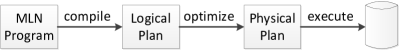
Figure 3: Execution Pipeline of Felix.

In this section, we provide an overview of the Felix architecture and some key concepts. We expand on further technical details in the next section. At a high level, the way Felix performs MLN inference resembles how an RDBMS performs SQL query evaluation: given an MLN program $\Gamma$, Felix transforms it in several phases as illustrated in Figure 3: Felix first compiles an MLN program into a logical plan of tasks. Then, Felix performs optimization (code selection) to select the best physical plan that consists of a sequence of statements that are then executed (by a process called the Master). In turn, the Master may call an RDBMS or statistical inference algorithms.

4.1 Compilation

In MLN inference, a variable of the underlying optimization problem corresponds to the truth value (for MAP inference) or marginal probability (for marginal inference) of a query relation tuple. While Lagrangian relaxation allows us to decompose an inference problem in arbitrary ways, Felix focuses on decompositions at the level of relations: Felix ensures that an entire relation is either shared between subproblems or exclusive to one subproblem. A key advantage of this is that Felix can benefit from the set-oriented processing power of an RDBMS. Even with this restriction, any partitioning of the rules in an MLN program $\Gamma$ is a valid decomposition. (For the moment, assume that all rules are soft; we come back to hard rules in Section 4.3.)

Formally, let $\Gamma=\{\phi_{i}\}$ be a set of MLN rules; denote by $\mathcal{R}$ the set of query relations and $\mathbf{x}_{R}$ the set of Boolean variables (i.e., unknown truth values) of $R\in\mathcal{R}$. Let $\Gamma_{1},\ldots,\Gamma_{k}$ be a decomposition of $\Gamma$, and $\mathcal{R}_{i}\subseteq\mathcal{R}$ the set of query relations referred to by $\Gamma_{i}$. Define $\mathbf{x}_{\mathcal{R}}=\cup_{R\in\mathcal{R}}\mathbf{x}_{R}$; similarly $\mathbf{x}_{\mathcal{R}_{i}}$. Then we can write the MLN cost function as

$$\min_{\mathbf{x}_{\mathcal{R}}}\mathrm{cost}_{\mathrm{mln}}^{\Gamma}(\mathbf{x}_{\mathcal{R}})=\min_{\mathbf{x}_{\mathcal{R}}}\sum_{i=1}^{k}\mathrm{cost}_{\mathrm{mln}}^{\Gamma_{i}}(\mathbf{x}_{\mathcal{R}_{i}})$$

To decouple the subprograms, we create a local copy of variables $\mathbf{x}^{i}_{\mathcal{R}_{i}}$ for each $\Gamma_{i}$, but also introduce Lagrangian multipliers $\mathbf{\lambda}_{R}^{j}\in\mathds{R}^{|\mathbf{x}_{R}|}$ for each $R\in\mathcal{R}$ and each $\Gamma_{j}$ s.t. $R\in\mathcal{R}_{j}$, resulting in the dual problem

$$\max_{\lambda}g(\lambda)$$

$$\equiv \max_{\lambda}\left\{\sum_{i=1}^{k}\min_{\mathbf{x}^{i}_{\mathcal{R}_{i}}}\left[\mathrm{cost}_{\mathrm{mln}}^{\Gamma_{i}}(\mathbf{x}^{i}_{\mathcal{R}_{i}})+\mathbf{\lambda}_{\mathcal{R}_{i}}^{i}\cdot\mathbf{x}^{i}_{\mathcal{R}_{i}}\right]\right\}$$

$$\textrm{subject to}\sum_{j:R\in\mathcal{R}_{j}}\mathbf{\lambda}_{R}^{j}=0\quad\forall R\in\mathcal{R}.$$

Thus, to perform Lagrangian relaxation on $\Gamma$, we need to augment the cost function of each subprogram with the $\mathbf{\lambda}_{\mathcal{R}_{i}}^{i}\cdot\mathbf{x}^{i}_{\mathcal{R}_{i}}$ terms. As illustrated in the example below, these additional terms are equivalent to adding singleton rules with the multipliers as weights. As a result, we can still solve the (augmented) subproblems $\Gamma^{\lambda}_{i}$ as MLN inference problems.

• Consider a simple Markov Logic program $\Gamma$:
  

  $1$	$\mathtt{GoodNews}(p)=>\mathtt{Happy}(p)$	$\phi_{1}$
  $1$	$\mathtt{BadNews}(p)=>\mathtt{Sad}(p)$	$\phi_{2}$
  $5$	$\mathtt{Happy}(p)<=>\neg\mathtt{Sad}(p)$	$\phi_{3}$

  
  

  where $\mathtt{GoodNews}$ and $\mathtt{BadNews}$ are evidence and the other two relations are queries. Consider the decomposition $\Gamma_{1}=\{\phi_{1}\}$ and $\Gamma_{2}=\{\phi_{2},\phi_{3}\}$. $\Gamma_{1}$ and $\Gamma_{2}$ share the relation $\mathtt{Happy}$; so we create two copies of this relation: $\mathtt{Happy_{1}}$ and $\mathtt{Happy_{2}}$, one for each subprogram. To relax the need that $\mathtt{Happy_{1}}$ and $\mathtt{Happy_{2}}$ be equal, we introduce Lagrange multipliers $\lambda_{p}$, one for each possible tuple $\mathtt{Happy}(p)$. We thereby obtain a new program $\Gamma^{\lambda}$:
  

$1$	$\mathtt{GoodNews}(p)=>\mathtt{Happy_{1}}(p)$	$\phi_{1}^{\prime}$
$\lambda_{p}$	$\mathtt{Happy_{1}}(p)$	$\varphi_{1}$
$1$	$\mathtt{BadNews}(p)=>\mathtt{Sad}(p)$	$\phi_{2}$
$5$	$\mathtt{Happy_{2}}(p)<=>\neg\mathtt{Sad}(p)$	$\phi_{3}^{\prime}$
$-\lambda_{p}$	$\mathtt{Happy_{2}}(p)$	$\varphi_{2}$

This program contains two subprograms, $\Gamma^{\lambda}_{1}=\{\phi_{1}^{\prime},\varphi_{1}\}$ and $\Gamma^{\lambda}_{2}=\{\phi_{2},\phi_{3}^{\prime},\varphi_{2}\}$, that can be solved independently.

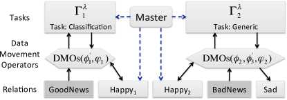
Figure 4: An example logical plan. Relations in shaded boxes are evidence relations. Solid arrows indicate data flow; dash arrows are control.

The output of compilation is a logical plan that consists of a bipartite graph between a set of subprograms (e.g., $\Gamma^{\lambda}_{i}$) and a set of relations (e.g., $\mathtt{GoodNews}$ and $\mathtt{Happy}$). There is an edge between a subprogram and a relation if the subprogram refers to the relation. In general, the decomposition could be either user-provided or automatically generated. In Sections 5.3 we discuss automatic decomposition.

4.2 Optimization

The optimization stage fleshes out the logical plan with code selection and generates a physical plan with detailed statements that are to be executed by a process in Felix called the Master. Each subprogram $\Gamma^{\lambda}_{i}$ in the logical plan is executed as a task that encapsulates a statistical algorithm that consumes and produces relations. The default algorithm assigned to each task is a generic MLN inference algorithm that can handle any MLN program [30]. However, as we will see in Section 5.1, there are several families of MLNs that have specialized algorithms with high efficiency and high quality. For tasks matching those families, we execute them with corresponding specialized algorithms.

The input/output relations of each task are not necessarily the relations in the logical plan. For example, the input to a classification task could be the results of some conjunctive queries translated from MLN rules. To model such indirection, we introduce data movement operators (DMOs), which are essentially datalog queries that map between MLN relations and task-specific relations. Roughly speaking, DMOs for specialized algorithms play a role that is similar to what grounding does for generic MLN inference. Given a task $\Gamma^{\lambda}_{i}$, it is the responsibility of the underlying algorithm to generate all necessary DMOs and register them with Felix. Figure 4 shows an enriched logical plan after code selection and DMO generation. DMOs are critical to the performance of Felix, and so we need to execute them efficiently. We observe that the overall performance of an evaluation strategy for a DMO depends on not only how well an RDBMS can execute SQL, but also how and how frequently a task queries this DMO – namely the access pattern of this task.

To expose the access patterns of a task to Felix, we model DMOs as adorned views [45]. In an adorned view, each variable in the head of a view definition is associated with a binding-type, which is either $\mathsf{b}$ (bound) or $\mathsf{f}$ (free). Given a DMO $Q$, denote by $\bar{x}^{\mathsf{b}}$ (resp. $\bar{x}^{\mathsf{f}}$) the set of bound (resp. free) variables in its head. Then we can view $Q$ as a function mapping an assignment to $\bar{x}^{\mathsf{b}}$ (i.e., a tuple) to a set of assignments to $\bar{x}^{\mathsf{f}}$ (i.e., a relation). Following the notation in Ullman [45], a query $Q$ of arity $a(Q)$ is written as $Q^{\alpha}(\bar{x})$ where $\alpha\in\left\{\mathsf{b},\mathsf{f}\right\}^{a(Q)}$. By default, all DMOs have the all-free binding pattern. But if a task exposes the access pattern of its DMOs, Felix can select evaluation strategies of the DMOs more informatively – Felix employs a cost-based optimizer for DMOs that takes advantage of both the RDBMS’s cost-estimation facility and the data-access pattern of a task (see Section 5.2).

• Say the subprogram $F_{1}$-$F_{5}$ in Figure 2 is executed as a task that performs coreference resolution on $\mathtt{pCoref}$, and Felix chooses the correlation clustering algorithm [3, 5] for this task. At this point, Felix knows the data-access properties of that algorithm (which essentially asks only for “neighboring” elements). Felix represents this using the following adorned view:

  $$\mathtt{DMO}^{\mathsf{bf}}(x,y) \leftarrow \mathtt{affil}(x,o),\mathtt{affil}(y,o),\mathtt{pSimSoft}(x,y).$$

  which is adorned as $\mathsf{bf}$. During execution, this coref task sends requests such as $x=\,$‘Joe’, and expects to receive a set of names $\{y\mid\mathtt{DMO}($‘Joe’$,y)\}$.

Sometimes Felix could deduce from the DMOs how a task may be parallelized (e.g., via key attributes), and takes advantage of such opportunities. The output of optimization is a DAG of statements. Statements are of two forms: (1) a prepared SQL statement; (2) a statement encoding the necessary information to run a task (e.g., the number of iterations an algorithm should run, data locations, etc.).

4.3 Execution

In Felix, a process called the Master coordinates the tasks by periodically updating the Lagrangian multiplier associated with each shared tuple (e.g., $\lambda_{p}$ in Example 4.1). Such an iterative updating scheme is called master-slave message passing. The goal is to optimize $\max_{\lambda}g(\lambda)$ using standard subgradient methods [51, p. 174]. Specifically, let $p$ be an unknown tuple of $R$, then at step $k$ the Master updates each $\lambda^{i}_{p}$ s.t. $R\in\mathcal{R}_{i}$ using the following rule:

$$\lambda^{i}_{p}=\lambda^{i}_{p}+\alpha_{k}\left(x^{i}_{p}-\frac{\sum_{j:R\in\mathcal{R}_{j}}x^{j}_{p}}{|\{j:R\in\mathcal{R}_{j}\}|}\right),$$

where $\alpha_{k}$ is the gradient step size for this update. A key novelty of Felix is that we can leverage the underlying RDBMS to efficiently compute the gradient on an entire relation. To see why, let $\lambda^{j}_{p}$ be the multipliers for a shared tuple $p$ of a relation $R$; $\lambda^{j}_{p}$ is stored as an extra attribute in each copy $j$ of $R$. Note that at each iteration, $\lambda^{j}_{p}$ changes only if the copies of $R$ do not agree on $p$ (e.g., exactly one copy has $p$ missing). Thus, we can update all $\lambda^{j}_{p}$’s with an outer join between the copies of $R$ using SQL. The gradient descent procedure stops either when all copies have reached an agreement (or only a very small portion disagrees) or when Felix has run a pre-specified maximum number of iterations.

Scheduling and Parallelism

Between two iterations of message passing, each task is executed until completion. If these tasks run sequentially (say due to limited RAM or CPU), then any order of execution would result in the same run time. On the other hand, if all tasks can run in parallel, then faster tasks would have to wait for the slowest task to finish until message passing could proceed. To better utilize CPU time, Felix updates the Lagrangian multipliers for a shared relation $R$ whenever all involved tasks have finished. Furthermore, a task is restarted when all shared relations of this task have been updated. If computation resources are abundant, Felix also considers parallelizing a task.

Initialization and Finalization

Let $\sigma=T_{1},\ldots,T_{n}$ be a sequence of all tasks obtained by a breadth-first traversal of the logical plan. At initial execution time, to bootstrap from the initial empty state, we sequentially execute the tasks in the order of $\sigma$, each task initializing its local copies of a relation by copying from the output of previous tasks. Then Felix performs the above master-slave message-passing scheme for several iterations; during this phase all tasks could run in parallel. At the end of execution, we perform a finalization step: we traverse $\sigma$ again and output the copy from $T^{R}_{\text{last}}$ for each query relation $R$, where $T^{R}_{\text{last}}$ is the last task in $\sigma$ that outputs $R$. To ensure that hard rules in the input MLN program are not violated in the final output, we insist that for any query relation $R$, $T^{R}_{\text{last}}$ respects all hard rules involving $R$. (We allow hard rules to be assigned to multiple tasks.) This guarantees that the output of the finalization step is a possible world for $\Gamma$ (provided that the hard rules are satisfiable).

5 Technical Details

Having set up the general framework, in this section, we discuss further technical challenges and solutions in Felix. First, as each individual task might be as complex as the original MLN, decomposition by itself does not automatically lead to high scalability. To address this issue, we identify several common statistical tasks with well-studied algorithms and characterize their correspondence with MLN subprograms (Section 5.1). Second, even when each individual task is able to run efficiently, sometimes the data movement cost may be prohibitive. To address this issue, we propose a novel cost-based materialization strategy for data movement operators (Section 5.2). Third, since the user may not be able to provide a good task decomposition scheme, it is important for Felix to be able to compile an MLN program into tasks automatically. To support this, we describe the compiler of Felix that automatically recognizes specialized tasks in an MLN program (Section 5.3).

5.1 Specialized Tasks

Task	Implementation
Simple Classification	Linear models [7]
Correlated Classification	Conditional Random Fields [24]
Coreference	Correlation clustering [3, 5]

Table 1: Example specialized tasks and their implementations in Felix.

By default, Felix solves a task (which is also an MLN program) with a generic MLN inference algorithm based on a reduction to MaxSAT [22], which is designed to solve sophisticated MLN programs. Ideally, when a task has certain properties indicating that it can be solved using a more efficient specialized algorithm, Felix should do so. Conceptually, the Felix framework supports all statistical tasks that can be modeled as mathematical programs. As an initial proof of concept, our prototype of Felix integrates two statistical tasks that are widely used in text applications: classification and coreference (see Table 1). These specialized tasks are well-studied and so have algorithms with high efficiency and high quality.

Classification Classification tasks are ubiquitous in text applications; e.g., classifying documents by topics or sentiments, and classifying noun phrases by entity types. In a classification task, we are given a set of objects and a set of labels; the goal is to assign a label to each object. Depending on the structure of the cost function, there are two types of classification tasks: simple classification and correlated classification.

In simple classification, given a model, the assignment of each object to a label is independent from other object labels. We describe a Boolean classification task for simplicity, i.e., our goal is to determine whether each object is in or out of a single class. The input to a Boolean classification task is a pair of relations: the model which can be viewed as a relation $M(\underline{f},w)$ that maps each feature $f$ to a single weight $w\in\mathds{R}$, and a relation of objects $I(o,f)$; if a tuple $(o,f)$ is in $I$ then object $o$ has feature $f$ (otherwise not). The output is a relation $R(o)$ that indicates which objects are members of the class ($R$ can also contain their marginal probabilities). For simple classification, the optimal $R$ can be populated by including those objects $o$ such that

$$\sum_{w:M(w,f)\text{ and }I(o,f)}w\geq 0$$

One can implement a simple classification task with SQL aggregates, which should be much more efficient than the MaxSAT algorithm used in generic MLN inference.

The twist in Felix is that the objects and the features of the model are defined by MLN rules. For example, the rules $F_{6}$ and $F_{7}$ in Figure 2 form a classification task that determines whether each $\mathtt{affil}$ tuple (considered as an object) holds. Said another way, each rule is a feature. So, Felix populates the model relation $M$ with two tuples: $M(F_{6},+\infty)$ and $M(F_{7},8)$, and populates the input relation $I$ by executing the conjunctive queries in $F_{6}$ and $F_{7}$; e.g., from $F_{7}$ Felix generates tuples of the form $I(P,O,F_{7})$, which indicates that the object $\mathtt{affil}(P,O)$ has the feature $F_{7}$. Operationally Felix performs such translation via DMOs that are also adorned with the task’s access patterns; e.g., the DMO for $I$ has the adornment $I^{\mathsf{bbf}}$ since Felix classifies each $\mathtt{affil}(P,O)$ independently.

Felix extends this basic model in two ways: (1) Felix implements multi-class classification by adding a class attribute to $M$ and $I$. (2) Felix also supports correlated classification: in addition to per-object features, Felix also allows features that span multiple objects. For example, in named entity recognition if we see the token “Mr.” the next token is very likely to be a person’s name. In general, one can form a graph where the nodes are objects and two objects are connected if there is a rule that refers to both objects. When this graph is acyclic, the task essentially consists of tree-structured CRF models that can be solved in polynomial time with dynamic programming algorithms [24].

Coreference Another common task is coreference resolution (coref), e.g., given a set of strings (say phrases in a document) we want to decide which strings represent the same real-world entity. These tasks are ubiquitous in text processing. The input to a coref task is a single relation $B(\underline{o1,o2},wgt)$ where $wgt=\beta_{o1,o2}\in\mathds{R}$ indicates how likely the objects $o1,o2$ are coreferent (with 0 being neutral). The output of a coref task is a relation $R(o1,o2)$ that indicates which pairs of objects are coreferent – $R$ is an equivalence relation, i.e., satisfying reflexivity, symmetry, and transitivity. Assuming that $\beta_{o1,o2}=0$ if $(o1,o2)$ is not in the key set of the relation $B$, then each valid $R$ incurs a cost (called disagreement cost)

$$\mathrm{cost}_{\mathrm{coref}}(R)=\sum_{\begin{subarray}{c}o1,o2:(o1,o2)\notin R\\ \mbox{ and }\beta_{o1,o2}>0\end{subarray}}|\beta_{o1,o2}|+\sum_{\begin{subarray}{c}o1,o2:(o1,o2)\in R\\ \mbox{ and }\beta_{o1,o2}<0\end{subarray}}|\beta_{o1,o2}|.$$

The goal of coref is to find a relation with the minimum cost:

$$R^{*}=\arg\min_{R}\mathrm{cost}_{\mathrm{coref}}(R).$$

Coreference resolution is a well-studied problem [16, 5]. The underlying inference problem is $\mathsf{NP}$-hard in almost all variants. As a result, there is a literature on approximation techniques (e.g., correlation clustering [3, 5]). Felix implements these algorithms for coreference tasks. In Figure 2, $F_{1}$ through $F_{5}$ consist of a coref task for the relation $\mathtt{pCoref}$. $F_{1}$ through $F_{3}$ encode the reflexivity, symmetry, and transitivity properties of $\mathtt{pCoref}$, and $\mathtt{F_{4}}$ and $\mathtt{F_{5}}$ essentially define the weights on the edges (similar to Arasu [5]) from which Felix constructs the relation $B$ (via DMOs).

5.2 Optimizing Data Movement Operators

Recall that data are passed between tasks and the RDBMS via data movement operators (DMOs). While the statistical algorithm inside a task may be very efficient (Section 5.1), DMO evaluation could be a major scalability bottleneck. An important goal of Felix’s optimization stage is to decide whether and how to materialize DMOs. For example, a baseline approach would be to materialize all DMOs. While this is a reasonable approach when a task repeatedly queries a DMO with the same parameters, in some cases, the result may be so large that an eager materialization strategy would exhaust available disk space. For example, on an Enron dataset, materializing the following DMO would require over 1TB of disk space:

$$\mathtt{DMO}^{\mathsf{bb}}(x,y) \leftarrow \mathtt{mention}(x,name1),\ \mathtt{mention}(y,name2),$$

$$\mathtt{mayref}(name1,z),\ \mathtt{mayref}(name2,z).$$

Moreover, some specialized tasks may inspect only a small fraction of their search space and so such eager materialization is inefficient. For example, one implementation of the coref task is a stochastic algorithm that examines data items roughly linear in the number of nodes (even though the input to coref contains a quadratic number of pairs of nodes) [5]. In such cases, it seems more reasonable to simply declare the DMO as a regular database view (or prepared statement) that is to be evaluated lazily during execution.

Felix is, however, not confined to fully eager or fully lazy. In Felix, we have found that intermediate points (e.g., materializing a subquery of a DMO $Q$) can have dramatic speed improvements (see Section 6.4). To choose among materialization strategies, Felix takes hints from the tasks: Felix allows a task to expose its access patterns, including both an adornment $Q^{\alpha}$ (see Section 4.2) and an estimated number of accesses $t$ on $Q$. (Operationally $t$ could be a Java function or SQL query to be evaluated against the base relations of $Q$.) Those parameters together with the cost-estimation facility of the underlying RDBMS (here, PostgreSQL) enable a System-R-style cost-based optimizer of Felix that explores all possible materialization strategies using the following cost model.

Felix Cost Model

To define our cost model, we introduce some notation. Let $Q^{\alpha}(\bar{x})\leftarrow g_{1},g_{2},\ldots,g_{k}$ be a DMO. Let $G=\{g_{i}|1\leq i\leq k\}$ be the set of subgoals of $Q$. Let $\mathcal{G}=\{G_{1},\ldots,G_{m}\}$ be a partition of $G$; i.e., $G_{j}\subseteq G$, $G_{i}\cap G_{j}=\emptyset$ for all $i\neq j$, and $\bigcup G_{j}=G$. Intuitively, a partition represents a possible materialization strategy: each element of the partition represents a query (or simply a relation) that Felix is considering materializing. That is, the case of one $G_{i}=G$ corresponds to a fully eager strategy. The case where all $G_{i}$ are singleton sets corresponds to a lazy strategy.

More precisely, define $Q_{j}(\bar{x}_{j})\leftarrow G_{j}$ where $\bar{x}_{j}$ is the set of variables in $G_{j}$ shared with ${\bar{x}}$ or any other $G_{i}$ for $i\neq j$. Then, we can implement the DMO with a regular database view $Q^{\prime}(\bar{x})\leftarrow Q_{1},\ldots,Q_{m}$. Let $t$ be the total number of accesses on $Q^{\prime}$ performed by the statistical task. We model the execution cost of a materialization strategy as:

$$\textrm{ExecCost}(Q^{\prime},t)=t\cdot\textrm{Inc}_{\alpha}(Q^{\prime})+\sum_{i=1}^{m}\textrm{Mat}(Q_{i})$$

$\textrm{Mat}(Q_{i})$ is the cost of eagerly materializing $Q_{i}$ and $\textrm{Inc}_{\alpha}(Q^{\prime})$ is the estimated cost of each query to $Q^{\prime}$ with adornment $\alpha$.

A significant implementation detail is that since the subgoals in $Q^{\prime}$ are not actually materialized, we cannot directly ask PostgreSQL for the incremental cost $\textrm{Inc}_{\alpha}(Q^{\prime})$. In our prototype version of Felix, we implement a simple approximation of PostgreSQL’s optimizer (that assumes incremental plans use only index-nested-loop joins), and so our results should be taken as a lower bound on the performance gains that are possible when materializing one or more subqueries. We provide more details on this approximation in Section C.3. Although the number of possible plans is exponential in the size of the largest rule in an input Markov Logic program, in our applications the individual rules are small. Thus, we can estimate the cost of each alternative, and we pick the one with the lowest $\mathrm{ExecCost}$.

5.3 Automatic Compilation

Properties	Symbol	Example
Reflexive	REF	$p(x,y)\implies p(x,x)$
Symmetric	SYM	$p(x,y)\implies p(y,x)$
Transitive	TRN	$p(x,y),p(y,z)\implies p(x,z)$
Key	KEY	$p(x,y),p(x,z)\implies y=z$
Not Recursive	NoREC	Can be defined w/o Recursion.
Tree Recursive	TrREC	See Equation 2

Table 2: Properties assigned to predicates by the Felix compiler. KEY refers to a non-trivial key. Recursive properties are derived from all rules; the other properties are derived from hard rules.

Task	Required Properties
Simple Classification	KEY, NoREC
Correlated Classification	KEY, TrREC
Coref	REF, SYM, TRN
Generic MLN Inference	none

Table 3: Tasks and their required properties.

So far we have assumed that the mappings between MLN rules, tasks, and algorithms are all specified by the user. However, ideally a compiler should be able to automatically recognize subprograms that could be processed as specialized tasks. In this section we describe a best-effort compiler that is able to automatically detect the presence of classification and coref tasks . To decompose an MLN program $\Gamma$ into tasks, Felix uses a two-step approach. Felix’s first step is to annotate each query predicate $p$ with a set of properties. An example property is whether or not $p$ is symmetric. Table 2 lists of the set of properties that Felix attempts to discover with their definitions; NoREC and TrREC are rule-specific. Once the properties are found, Felix uses Table 3 to list all possible options for a predicate. When there are multiple options, the current prototype of Felix simply chooses the first task to appear in the following order: (Coref, Simple Classification, Correlated Classification, Generic). This order intuitively favors more specific tasks. To compile an MLN into tasks, Felix greedily applies the above procedure to split a subset of rules into a task, and then iterates until all rules have been consumed. As shown below, property detection is non-trivial as the predicates are the output of SQL queries (or formally, datalog programs). Therefore, Felix implements a best-effort compiler using a set of syntactic patterns; this compiler is sound but not complete. It is interesting future work to design more sophisticated compilers for Felix.

Detecting Properties

The most technically difficult part of the compiler is determining the properties of the predicates (cf. [14]). There are two types of properties that Felix looks for: (1) schema-like properties of any possible worlds that satisfy $\Gamma$ and (2) graphical structures of correlations between tuples. For both types of properties, the challenge is that we must infer these properties from the underlying rules applied to an infinite number of databases. For example, SYM is the property:

“for any database $I$ that satisfies $\Gamma$, does the sentence $\forall x,y.\mathrm{pCoref}(x,y)\iff\mathrm{pCoref}(y,x)$ hold?”.

Since $I$ comes from an infinite set, it is not immediately clear that the property is even decidable. Indeed, REF and SYM are not decidable for Markov Logic programs.

Although the set of properties in Table 2 is motivated by considerations from statistical inference, the first four properties depend only on the hard rules in $\Gamma$, i.e., the constraints and (SQL-like) data transformations in the program. Let $\Gamma_{\infty}$ be the set of rules in $\Gamma$ that have infinite weight. We consider the case when $\Gamma_{\infty}$ is written as a datalog program.

Theorem 5.1.

Given a datalog program $\Gamma_{\infty}$, a predicate $p$, and a property $\theta$ deciding if for all input databases $p$ has property $\theta$ is undecidable if $\theta\in\left\{\text{REF},\text{SYM}\right\}$.

The above result is not surprising as datalog is a powerful language and containment is undecidable [2, ch. 12] (the proof reduces from containment). Moreover, the compiler is related to implication problems studied by Abiteboul and Hull (who also establish that generalizations of KEY and TRN problem are undecidable [1]). NoREC is the negation of the boundedness problem [10] which is undecidable.

In many cases, recursion is not used in $\Gamma_{\infty}$ (e.g., $\Gamma_{\infty}$ may consist of standard SQL queries that transform the data), and so a natural restriction is to consider $\Gamma_{\infty}$ without recursion, i.e., as a union of conjunctive queries.

Theorem 5.2.

Given a union of conjunctive queries $\Gamma_{\infty}$, deciding if for all input databases that satisfy $\Gamma_{\infty}$ the query predicate $p$ has property $\theta$ where $\theta\in\left\{\text{REF},\text{SYM}\right\}$ (Table 2) is decidable. Furthermore, the problem is $\Pi_{2}\mathsf{P}$-Complete. KEY and TRN are trivially false. NoRec is trivially true.

Still, Felix must annotate predicates with properties. To cope with the undecidability and intractability of finding out compiler annotations, Felix uses a set of sound (but not complete) rules that are described by simple patterns. For example, we can conclude that a predicate $R$ is transitive if program contains syntactically the rule $R(x,y),R(y,z)=>R(x,z)$ with weight $\infty$.

Ground Structure The second type of properties that Felix considers characterize the graphical structure of the ground database (in turn, this structure describes the correlations that must be accounted for in the inference process). We assume that $\Gamma$ is written as a datalog program (with stratified negation). The ground database is a function of both soft and hard rules in the input program, and so we consider both types of rules here. Felix’s compiler attempts to deduce a special case of recursion that is motivated by (tree-structured) conditional random fields that we call TrREC. Suppose that there is a single recursive rule that contains $p$ in the body and the head is of the form:

$$p(x,y),T(\underline{y},z)=>p(x,z)$$ (2)

where the first attribute of $T$ is a key and the transitive closure of $T$ is a partial order. In the ground database, $p$ will be “tree-structured”. MAP and marginal inference for such rules are in P-time [46, 40]. Felix has a regular expression to deduce this property.

6 Experiments

Although MLN inference has a wide range of applications, we focus on knowledge-base construction tasks. In particular, we use Felix to implement the TAC-KBP challenge; Felix is able to scale to the 1.8M-document corpus and produce results with state-of-the-art quality. In contrast, prior (monolithic) approaches to MLN inference crash even on a subset of KBP that is orders of magnitude smaller.

In Section 6.1, we compare the overall scalability and quality of Felix with prior MLN inference approaches on four datasets (including KBP). We show that, when prior MLN systems run, Felix is able to produce similar results but more efficiently; when prior MLN systems fail to scale, Felix can still generate high-quality results. In Sections 6.2, we demonstrate that the message-passing scheme in Felix can effectively reconcile conflicting predictions and has stable convergence behaviors. In Section 6.3, we show that specialized tasks and algorithms are critical for Felix’s high performance and scalability. In Section 6.4, we validate that the cost-based DMO optimization is crucial to Felix’s efficiency.

	#documents	#mentions
KBP	1.8M	110M
Enron	225K	2.5M
DBLife	22K	700K
NFL	1.1K	100K

Table 4: Statistics of input data. Note that MLN inference generates much larger intermediate data.

Datasets and Applications

Table 4 lists some statistics about the four datasets that we use for experiments: (1) KBP is a 1.8M-document corpus from TAC-KBP; the task is to perform two related tasks: a) entity linking: extract all entity mentions and map them to entries in Wikipedia, and b) slot filling: determine (tens of types of) relationships between entities. There is also a set of ground truths over a 2K-document subset (call it KBP-R) that we use for quality assessment. (2) NFL, where the task is to extract football game results (winners and losers) from sports news articles. (3) Enron, where the task is to identify person mentions and associated phone numbers in the Enron email dataset. There are two versions of Enron: Enron is the full dataset; Enron-R is a 680-email subset that we manually annotated person-phone ground truth on. We use Enron for performance evaluation, and Enron-R for quality assessment. (4) DBLife, where the task is to extract persons, organizations, and affiliation relationships between them from a collection of academic webpages. For DBLife, we use the ACM author profile data as ground truth.

MLN Programs

For KBP, we developed MLN programs that fuse a wide array of data sources including NLP results, Web search results, Wikipedia links, Freebase, etc. For performance experiments, we use our entity linking program (which is more sophisticated than slot filling). The MLN program on NFL has a conditional random field model as a component, with some additional common-sense rules (e.g., “a team cannot be both a winner and a loser on the same day.”) that are provided by another research project. To expand our set of MLN programs, we also create MLNs on Enron and DBLife by adapting rules in state-of-the-art rule-based IE approaches [25, 12]: Each rule-based program is essentially equivalent to an MLN-based program (without weights). We simply replace the ad-hoc reasoning in these deterministic rules by a simple statistical variant. For example, the DBLife program in Cimple [12] says that if a person and an organization co-occur with some regular expression context then they are affiliated, and ranks relationships by frequency of such co-occurrences. In the corresponding MLN we have several rules for several types of co-occurrences, and ranking is by marginal probabilities.

Experimental Setup

To compare with alternate implementations of MLNs, we consider two state-of-the-art MLN implementations: (1) Alchemy, the reference implementation for MLNs [13], and (2) Tuffy, an RDBMS-based implementation of MLNs [30]. Alchemy is implemented in C++. Tuffy and Felix are both implemented in Java and use PostgreSQL 9.0.4. Felix uses Tuffy as a task. Unless otherwise specified, all experiments are run on a RHEL5 workstation with two 2.67GHz Intel Xeon CPUs (24 total cores), 24 GB of RAM, and over 200GB of free disk space.

6.1 High-level Scalability and Quality

Scales?	Felix	Tuffy	Alchemy
KBP	Y	N	N
NFL	Y	Y	N
Enron	Y	N	N
DBLife	Y	N	N
KBP-R	Y	N	N
Enron-R	Y	Y	N

Table 5: Scalability of various MLN systems.

We empirically validate that Felix achieves higher scalability and essentially identical result quality compared to prior monolithic approaches. To support these claims, we compare the performance and quality of different MLN inference systems (Tuffy, Alchemy, and Felix) on the datasets listed above: KBP, Enron, DBLife, and NFL. In all cases, Felix runs its automatic compiler; parameters (e.g., gradient step sizes, generic inference parameters) are held constants across datasets. Tuffy and Alchemy have two sequential phases in their run time: grounding and search; results are produced only in the search phase. A system is deemed unscalable if it fails to produce any inference results within 6 hours. The overall scalability results are shown in Table 5.

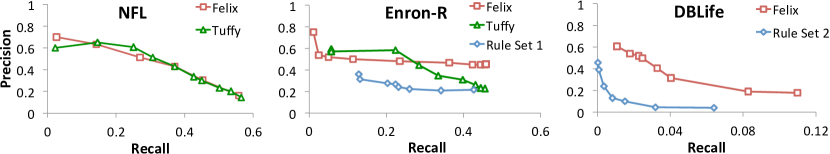
Figure 5: High-level quality results of various MLN systems. For each dataset, we plot a precision-recall curve of each system by varying $k$ in top-k results; missing curves indicate that a system does not scale on the corresponding dataset.

Quality Assessment

We perform quality assessment on four datasets: KBP-R, NFL, Enron-R, and DBLife. On each dataset, we run each MLN system for 4000 seconds with marginal inference. (After 4000 seconds, the quality of each system has stabilized.) For KBP-R, we convert the output to TAC’s query-answer format and compute the F1 score against the ground truth. For the other three datasets, we draw precision-recall curves: we take ranked lists of predictions from each system and measure precision/recall of the top-k results while varying the number of answers returned. The quality of each system is shown in Figure 5. System-dataset pairs that do not scale have no curves.

KBP & NFL

Recall that there are two tasks in KBP: entity linking and slot filling. On both tasks, Felix is able to scale to the 1.8M documents and after running about 5 hours on a 30-node parallel RDBMS, produce results with state-of-the-art quality[19]: We achieved an F1 score 0.80 on entity linking (human annotators’ performance is 0.90), and an F1 score 0.34 on slot filling (state-of-the-art quality). In contrast, Tuffy and Alchemy crashed even on the three orders of magnitude smaller KBP-R subset. Although also based on an RDBMS, Tuffy attempted to generate about $10^{11}$ and $10^{14}$ tuples on KBP-R and KBP, respectively.

To assess the quality of Felix as compared to monolithic inference, we also run the three MLN systems on NFL. Both Felix and Tuffy scale on the NFL data set, and as shown in Figure 5, produce results with similar quality. However, Felix is an order of magnitude faster: Tuffy took about an hour to start outputting results, whereas Felix’s quality converges after only five minutes. We validated that the reason is that Tuffy was not aware of the linear correlation structure of a classification task in the NFL program, and ran generic MLN inference in an inefficient manner.

Enron & DBLife

To expand our test cases, we consider two more datasets – Enron-R and DBLife – to evaluate the key question we try to answer: does Felix outperform monolithic systems in terms of scalability and efficiency? From Table 5, we see that Felix scales in cases where monolithic MLN systems do not. On Enron-R (which contains only 680 emails), we see that when both Felix and Tuffy scale, they achieve similar result quality. From Figure 5, we see that even when monolithic systems fail to scale (on DBLife), Felix is able to produce high-quality results.

To understand the result quality obtained by Felix, we also ran rule-based information-extraction programs for Enron-R and DBLife following practice described in the literature [27, 25, 12]. Recall that the MLN programs for Enron-R and DBLife were created by augmenting the deterministic rule sets with statistical reasoning. It should be noted that all systems can be improved with further tuning. In particular, the rules described in the literature (“Rule Set 1” for Enron-R [27, 25] and “Rule Set 2” for DBLife [12]) were not specifically optimized for high quality on the corresponding tasks. On the other hand, the corresponding MLN programs were generated in a constrained manner (as described in Section D.1). In particular, we did not leverage state-of-the-art NLP tools nor refine the MLN programs. With these caveats in mind, from Figure 5 we see that (1) on Enron-R, Felix achieves higher precision than Rule Set 1 given the same recall; and (2) on DBLife, Felix achieves higher recall than Rule Set 2 (i.e., Cimple [12]) at any precision level. This provides preliminary indication that statistical reasoning could help improve the result quality of knowledge-base construction tasks, and that scaling up MLN inference is a promising approach to high-quality knowledge-base construction. Nevertheless, it is interesting future work to more deeply investigate how statistical reasoning contributes to quality improvement over deterministic rules (e.g., Michelakis et al. [27]).

6.2 Effectiveness of Message Passing

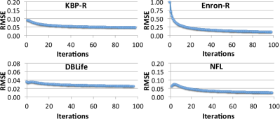
Figure 6: The RMSE between predictions from different tasks converges stably as Felix runs master-slave message passing.

We validate that the Lagrangian scheme in Felix can effectively reconcile conflicting predictions between related tasks to produce consistent output. Recall that Felix uses master-slave message passing to iteratively reconcile inconsistencies between different copies of a shared relation. To validate that this scheme is effective, we measure the difference between the marginal probabilities reported by different copies; we plot this difference as Felix runs 100 iterations. Specifically, we measure the root-mean-square-deviation (RMSE) between the marginal predictions of shared tuples between tasks. On each of the four datasets (i.e., KBP-R, Enron-R, DBLife, and NFL), we plot how the RMSE changes over time. As shown in Figure 9, Felix stably reduces the RMSE on all datasets to an eventual value of below $0.1$ – after about 80 iterations on Enron and after the very first iteration for the other three datasets. (As many statistical inference algorithms are stochastic, it is expected that the RMSE does not decrease to zero.) This demonstrates that Felix can effectively reconcile conflicting predictions, thereby achieving joint inference.

MLN inference is NP-hard, and so it is not always the case that Felix converges to the exact optimal solution of the original program. However, as we validated in the previous section, empirically Felix converges to close approximations of monolithic inference results (only more efficiently).

6.3 Importance of Specialized Tasks

We validate that the ability to integrate specialized tasks into MLN inference is key to Felix’s higher performance and scalability. To do this, we first show that specialized algorithms have higher efficiency than generic MLN inference on individual tasks. Second, we validate that specialized tasks are key to Felix’s scalability on MLN inference.

Task	System	Initial	Final	F1
Simple Classification	Felix	22 sec	22 sec	0.79
	Tuffy	113 sec	115 sec	0.79
	Alchemy	780 sec	782 sec	0.14
Correlated Classification	Felix	34 sec	34 sec	0.90
	Tuffy	150 sec	200 sec	0.09
	Alchemy	540 sec	560 sec	0.04
Coreference	Felix	3 sec	3 sec	0.60
	Tuffy	960 sec	1430 sec	0.24
	Alchemy	2870 sec	2890 sec	0.36

Table 6: Performance and quality comparison on individual tasks. “Initial” (resp. “Final”) is the time when a system produced the first (resp. converged) result. “F1” is the F1 score of the final output.

Quality & Efficiency

We first demonstrate that Felix’s specialized algorithms outperform generic MLN inference algorithms in both quality and performance when solving specialized tasks. To evaluate this claim, we run Felix, Tuffy, and Alchemy on three MLN programs that each encode one of the following tasks: simple classification, correlated classification, and coreference. We use a subset of the Cora dataset for coref, and a subset of the CoNLL 2000 chunking dataset for classification. The results are shown in Table 6. While it always takes less than a minute for Felix to finish each task, Tuffy and Alchemy take much longer. Moreover, the quality of Felix is higher than Tuffy and Alchemy. As expected, Felix can achieve exact optimal solutions for classification, and nearly optimal approximation for coref, whereas Tuffy and Alchemy rely on a general-purpose SAT counting algorithm. Nevertheless, the above micro benchmark results are typically drowned out in larger-scale applications, where the quality difference tend to be smaller compared to the results here.

Scalability

To demonstrate that specialized tasks are crucial to the scalability of Felix, we remove specialized tasks from Felix and re-evaluate whether Felix is still able to scale to the four datasets (KBP, Enron, DBLife, and NFL). The results are as follows: after disabling classification, Felix crashes on KBP and DBLife; after disabling coref, Felix crashes on Enron. On NFL, although Felix is still able to run without specialized tasks, its performance slows down by an order of magnitude (from less than five minutes to more than one hour). These results suggest that specialized tasks are critical to Felix’s high scalability and performance.

6.4 Importance of DMO Optimization

We validate that Felix’s cost-based approach to data movement optimization is crucial to the efficiency of Felix. To do this, we run Felix on subsets of Enron with various sizes in three different settings: 1) Eager, where all DMOs are evaluated eagerly; 2) Lazy, where all DMOs are evaluated lazily; 3) Opt, where Felix decides the materialization strategy for each DMO based on the cost model in Section 5.2.

	E-5k	E-20k	E-50k	E-100k
Eager	83 sec	15 min	134 min	641 min
Lazy	42 sec	5 min	22 min	78 min
Opt	29 sec	2 min	7 min	25 min

Table 7: DMO efficiency under different settings.

We observed that overall Opt is substantially more efficient than both Lazy and Eager, and found that the deciding factor is the efficiency of the DMOs of the coref tasks. Thus, we specifically measure the total run time of individual coref tasks, and compare the results in Table 7. Here, E-$x$k for $x\in\left\{5,20,50,100\right\}$ refers to a randomly selected subset of $x$k emails in the Enron corpus. We observe that the performance of the eager materialization strategy degrades rapidly as the dataset size increases. The lazy strategy performs much better. The cost-based approach can further achieve 2-3X speedup. This demonstrates that our cost-based materialization strategy for data movement operators is crucial to the efficiency of Felix.

7 Conclusion and Future Work

We present our Felix approach to MLN inference that uses relation-level Lagrangian relaxation to decompose an MLN program into multiple tasks and solve them jointly. Such task decomposition enables Felix to integrate specialized algorithms for common tasks (such as classification and coreference) with both high efficiency and high quality. To ensure that tasks can communicate and access data efficiently, Felix uses a cost-based materialization strategy for data movement. To free the user from manual task decomposition, the compiler of Felix performs static analysis to find specialized tasks automatically. Using these techniques, we demonstrate that Felix is able to scale to complex knowledge-base construction applications and produce high-quality results whereas previous MLN systems have much poorer scalability . Our future work is in two directions: First, we plan to apply our key techniques (in-database Lagrangian relaxation and cost-based materialization) to other inference problems. Second, we plan to extend Felix with new logical tasks and physical implementations to support broader applications.

Appendix A Notations

Table 8 defines some common notation that is used in the following sections.

Notation	Definition
$a,b,\ldots,\alpha,\beta,\ldots$	Singular (random) variables
$\boldsymbol{a}$, $\boldsymbol{b}$,$\ldots$, $\boldsymbol{\alpha}$, $\boldsymbol{\beta}$,$\ldots$	Vectorial (random) variables
$\boldsymbol{\mu}^{\prime}\cdot\boldsymbol{\nu}$	Dot product between vectors
$|\boldsymbol{\mu}|$	Length of a vector or size of a set
$\boldsymbol{\mu}_{i}$	$i^{th}$ element of a vector
$\hat{\alpha},\hat{\boldsymbol{\alpha}}$	A value of a variable

Table 8: Notations

Appendix B Theoretical Background of the Operator-based Approach

In this section, we discuss the theoretical underpinning of Felix’s operator-based approach to MLN inference. Recall that Felix first decomposes an input MLN program based on a predefined set of operators, instantiates those operators with code selection, and then executes the operators using ideas from dual decomposition. We first justify our choice of specialized subtasks (i.e., Classification, Sequential Labeling, and Coref) in terms of two compilation soundness and language expressivity properties:

1. Given an MLN program, the subprograms obtained by Felix’s compiler indeed encode specialized subtasks such as classification, sequential labeling, and coref.

2. MLN as a language is expressive enough to encode all possible models in the exponential family of each subtask type; specifically, MLN subsumes logistic regression (for classification), conditional random fields (for labeling), and correlation clustering (for coref).

We then describe how dual decomposition is used to coordinate the operators in Felix for both MAP and marginal inference while maintaining the semantics of MLNs.

B.1 Consistent Semantics

B.1.1 MLN Program Solved as Subtasks

In this section, we show that the decomposition of an MLN program produced by Felix’s compiler indeed corresponds to the subtasks defined in Section 4.2.

Simple Classification

Suppose a classification operator (i.e., task) for a query relation $R(k,v)$ consists of key-constraint hard rules together with rules $r_{1},...,r_{t}$ (with weights $w_{1},...,w_{t}$) . As per Felix’s compilation procedure, the following holds: 1) $R(k,v)$ has a key constraint (say $k$ is the key); and 2) none of the selected rules are recursive with respect to $R$.

Let $k_{0}$ be a fixed value of $k$. Since $k$ is a possible-world key for $R(k,v)$, we can partition the set of all possible worlds into sets based on their $v$ for $R(k_{0},v)$ (and whether there is any value $v$ make $R(k,v)$ true). Let $\mathcal{W}_{v_{i}}=\{W\mid W\models R(k_{0},v_{i})\}$ and $\mathcal{W}_{\perp}$ where $R(k_{0},v)$ is false for all $v$. Define $Z(\mathcal{W})=\sum_{w\in\mathcal{W}}\exp\{-cost(w)\}$. Then according to the semantics of MLN,

$$\Pr[R(k,v_{0})]=\frac{Z(\mathcal{W}_{v_{0}})}{Z(\mathcal{W}_{\perp})+\sum_{v\in\mathbb{D}}Z(\mathcal{W}_{v})}$$

It is immediate from this that each class is disjoint. It is also clear that, conditioned on the values of the rule bodies, each of the $R$ are independent.

Correlated Classification

Suppose a correlated classification operator outputs a relation $R(k,v)$ and consists of hard-constraint rules together with ground rules $r_{1},...r_{t}$ (with weights $w_{1},...,w_{t}$). As per Felix’s compilation procedure, the following holds:

• $R(k,v)$ has a key constraint (say $k$ is the key);

• The rules $r_{i}$ satisfy the TrREC property.

Consider the following graph: the nodes are all possible values for the key $k$ and there is an edge $(k,k^{\prime})$ if $k$ appears in the body of $k^{\prime}$. Every node in this graph has outdegree at most $1$. Now suppose there is a cycle: But this contradicts the definition of a strict partial order. In turn, this means that this graph is a forest. Then, we identify this graph with a graphical model structure where each node is a random variable with domain $\mathbb{D}$. This is a tree-structured Markov random field. This justifies the rules used by Felix’s compiler for identifying labeling operators. Again, conditioned on the rule bodies any grounding is a tree-shaped graphical model.

Coreference Resolution

A coreference resolution subtask involving variables $y_{1},...y_{n}$ infers about an equivalent relation $R(y_{i},y_{j})$. The only requirement of this subtask is that the result relation $R(.,.)$ be reflexive, symmetric and transitive. Felix ensures these properties by detecting corresponding hard rules directly.

B.1.2 Subtasks Represented as MLN programs

We start by showing that all probabilistic distributions in the discrete exponential family can be represented by an equivalent MLN program. Therefore, if we model the three subtasks using models in the exponential family, we can express them as an MLN program. Fortunately, for each of these subtasks, there are popular exponential family models: 1) Logistic Regression (LR) for Classification, 2) Conditional Random Filed (CRF) for Labeling and 3) Correlation Clustering for Coref.

Definition B.1 (Exponential Family).

We follow the definition in [46]. Given a vector of binary random variables $\boldsymbol{x}\in\mathcal{X}$, let $\boldsymbol{\phi}:\mathcal{X}\rightarrow\{0,1\}^{d}$ be a binary vector-valued function. For a given $\boldsymbol{\phi}$, let $\boldsymbol{\theta}\in\mathbb{R}^{d}$ be a vector of real number parameters. The exponential family distribution over $\boldsymbol{x}$ associated with $\boldsymbol{\phi}$ and $\boldsymbol{\theta}$ is of the form:

$$\Pr_{\boldsymbol{\theta}}[\boldsymbol{x}]=\exp\{-\boldsymbol{\theta}\cdot\boldsymbol{\phi}(\boldsymbol{x})-A(\boldsymbol{\theta})\},$$

where $A(\boldsymbol{\theta})$ is known as log partition function: $A(\boldsymbol{\theta})=\log\sum_{\boldsymbol{x}\in\mathcal{X}}\exp\{-\boldsymbol{\theta}\cdot\boldsymbol{\phi}(\boldsymbol{x})\}$.

This definition extends to multinomial random variables in a straightforward manner. For simplicity, we only consider binary random variables in this section.

• Consider a textbook logistic regressor over a random variable $x\in\{0,1\}$:

  $$\Pr[x=1]=\frac{1}{1+\exp\{\sum_{i}-\beta_{i}f_{i}\}},$$

  where $f_{i}\in\{0,1\}$’s are known as features of $x$ and $\beta_{i}$’s are regression coefficients of $f_{i}$’s. This distribution is actually in the exponential family: Let $\boldsymbol{\phi}$ be a binary vector-valued function whose $i^{th}$ entry equals to $\boldsymbol{\phi}_{i}(x)=(1-x)f_{i}$. Let $\boldsymbol{\theta}$ be a vector of real numbers whose $i^{th}$ entry $\boldsymbol{\theta}_{i}=\beta_{i}$. One can check that

  $$\Pr[x=1]= \frac{\exp\left\{-\boldsymbol{\theta}\cdot\boldsymbol{\phi}(1)\right\}}{\exp\left\{-\boldsymbol{\theta}\cdot\boldsymbol{\phi}(1)\right\}+\exp\left\{-\boldsymbol{\theta}\cdot\boldsymbol{\phi}(0)\right\}}$$

  $$= \frac{1}{1+\exp\left\{\sum_{i}-\beta_{i}f_{i}\right\}}$$

The exponential family has a strong connection with the maximum entropy principle and graphic models. For all the three tasks we are considering, i.e., classification, labeling and coreference, there are popular exponential family models for each of them.

Proposition B.1.

Given an exponential family distribution over $\boldsymbol{x}\in\mathcal{X}$ associated with $\boldsymbol{\phi}$ and $\boldsymbol{\theta}$, there exists an MLN program $\Gamma$ that defines the same probability distribution as $\Pr_{\boldsymbol{\theta}}[\boldsymbol{x}]$. The length of the formula in $\Gamma$ is at most linear in $|\boldsymbol{x}|$, and the number of formulas in $\Gamma$ is at most exponential in $|\boldsymbol{x}|$.

Proof.

Our proof is by construction. Each entry of $\boldsymbol{\phi}$ is a binary function $\phi_{i}(\boldsymbol{x})$, which partitions $\mathcal{X}$ into two subsets: $\mathcal{X}_{i}^{+}=\{\boldsymbol{x}|\phi_{i}(\boldsymbol{x})=1\}$ and $\mathcal{X}_{i}^{-}=\{\boldsymbol{x}|\phi_{i}(\boldsymbol{x})=0\}$. If $\theta_{i}\geq 0$, for each $\hat{\boldsymbol{x}}\in\mathcal{X}_{i}^{+}$, introduce a rule:

$$\theta_{i}~{}~{}~{}\bigvee_{1\leq j\leq|\boldsymbol{x}|}R(x_{j},1-\hat{x_{j}}).$$

If $\theta_{i}<0$, for each $\hat{\boldsymbol{x}}\in\mathcal{X}_{i}^{+}$, insert a rule:

$$-\theta_{i}~{}~{}~{}\bigwedge_{1\leq j\leq|\boldsymbol{x}|}R(x_{j},\hat{x_{j}}).$$

We add these rules for each $\phi_{i}(.)$, and also add the following hard rule for each variable $x_{i}$:

$$\infty~{}~{}~{}R(x_{i},0)\quad<=>\quad\neg R(x_{i},1).$$

It is not difficult to see $\Pr[\forall x_{i},R(x_{i},\hat{x_{i}})=1]=\Pr_{\boldsymbol{\theta}}[\hat{\boldsymbol{x}}]$. In this construction, each formula has length $|\boldsymbol{x}|$ and there are $\sum_{i}(|\mathcal{X}_{i}|+1)$ formulas in total, which is exponential in $|\boldsymbol{x}|$ in the worst case. ∎

Similar constructions apply to the case where $\boldsymbol{x}$ is a vector of multinomial random variables.

We then show that Logistic Regression, Conditional Random Field and Correlation Clustering all define probability distributions in the discrete exponential family, and the number of formulas in their equivalent MLN program $\Gamma$ is polynomial in the number of random variables.

Logistic Regression

In Logistic Regression, we model the probability distribution of Bernoulli variable $y$ conditioned on $x_{1},...,x_{k}\in\{0,1\}$ by

$$\Pr[y=1]=\frac{1}{1+\exp\{-(\beta_{0}+\sum_{i}\beta_{i}x_{i})\}}$$

Define $\phi_{i}(y)=(1-y)x_{i}$ ($\phi_{0}(y)=1-y$) and $\theta_{i}=\beta_{i}$, we can see $\Pr[y=1]$ is in the exponential family defined as in Definition B.1. For each $\phi_{i}(y)$, there is only one $y$ that can get positive value from $\phi_{i}$, so there are at most $k+1$ formulas in the equivalent MLN program.

Conditional Random Field

In Conditional Random Field, we model the probability distribution using a graph $G=(V,E)$ where $V$ represents the set of random variables $\boldsymbol{y}=\{y_{v}:v\in V\}$. Conditioned on a set of random variables $\boldsymbol{x}$, CRF defines the distribution:

$$\Pr[\boldsymbol{y}|\boldsymbol{x}]\propto{} \exp\{\sum_{v\in V,k}\lambda_{k}f_{k}(v,y_{v},\boldsymbol{x})$$

$$+\sum_{(v_{1},v_{2})\in E,l}\mu_{l}g_{l}((v_{1},v_{2}),y_{v_{1}},y_{v_{2}},\boldsymbol{x})\}$$

This is already in the form of exponential family. Because each function $f_{k}(v,-,\boldsymbol{x})$ or $g_{l}((v_{1},v_{2}),-,-,\boldsymbol{x})$ only relies on 1 or 2 random variables, the resulting MLN program has at most $O(|E|+|V|)$ formulas. In the current prototype of Felix, we only consider linear chain CRFs, where $|E|=O(|V|)$.

Correlation Clustering

Correlation clustering is a form of clustering for which there are efficient algorithms that have been shown to scale to instances of the coref problem with millions of mentions. Formally, correlation clustering treats the coref problem as a graph partitioning problem. The input is a weighted undirected graph $G=(V,f)$ where $V$ is the set of mentions with weight function $f:V^{2}\rightarrow\mathbb{R}$. The goal is to find a partition $\mathcal{C}=\{C_{i}\}$ of $V$ that minimizes the disagreement cost:

$$cost_{cc}(\mathcal{C})=\sum_{\begin{subarray}{c}(v1,v2)\in V^{2}\\ v_{1}\neq v_{2}\\ \exists C_{i},v_{1}\in C_{i}\wedge v_{2}\in C_{i}\\ f(u,v)<0\end{subarray}}|f(v_{1},v_{2})|+\sum_{\begin{subarray}{c}(v1,v2)\in V^{2}\\ v_{1}\neq v_{2}\\ \exists C_{i},v_{1}\in C_{i}\wedge v_{2}\not\in C_{i}\\ f(u,v)>0\end{subarray}}|f(v_{1},v_{2})|$$

We can define the probability distribution over $\mathcal{C}$ similarly as MLN:

$$\Pr[\mathcal{C}]\propto\exp\{-cost_{cc}(\mathcal{C})\}$$

Specifically, let the binary predicate $coref(v_{1},v_{2})$ indicate whether $v_{1}\neq v_{2}\in V$ belong to the same cluster. First introduce three hard rules enforcing the reflexivity, symmetry, and transitivity properties of $coref$. Next, for each $v_{1}\neq v_{2}\in V$, introduce a singleton rule $coref(v_{1},v_{2})$ with weight $f(v_{1},v_{2})$. It’s not hard to show that the above distribution holds for this MLN program.

B.2 Dual Decomposition for MAP and Marginal Inference

In this section, we formally describe the dual decomposition framework used in Felix to coordinate the operators. We start by formalizing MLN inference as an optimization problem. Then we show how to apply dual decomposition on these optimization problems.

B.2.1 Problem Formulation

Suppose an MLN program $\Gamma$ consists of a set of ground MLN rules $\mathcal{R}=\{r_{1},...,r_{m}\}$ with weights ($w_{1},...,w_{m}$). Let ${X}=\{x_{1},...,x_{n}\}$ be the set of boolean random variables corresponding to the ground atoms occurring in $\Gamma$. Each MLN rule $r_{i}$ introduces a function $\phi_{i}$ over the set of random variables $\pi_{i}\subseteq{X}$ mentioned in $r_{i}$: $\phi_{i}(\pi_{i})=1$ if $r_{i}$ is violated and $0$ otherwise. Let $\boldsymbol{w}$ be a vector of weights. Define vector $\boldsymbol{\phi}({X})=(\phi_{1}(\pi_{1}),...,\phi_{m}(\pi_{m}))$. Given a possible world $\boldsymbol{x}\in 2^{X}$, the cost can be represented:

$$cost(\boldsymbol{x})=\boldsymbol{w}\cdot\boldsymbol{\phi}(\boldsymbol{x})$$

Suppose Felix decides to solve $\Gamma$ with $t$ operators $O_{1},...,O_{t}$. Each operator $O_{i}$ contains a set of rules $\mathcal{R}_{i}\subseteq\mathcal{R}$. The set $\{\mathcal{R}_{i}\}$ forms a partition of $\mathcal{R}$. Let the set of random variables for each operator be ${X}_{i}=\cup_{r_{j}\in\mathcal{R}_{i}}\pi_{j}$. Let $n_{i}=|{X}_{i}|$. Thus, each operator $O_{i}$ essentially solves the MLN program defined by random variables ${X}_{i}$ and rules $\mathcal{R}_{i}$. Given $\boldsymbol{w}$, define $\boldsymbol{w}^{i}$ to be the weight vector whose entries equal $\boldsymbol{w}$ if the corresponding rule appears in $\mathcal{R}_{i}$ and 0 otherwise. Because $\mathcal{R}_{i}$ forms a partition of $\mathcal{R}$, we know $\sum_{i}\boldsymbol{w}^{i}=\boldsymbol{w}$. For each operator $O_{i}$, define an $n$-dim vector $\boldsymbol{\mu}_{i}({X})$, whose $j^{th}$ entry equals $x_{j}$ if $x_{j}\in{X}_{i}$ and 0 otherwise. Define $n$-dim vector $\boldsymbol{\mu}({X})$ whose $j^{th}$ entry equals $x_{j}$. Similarly, let $\boldsymbol{\phi}({X}_{i})$ be the projection of $\boldsymbol{\phi}({X})$ onto the rules in operator $O_{i}$.

• We use the two sets of rules for classification and labeling in Section 5.1 as a running example. For a simple sentence Packers win. in a fixed document $D$ which contains two phrases $P_{1}=$ “Packers” and $P_{2}=$ “win”, we will get the following set of ground formulae :

  $\infty$	$\mathtt{label}(D,p,l1),\mathtt{label}(D,p,l2)=>l1=l2$	$(r_{l1})$
  10	$\mathtt{next}(D,P_{1},P_{2}),\mathtt{token}(P_{2},\text{`wins'})=>\mathtt{label}(D,P_{1},W)$	$(r_{l2})$
  1	$\mathtt{label}(D,P_{1},W),\mathtt{next}(D,P_{1},P_{2})=>!\mathtt{label}(D,P_{2},W)$	$(r_{l3})$
  10	$\mathtt{label}(D,P_{1},W),\mathtt{referTo}(P_{1},GreenBay)=>\mathtt{winner}(GreenBay)$	$(r_{c1})$
  10	$\mathtt{label}(D,P_{1},L),\mathtt{referTo}(P_{1},GreenBay)=>\mathtt{!winner}(GreenBay)$	$(r_{c2})$

After compilation, Felix would assign $r_{l1}$, $r_{l2}$ and $r_{l3}$ to a labeling operator $O_{L}$, and $r_{c1}$ and $r_{c2}$ to a classification operator $O_{C}$. For each of $\{\mathtt{winner}(GreenBay)$, $\mathtt{label}(D,P_{1},W)$, $\mathtt{label}(D,P_{1},L)$, $\mathtt{label}(D,P_{2},W)$, $\mathtt{label}(D,P_{2},L)\}$ we have a binary random variable associated with it. Each rule introduces a function $\phi$, for example, the function $\phi_{l2}$ introduced by $r_{l2}$ is:

$$\phi_{l2}(\mathtt{label}(D,P_{1},W))=\begin{cases}1&\text{if $\mathtt{label}(D,P_{1},W)=\textrm{False}$}\\ 0&\text{if $\mathtt{label}(D,P_{1},W)=\textrm{True}$}\end{cases}$$

The labeling operator $O_{L}$ essentially solves the MLN program with variables ${X}_{L}=\{\mathtt{label}(D,P_{1},W)$, $\mathtt{label}(D,P_{1},L)$, $\mathtt{label}(D,P_{2},W)$, $\mathtt{label}(D,P_{2},L)\}$ and rules $\mathcal{R}_{L}=\{r_{l1}$, $r_{l2}$, $r_{l3}\}$. Similarly $O_{C}$ solves the MLN program with variables ${X}_{C}=\{\mathtt{winner}(GreenBay)$, $\mathtt{label}(D,P_{1},W)$ $\mathtt{label}(D,P_{1},L)\}$ and rules $\mathcal{R}_{C}=\{r_{c1}$, $r_{c2}\}$. Note that these two operators share the variables $\mathtt{label}(D,P_{1},W)$ and $\mathtt{label}(D,P_{1},L)$.

B.2.2 MAP Inference

MAP inference in MLNs is to find an assignment ${\boldsymbol{x}}$ to $X$ that minimizes the cost:

$$\min_{{\boldsymbol{x}}\in\{0,1\}^{n}}\boldsymbol{w}\cdot\boldsymbol{\phi}({\boldsymbol{x}}).$$ (3)

Each operator $O_{i}$ performs MAP inference on ${X}_{i}$:

$$\min_{{\boldsymbol{x}}_{i}\in\{0,1\}^{n_{i}}}\boldsymbol{w}^{i}\cdot\boldsymbol{\phi}({\boldsymbol{x}}_{i}).$$ (4)

Our goal is to reduce the problem represented by Eqn. 3 into subproblems represented by Eqn. 4. Eqn. 3 can be rewritten as

$$\min_{\boldsymbol{x}\in\{0,1\}^{n}}\sum_{1\leq i\leq t}\boldsymbol{w}^{i}\cdot\boldsymbol{\phi}(\boldsymbol{x}_{i}).$$

Clearly, the difficulty lies in that, for $i\neq j$, ${X}_{i}$ and ${X}_{j}$ may overlap. Therefore, we introduce a copy of variables for each $O_{i}$: ${X}_{i}^{C}$. Eqn. 3 now becomes:

$$\min_{{\boldsymbol{x}}_{i}^{C}\in\{0,1\}^{n_{i}},{\boldsymbol{x}}} ~{}~{}\sum_{i}\boldsymbol{w}^{i}\cdot\boldsymbol{\phi}(\boldsymbol{x}_{i}^{C})$$ (5)

$$s.t. ~{}~{}\forall i\quad\boldsymbol{x}_{i}^{C}=\boldsymbol{x}.$$

The Lagrangian of this problem is:

$$\mathcal{L}(\boldsymbol{x},\boldsymbol{x}_{1}^{C},...,\boldsymbol{x}_{t}^{C},\boldsymbol{\nu}_{1},...,.\boldsymbol{\nu}_{t})$$ (6)

$$= \sum_{i}\boldsymbol{w}^{i}\cdot\boldsymbol{\phi}(\boldsymbol{x}_{i}^{C})+\boldsymbol{\nu}_{i}\cdot(\boldsymbol{\mu}_{i}(\boldsymbol{x}_{i}^{C})-\boldsymbol{\mu}_{i}(\boldsymbol{x}))$$

Thus, we can relax Eqn. 3 into

$$\max_{\boldsymbol{\nu}}\left\{\sum_{i}\left[\min_{\boldsymbol{x}_{i}\in\{0,1\}^{n_{i}}}\boldsymbol{w}^{i}\cdot\boldsymbol{\phi}(\boldsymbol{x}_{i}^{C})+\boldsymbol{\nu}_{i}\cdot\boldsymbol{\mu}_{i}(\boldsymbol{x}_{i}^{C})\right]-\max_{\boldsymbol{x}}\sum_{i}\boldsymbol{\nu}_{i}\cdot\boldsymbol{\mu}_{i}(\boldsymbol{x})\right\}$$

The term $\max_{\boldsymbol{x}}\sum_{i}\boldsymbol{\nu}_{i}\cdot\boldsymbol{\mu}_{i}(\boldsymbol{x})=\infty$ unless for each variable $x_{j}$,

$$\sum_{O_{i}:x_{j}\in{X}_{i}}\boldsymbol{\nu}_{i,j}=0.$$

Converting this into constraints, we get

$$\max_{\boldsymbol{\nu}} ~{}~{}\left\{\sum_{i}\min_{\boldsymbol{x}_{i}\in\{0,1\}^{n_{i}}}\boldsymbol{w}^{i}\cdot\boldsymbol{\phi}(\boldsymbol{x}_{i}^{C})+\boldsymbol{\nu}_{i}\cdot\boldsymbol{\mu}_{i}(\boldsymbol{x}_{i}^{C})\right\}$$

$$s.t. ~{}~{}\forall x_{j}\quad\sum_{O_{i}:x_{j}\in{X}_{i}}\boldsymbol{\nu}_{i,j}=0$$

We can apply sub-gradient methods on $\boldsymbol{\nu}$. The dual decomposition procedure in Felix works as follows:

1. Initialize $\boldsymbol{\nu}_{1}^{(0)},...,\boldsymbol{\nu}_{t}^{(0)}$.

2. At step $k$ (starting from 0):

   1. For each operator $O_{i}$, solve the MLN program consisting of: 1) original rules in this operator, which are characterized by $\boldsymbol{w}^{i}$; 2) additional priors on each variables in ${X}_{i}$, which are characterized by $\boldsymbol{\nu}_{i}^{(k)}$.

   2. Get the MAP inference results $\hat{\boldsymbol{x}_{i}^{C}}$.

3. Update $\boldsymbol{\nu}_{i}$:
   $\boldsymbol{\nu}_{i,j}^{(k+1)}=\boldsymbol{\nu}_{i,j}^{(k)}-\lambda\left(\hat{\boldsymbol{x}_{i,j}^{C}}-\frac{\sum_{l:x_{j}\in X_{l}}\hat{\boldsymbol{x}_{l,j}^{C}}}{|\{l:x_{j}\in X_{l}\}|}\right)$

• Consider the MAP inference on program in Example B.2.1. As $O_{L}$ and $O_{C}$ share two random variables: $x_{w}=\mathtt{label}(D,P_{1},W)$ and $x_{l}=\mathtt{label}(D,P_{1},L)$, we have a copy of them for each operator: $x_{w,O_{L}}^{C}$, $x_{l,O_{L}}^{C}$ for $O_{L}$; and $x_{w,O_{C}}^{C}$, $x_{l,O_{C}}^{C}$ for $O_{C}$. Therefore, we have four $\nu$: $\nu_{w,O_{L}}$, $\nu_{l,O_{L}}$ for $O_{L}$; and $\nu_{w,O_{C}}$, $\nu_{l,O_{C}}$ for $O_{C}$. Assume we initialize each $\nu_{-}^{(0)}$ to $0$ at the first step.

  We start by performing MAP inference on $O_{L}$ and $O_{C}$ respectively. In this case, $O_{L}$ will get the result:

  $$x_{w,O_{L}}^{C}=1$$

  $$x_{l,O_{L}}^{C}=0$$

  $O_{C}$ admits multiple possible worlds minimizing the cost; for example, it may outputs

  $$x_{w,O_{C}}^{C}=0$$

  $$x_{l,O_{C}}^{C}=0$$

  which has cost 0. Assume the step size $\lambda=0.5$. We can update $\nu$ to:

  $$\nu_{w,O_{L}}^{(1)}= -0.25$$

  $$\nu_{w,O_{C}}^{(1)}= 0.25$$

  $$\nu_{l,O_{L}}^{(1)}= 0$$

  $$\nu_{l,O_{C}}^{(1)}= 0$$

  Therefore, when we use these $\nu_{-}^{(1)}$ to conduct MAP inference on $O_{L}$ and $O_{C}$, we are equivalently adding

  -0.25 $\mathtt{label}(D,P_{1},W)$

  $(r_{l}^{\prime})$

into $O_{L}$ and

0.25 $\mathtt{label}(D,P_{1},W)$

$(r_{c}^{\prime})$

into $O_{C}$. Intuitively, one may interpret this procedure as the information that “$O_{L}$ prefers $\mathtt{label}(D,P_{1},W)$ to be true” being passed to $O_{C}$ via $r_{c}^{\prime}$.

B.2.3 Marginal Inference

The marginal inference of MLNs aims at computing the marginal distribution (i.e., the expectation since we are dealing with boolean random variables):

$$\hat{\boldsymbol{\mu}}=\mathbb{E}_{\boldsymbol{w}}[\boldsymbol{\mu}({X})].$$ (7)

The sub-problem of each operator is of the form:

$$\hat{\boldsymbol{\mu}}_{O}=\mathbb{E}_{\boldsymbol{w}_{O}}[\boldsymbol{\mu}_{O}({X}_{O})].$$ (8)

Again, the goal is to use solutions for Eqn. 8 to solve Eqn. 7.

We first introduce some auxiliary variables. Recall that $\boldsymbol{\mu}({X})$ corresponds to the set of random variables, and $\boldsymbol{\phi}({X})$ corresponds to all functions represented by the rules. We create a new vector $\boldsymbol{\xi}$ by concatenating $\boldsymbol{\mu}$ and $\boldsymbol{\phi}$: $\boldsymbol{\xi}({X})=(\boldsymbol{\mu}^{T}({X}),\boldsymbol{\phi}^{T}({X}))$. We create a new weight vector $\boldsymbol{\theta}=(0,...,0,\boldsymbol{w}^{T})$ which is of the same length as $\boldsymbol{\xi}$. It is not difficult to see that the marginal inference problem equivalently becomes:

$$\hat{\boldsymbol{\xi}}=\mathbb{E}_{\boldsymbol{\theta}}[\boldsymbol{\xi}({X})].$$ (9)

Similarly, we define $\boldsymbol{\theta}_{O}$ for operator $O$ as $\boldsymbol{\theta}_{O}=(0,...,0,\boldsymbol{w}^{T}_{O})$. We also define a set of $\boldsymbol{\theta}$: $\Theta_{O}$, which contains all vectors with entries corresponding to random variables or cliques not appear in operator $O$ as zero. The partition function $A(\boldsymbol{\theta})$ is:

$$A(\boldsymbol{\theta})=\sum_{\mathcal{X}}\exp\{-\boldsymbol{\theta}\cdot\boldsymbol{\xi}(\mathcal{X})\}$$

The conjugate dual to $A$ is:

$$A^{*}(\boldsymbol{\xi})=\sup_{\boldsymbol{\theta}}\{\boldsymbol{\theta}\cdot\boldsymbol{\xi}-A(\boldsymbol{\theta})\}$$

A classic result of variational inference [46] shows that

$$\hat{\boldsymbol{\xi}}=\arg\sup_{\boldsymbol{\xi}\in\mathcal{M}}\{\boldsymbol{\theta}\cdot\boldsymbol{\xi}-A^{*}(\boldsymbol{\xi})\},$$ (10)

where $\mathcal{M}$ is the marginal polytope. Recall that $\hat{\boldsymbol{\xi}}$ is our goal (see Eqn. 9). Similar to MAP inference, we want to decompose Eqn. 10 into different operators by introducing copies of shared variables. We first try to decompose $A^{*}(\boldsymbol{\xi})$. In $A^{*}(\boldsymbol{\xi})$, we search $\boldsymbol{\theta}$ on all possible values for $\boldsymbol{\theta}$. If we only search on a subset of $\boldsymbol{\theta}$, we can get a lower bound:

$$A^{*O}(\boldsymbol{\xi})=\sup_{\boldsymbol{\theta}\in\Theta_{O}}\{\boldsymbol{\theta}\cdot\boldsymbol{\xi}-A^{*}(\boldsymbol{\xi})\}\leq A^{*}(\boldsymbol{\xi}).$$

Therefore,

$$-A^{*}(\boldsymbol{\xi})\leq\frac{1}{m}\sum_{O}-A^{*O}(\boldsymbol{\xi}),$$

where $m$ is the number of operators. We approximate $\hat{\boldsymbol{\xi}}$ using this bound:

$$\hat{\boldsymbol{\xi}}=\arg\sup_{\boldsymbol{\xi}\in\mathcal{M}}\{\boldsymbol{\theta}\cdot\boldsymbol{\xi}-\frac{1}{m}\sum_{O}A^{*O}(\boldsymbol{\xi})\},$$

which is an upper bound of the original goal. We introduce copies of $\boldsymbol{\xi}$:

$$\hat{\boldsymbol{\xi}}=\arg\sup_{\boldsymbol{\xi}^{O_{i}}\in\mathcal{M},\boldsymbol{\xi}} ~{}~{}\{\sum_{O}\boldsymbol{\theta}_{O}\cdot\boldsymbol{\xi}^{O}-\frac{1}{m}\sum_{O}A^{*O}(\boldsymbol{\xi}^{O})\}$$

$$s.t. ~{}~{}\boldsymbol{\xi}^{O}_{e}=\boldsymbol{\xi}_{e},\forall e\in\mathcal{X}_{O}\cup\mathcal{R}_{O},\forall O$$

The Lagrangian of this problem is:

$$\mathcal{L}(\boldsymbol{\xi},\boldsymbol{\xi}^{O_{1}},...,\boldsymbol{\xi}^{O_{t}},\boldsymbol{\nu}_{1},...,\boldsymbol{\nu}_{t}) =\sum_{O}\left\{\boldsymbol{\theta}_{O}\cdot\boldsymbol{\xi}^{O}-\frac{1}{m}A^{*O}(\boldsymbol{\xi}^{O})\right\}$$

$$~{}~{}+\sum_{i}\boldsymbol{\nu}_{i}\cdot(\boldsymbol{\xi}^{O_{i}}-\boldsymbol{\xi}),$$

where $\boldsymbol{\nu}_{i}\in\Theta_{i}$, which means only the entries corresponding to random variables or cliques that appear in operator $O_{i}$ are allowed to have non-zero values. We get the relaxation:

$$\min_{\boldsymbol{\nu}_{i}\in\Theta_{i}}\sum_{i}\sup_{\boldsymbol{\xi}^{O_{i}}\in\mathcal{M}}\left\{\boldsymbol{\theta}_{i}\cdot\boldsymbol{\xi}^{O_{i}}-\frac{1}{m}A^{*O_{i}}(\boldsymbol{\xi}^{O_{i}})+\boldsymbol{\nu}_{i}\cdot\boldsymbol{\xi}^{O_{i}}\right\}$$

$$-\min_{\boldsymbol{\xi}}\sum_{i}\boldsymbol{\nu}_{i}\cdot\boldsymbol{\xi}$$

Considering the $\min_{\boldsymbol{\xi}}\sum_{i}\boldsymbol{\nu}_{i}\cdot\boldsymbol{\xi}$ part. This part is equivalent to a set of constraints:

$$\sum_{O_{i}:x\in{X}_{i}}\boldsymbol{\nu}_{i,x}= 0,\forall x\in{X}$$

$$\boldsymbol{\nu}_{i,x}= 0,\forall x\not\in{X}$$

Therefore, we are solving:

$$\min_{\boldsymbol{\nu}_{i}\in\Theta_{i}} ~{}~{}\sum_{i}\sup_{\boldsymbol{\xi}^{O_{i}}\in\mathcal{M}}\left\{m\boldsymbol{\theta}_{i}\cdot\boldsymbol{\xi}^{O_{i}}-A^{*O_{i}}(\boldsymbol{\xi}^{O_{i}})+\boldsymbol{\nu}_{i}\cdot\boldsymbol{\xi}^{O_{i}}\right\}$$

$$s.t., ~{}~{}\sum_{O_{i}:x\in{X}_{i}}\boldsymbol{\nu}_{i,x}=0,\forall x\in{X}$$

$$~{}~{}\boldsymbol{\nu}_{i,x}=0,\forall x\not\in{X}$$

Note the factor $m$ in front of $\boldsymbol{\theta}_{i}$; it implies that we multiply the weights in each subprogram by $m$ as well. Then we can apply sub-gradient method on $\boldsymbol{\nu}_{i}$:

1. Initialize $\boldsymbol{\nu}_{1}^{(0)},...,\boldsymbol{\nu}_{t}^{(0)}$.

2. At step $k$ (start from 0):

   1. For each operator $O_{i}$, solve the MLN program consists of: 1) original rules in this operator, which is characterized by $m\boldsymbol{\theta}_{i}$; 2) additional priors on each variables in $\mathcal{X}_{i}$, which is characterized by $\boldsymbol{\nu}_{i}^{(k)}$.

   2. Get the marginal inference results $\hat{\boldsymbol{\xi}_{i}^{C}}$.

3. Update $\boldsymbol{\nu}_{i}^{(k+1)}$:
   $\boldsymbol{\nu}_{i,j}^{(k+1)}=\boldsymbol{\nu}_{i,j}^{(k)}-\lambda\left(\hat{\boldsymbol{\xi}_{i,j}^{C}}-\frac{\sum_{l:x_{j}\in{X}_{l}}\hat{\boldsymbol{\xi}_{l,j}^{C}}}{|\{l:x_{j}\in{X}_{l}\}|}\right)$

• Consider the marginal inference on the case in Example B.2.1. Similar to the example for MAP inference, we have copies of random variables: $\xi_{w,O_{L}}^{C}$, $\xi_{l,O_{L}}^{C}$ for $O_{L}$; and $\xi_{w,O_{C}}^{C}$, $\xi_{l,O_{C}}^{C}$ for $O_{C}$. We also have four $\nu$: $\nu_{w,O_{L}}$, $\nu_{l,O_{L}}$ for $O_{L}$; and $\nu_{w,O_{C}}$, $\nu_{l,O_{C}}$ for $O_{C}$. Assume we initialize each $\nu_{-}^{(0)}$ to $0$ at the first step.

  We start by conducting marginal inference on $O_{L}$ and $O_{C}$ respectively. In this case, $O_{L}$ will get the result:

  $$\xi_{w,O_{L}}^{C}=0.99$$

  $$\xi_{l,O_{L}}^{C}=0.01$$

  while $O_{C}$ will get:

  $$\xi_{w,O_{C}}^{C}=0.5$$

  $$\xi_{l,O_{C}}^{C}=0.5$$

  Assume the step size $\lambda=0.5$. We can update $\nu$ as:

  $$\nu_{w,O_{L}}^{(1)}= -0.12$$

  $$\nu_{w,O_{C}}^{(1)}= 0.12$$

  $$\nu_{l,O_{L}}^{(1)}= 0.12$$

  $$\nu_{l,O_{C}}^{(1)}= -0.12$$

  Therefore, when we use these $\nu_{-}^{(1)}$ to conduct marginal inference on $O_{L}$ and $O_{C}$, we are equivalantly adding

  -0.12	$\mathtt{label}(D,P_{1},W)$	$(r_{l1}^{\prime})$
  0.12	$\mathtt{label}(D,P_{1},L)$	$(r_{l2}^{\prime})$

into $O_{L}$ and

0.12	$\mathtt{label}(D,P_{1},W)$	$(r_{c1}^{\prime})$
-0.12	$\mathtt{label}(D,P_{1},L)$	$(r_{c2}^{\prime})$

into $O_{C}$. Intuitively, one may interpret this procedure as the information that “$O_{L}$ prefers $\mathtt{label}(D,P_{1},W)$ to be true” being passed to $O_{C}$ via $r_{c}^{\prime}$.

Appendix C Additional Details of System Implementation

In this section, we provide additional details of the Felix system. The first part of this section focuses on the compiler. We prove some complexity results of property-annotation used in the compiler and describe how to apply static analysis techniques originally used in the Datalog literature for data partitioning. Then we describe the physical implementation for each logical operator in the current prototype of Felix. We also describe the cost model used for the materialization trade-off.

C.1 Compiler

C.1.1 Complexity Results

In this section, we first prove the decidability of the problem of annotating properties for arbitrary Datalog programs. Then we prove the $\Pi_{2}\mathsf{P}$-completeness of the problem of annotating $\{REF,SYM\}$ given a Datalog program without recursion.

Recursive Programs

If there is a single rule with query relation $Q$ of the form $Q(x,y)<=Q1(x),Q2(y)$, then that $\left\{\text{REF},\text{SYM}\right\}$ of $Q$ is decidable if and only if $Q1$ or $Q2$ is empty or $Q1\equiv Q2$. We assume that $Q1$ and $Q2$ are satisfiable. If there is an instance where $Q1(a)$ is true and $Q2$ is false for all values. Then there is another world (with all fresh constants) where $Q2$ is true (and does not return $a$). Thus, to check REF and SYM for $Q$, we need to decide equivalence of datalog queries. Equivalence of datalog queries is undecidable [2, ch. 12]. Since containment and boundedness for monadic datalog queries is decidable, a small technical wrinkle is that while $Q1$ and $Q2$ are of arity one (monadic) their bodies may contain other recursive (higher arity) predicates.

Complexity for Nonrecursive Program

The above section assumes that we are given an arbitrary Datalog program $\Gamma$. In this section, we show that the problem of annotating REF and SYM given a nonrecursive Datalog program is $\Pi_{2}\mathsf{P}$-complete. We allow inequalities in the program.

We first prove the hardness. Similar to the above section, we need to decide $Q1\equiv Q2$. The difference is that $Q1$ and $Q2$ do not have recursions. Since our language allows us to express conjunctive queries with inequality constraints, this established $\Pi_{2}\mathsf{P}$ hardness [23].

We now prove the membership in $\Pi_{2}\mathsf{P}$. We first translate the problem of property-annotation to the containment problem of Datalog programs, which has been studied for decades [9, 23] and the complexity is in $\Pi_{2}\mathsf{P}$ for Datalog programs without recursions but with inequalities. We will show that, even though the rules for checking symmetric property is recursive, it can be represented by a set of non-recursive rules, therefore the classic results still hold.

We thus limit ourselves to non-recursive MLN programs. Given an MLN program $\Gamma$ which is the union of conjunctive queries and a relation $Q$ to which we will annotate properties, all hard rules related to $Q$ can be represented as:

$$Q():- G_{1}() P_{1}$$ ()

$$Q():- G_{2}()$$

$$...$$

$$Q():- G_{n}()$$

where each $G_{i}()$ contains a set of subgoals. To annotate whether a property holds for the relation $Q()$, we test whether some rules hold for all database instances $I$ generated by the above program $P_{1}$. For example, for the symmetric property, we label $Q()$ as symmetric if and only if $Q(x,y)=>Q(y,x)$ holds. We call this rule the testing rule. Suppose the testing rule is $Q():-T()$, we create a new program:

$$Q():- G_{1}() P_{2}$$ ()

$$Q():- G_{2}()$$

$$...$$

$$Q():- G_{n}()$$

$$Q():- T()$$

Given a database $D$, let $P_{1}(D)$ be the result of applying program $P_{1}$ to $D$ (using Datalog semantics). The testing rule holds for all $P_{1}(D)$ if and only if $\forall D$, $P_{2}(D)\subseteq P_{1}(D)$. In other words, $P_{2}$ is contained by $P_{1}$ ($P_{2}\subseteq P_{1}$). For reflexive property, whose testing rule is $Q(x,x):-\mathcal{D}(x)$ (where $\mathcal{D}()$ is the domain of $x$), both $P_{1}$ and $P_{2}$ are non-recursive and the checking of containment is in $\Pi_{2}\mathsf{P}$ [23].

We then consider the symmetric property, whose testing rule is recursive. This is difficult at first glance because the containment of recursive Datalog program is undecidable. However, for this special case, we can show it is much easier. For the sake of simplicity, we consider a simplified version of $P_{1}$ and $P_{2}$:

$$Q(x,y):-G(x,y,z) P_{1}^{\prime}$$ ()

$$Q(x,y):- G(x,y,z) P_{2}^{\prime}$$ ()

$$Q(x,y):- Q(y,x)$$

We construct the following program:

$$Q(x,y):- G(x,y,z) P_{3}$$ ()

$$Q(x,y):- G(y,x,z)$$

It is easy to show $P_{2}^{\prime}=P_{3}$, therefore, we can equivalently check whether $P_{3}\subseteq P_{1}^{\prime}$, which is in $\Pi_{2}\mathsf{P}$ since neither of the programs is recursive.

C.1.2 Patterns Used by the Compiler

Felix exploits a set of regular expressions for property annotation. This set of regular expressions forms a best-effort compiler, which is sound but not complete. Table 9 shows these patterns. In Felix, a pattern consists of two components – a template and a boolean expression. A template is a constraint on the “shape” of the formula. For example, one template for SYM looks like $P_{1}(a,b)\vee!P_{2}(c,d)$, which means we only consider rules whose disjunction form contains exactly two binary predicates with opposite senses. Rules that pass the template-matching are considered further using the boolean expression. If one rule passes the template-matching step, we can have a set of assignments for each predicate $P$ and variable $a,b,...$. The boolean expression is a first order logic formula on the assignment. For example, the boolean expression for the above template is $(a=d)\wedge(b=c)\wedge(P_{1}=P_{2})$, which means the assignment of $P_{1}$ and $P_{2}$ must be the same, and the assignment of variables $a,b,c,d$ must satisfy $(a=d)\wedge(b=c)$. If there is an assignment that satisfies the boolean expression, we say this Datalog rule matches with this pattern and will be annotated with corresponding labels.

Property	Pattern
	Template	Condition
REF	$P_{1}(a,b)$	$a=b$
	$P_{1}(a,b)\vee!R_{1}(c)\vee!R_{2}(d)$	$a=c,b=d,R_{1}=R_{2},P_{1}\neq R_{i}$
SYM	$P_{1}(a,b)\vee!P_{2}(c,d)$	$a=d,b=c,P_{1}=P_{2}$
	$P_{1}(a,b)\vee!R_{1}(c)\vee!R_{2}(d)$	$a=c,b=d,R_{1}=R_{2},P_{1}\neq R_{i}$
TRN	$!P_{1}(a,b)\vee!P_{2}(c,d)\vee$$P_{3}(e,f)$	$b=c$, $a=e$, $d=f$, $P_{1}=P_{2}=P_{3}$
KEY	$!P_{1}(a,b)\vee!P_{2}(e,f)\vee[c=d]$	$a=e$, $b=c$, $d=f$,$P_{1}=P_{2}$
NoREC	$R_{1}()\vee\ldots\vee R_{n}()\vee P_{1}()$	$P_{1}\neq R_{i}$
	$R_{1}()\vee\ldots\vee R_{n}()\vee!P_{1}()$	$P_{1}\neq R_{i}$
TrRec	$P_{1}(a,b)\vee T(c,d)\vee P_{2}(e,f)$	$b=c$, $d=f$, $a=e$, $P_{1}=P_{2}$, $T(c,d)=[d=c+x],x\neq 0$
	$P_{1}(a,b)\vee T(c,d)\vee P_{2}(e,f)$	$b=c$, $d=f$, $a=e$, $P_{1}=P_{2}$, $\forall(c,d)\in T,c\sqsubseteq d$
	$!P_{1}(a,b)\vee T(c,d)\vee P_{2}(e,f)$	$b=c$, $d=f$, $a=e$, $P_{1}=P_{2}$, $T(c,d)=[d=c+x],x\neq 0$
	$!P_{1}(a,b)\vee T(c,d)\vee P_{2}(e,f)$	$b=c$, $d=f$, $a=e$, $P_{1}=P_{2}$, $\forall(c,d)\in T,c\sqsubseteq d$
	$P_{1}(a,b)\vee T(c,d)\vee!P_{2}(e,f)$	$b=c$, $d=f$, $a=e$, $P_{1}=P_{2}$, $T(c,d)=[d=c+x],x\neq 0$
	$P_{1}(a,b)\vee T(c,d)\vee!P_{2}(e,f)$	$b=c$, $d=f$, $a=e$, $P_{1}=P_{2}$, $\forall(c,d)\in T,c\sqsubseteq d$
	$!P_{1}(a,b)\vee T(c,d)\vee!P_{2}(e,f)$	$b=c$, $d=f$, $a=e$, $P_{1}=P_{2}$, $T(c,d)=[d=c+x],x\neq 0$
	$!P_{1}(a,b)\vee T(c,d)\vee!P_{2}(e,f)$	$b=c$, $d=f$, $a=e$, $P_{1}=P_{2}$, $\forall(c,d)\in T,c\sqsubseteq d$

Table 9: Sufficient Conditions for Properties. All Patterns for REF, SYM, TRN, and KEY are hard rules.

C.1.3 Static Analysis for Data Partitioning

Statistical inference can often be decomposed as independent subtasks on different portions of the data. Take the examples of classification in Section 5.1 for instance. The inference of the query relation $\mathtt{winner}(team)$ is “local” to each $team$ constant (Assume $\mathtt{label}$ is the evidence relation). In other words, deciding whether one $team$ is a winner does not rely on the decision of another team, $team^{\prime}$, in this classification subtask. Therefore, if there are a total of $n$ teams, we will have an opportunity to solve this subtask using $n$ concurrent threads. Another example is labeling, which is often local to small units of sequences (e.g., sentences).

In Felix, we borrow ideas from the Datalog literature [39] that uses linear programming to perform static analysis to decompose the data. Felix adopts the same algorithm of Seib and Larsen [39].

Consider an operator with query relation $\mathtt{R}(\bar{x})$. Different instances of $\bar{x}$ may depend on each other during inference. For example, consider the rule

$$\mathtt{R}(\bar{x})<=\mathtt{R}(\bar{y}),\mathtt{T}(\bar{x},\bar{y}).$$

Intuitively, all instances of $\bar{x}$ and $\bar{y}$ that appear in the same rule cannot be solved independently since $\mathtt{R}(\bar{x})$ and $\mathtt{R}(\bar{y})$ are inter-dependent. Such dependency relationships are transitive, and we want to compute them so that data partitioning wouldn’t violate them. A straightforward approach is to ground all rules and then perform component detection on the resultant graph. But grounding tends to be very computationally demanding. A cheaper way is static analysis that looks at the rules only. Specifically, one solution is to find a function $f_{R}(-)$ which has $f_{R}(\bar{x})=f_{R}(\bar{y})$ for all $\bar{x}$ and $\bar{y}$’s that rely on each other. As we rely on static analysis to find $f_{R}$, the above condition should hold for all possible database instances.

Assuming each constant is encoded as an integer in Felix, we may consider functions $f_{R}$ of the form [39]:

$$f_{R}(x_{1},...,x_{n})=\sum_{i}\lambda_{i}x_{i}\in\mathbb{N},$$

where $\lambda_{i}$ are integer constants.

Following [39], Felix uses linear programming to find $\lambda_{i}$ such that $f_{R}(-)$ satisfy the above constraints. Once we have such a partitioning function over the input, we can process the data in parallel. For example, if we want to run $N$ concurrent threads for $\mathtt{R}$, we could assign all data satisfying

$$f_{R}(x_{1},...,x_{n})\mod N=j$$

to the $j^{th}$ thread.

C.2 Operators Implementation

Recall that Felix selects physical implementations for each logical operator to actually execute them. In this section, we show a handful of physical implementations for these operators. Each of these physical implementations only works for a subset of the operator configurations. For cases not covered by these physical implementations, we can always use Tuffy or Gauss-Seidel-Style implementations [30].

Using Logistic Regression for Classification Operators

Consider a Classification operator with a query relation $R(\underline{k},v)$, where $k$ is the key. Recall that each possible value of $k$ corresponds to an independent classification task. The (ground) rules of this operator are all non-recursive with respect to $R$, and so can be grouped by value of $k$. Specifically, for each value pair $\hat{k}$ and $\hat{v}$, define

$$\mathcal{R}_{\hat{k},\hat{v}} = \{r_{i}|r_{i}\mbox{ is violated when }R(\hat{k},\hat{v})\mbox{ is true }\}$$

$$\mathcal{R}_{\hat{k},\bot} = \{r_{i}|r_{i}\mbox{ is violated when }\forall v\;R(\hat{k},\hat{v})\mbox{ is false}\}$$

and

$$W_{\hat{k},x}=\sum_{r_{i}\in\mathcal{R}_{\hat{k},x}}|w_{i}|$$

which intuitively summarizes the penalty we have to pay for assigning $x$ for the key $\hat{k}$.

With the above notation, one can check that

$$\Pr[R(\hat{k},x)\mbox{ is true}]=\frac{\exp\{-W_{\hat{k},x}\}}{\sum_{y}\exp\{-W_{\hat{k},y}\}},$$

where both $x$ and $y$ range over the domain of $v$ plus $\bot$, and $R(\hat{k},\bot)$ means $R(\hat{k},v)$ is false for all values of $v$. This is implemented using SQL aggregation in a straightforward manner.

Using Conditional Random Field for Correlated Classification Operators

The Labeling operator generalizes the Classification operator by allowing tree-shaped correlations between the individual classification tasks. For simplicity, assume that such tree-shaped correlation is actually a chain. Specifically, suppose the possible values of $k$ are $k_{1},\ldots,k_{m}$. Then in addition to the ground rules as described in the previous paragraph, we also have a set of recursive rules each containing $R(k_{i},-)$ and $R(k_{i+1},-)$ for some $1\leq i\leq m-1$. Define

$$\mathcal{R}_{k_{i},k_{i+1}}^{B} = \{r_{i}|r_{i}\mbox{ contains }R(k_{i},-)\mbox{ and }R(k_{i+1},-)\}$$

$$W^{B}_{k_{i},k_{i+1}}(v_{i},v_{i+1}) = \sum_{r_{i}\in\mathcal{R}_{k_{i},k_{i+1}}^{B}}\mbox{cost}_{r_{i}}(\{R(k_{i},v_{i}),R(k_{i+1},v_{i+1})\}).$$

Then it’s easy to show that

$$\Pr[\{R(k_{i},v_{i}),1\leq i\leq m\}]\propto\exp\{-\sum_{1\leq i\leq m}W_{k_{i},v_{i}}-\sum_{1\leq i\leq m-1}W^{B}_{k_{i},k_{i+1}}(v_{i},v_{i+1})\},$$

which is exactly a linear-chain CRF.

Again, Felix uses SQL to compute the above intermediate statistics, and then resort to the Viterbi algorithm [24] (for MAP inference) or the sum-product algorithm [46] (for marginal inference).

Using Correlation Clustering for Coreference Operators

The Coref operator can be implemented using correlation clustering  [5]. We show that the constant-approximation algorithm for correlation clustering carries over to MLNs under some technical conditions. Recall that correlation clustering essentially performs node partitioning based on the edge weights in an undirected graph. We use the following example to illustrate the direct connection between MLN rules and correlation clustering.

• Consider the following ground rules which are similar to those in Section 5.1:

  $10$	$\mathtt{inSameDoc}(P_{1},P_{2}),\mathtt{sameString}(P_{1},P_{2})=>\mathtt{coRef}(P_{1},P_{2})$
  $5$	$\mathtt{inSameDoc}(P_{1},P_{2}),\mathtt{subString}(P_{1},P_{2})=>\mathtt{coRef}(P_{1},P_{2})$
  $5$	$\mathtt{inSameDoc}(P_{3},P_{4}),\mathtt{subString}(P_{3},P_{4})=>\mathtt{coRef}(P_{3},P_{4})$

Assume $\mathtt{coRef}$ is the query relation in this Coreference operator. We can construct the weighted graph as follows. The vertex set is $V=\{P_{1},P_{2},P_{3},P_{4}\}$. There are two edges with non-zero weight: $(P_{1},P_{2})$ with weight 15 and $(P_{3},P_{4})$ with weight 5. Other edges all have weight 0. The following proposition shows that the correlation clustering algorithm solves an equivalent optimization problem as the MAP inference in MLNs.

Proposition C.1.

Let $\Gamma(\bar{x}_{i})$ be a part of $\Gamma$ corresponding to a coref subtask; let $G_{i}$ be the correlation clustering problem transformed from $\Gamma(\bar{x}_{i})$ using the above procedure. Then an optimal solution to $G_{i}$ is also an optimal solution to $\Gamma(\bar{x}_{i})$.

We implement Arasu et al. [5] for correlation clustering. The theorem below shows that, for a certain family of MLN programs, the algorithm implemented in Felix actually performs approximate MLN inference.

Theorem C.1.

Let $\Gamma(\bar{x}_{i})$ be a coref subtask with rules generating a complete graph where each edge has a weight of either $\pm\infty$ or $w$ s.t. $m\leq|w|\leq M$ for some $m,M>0$. Then the correlation clustering algorithm running on $\Gamma(\bar{x}_{i})$ is a $\frac{3M}{m}$-approximation algorithm in terms of the log-likelihood of the output world.

Proof.

In Arasu et al. [5], it was shown that for the case $m=M$, their algorithm achieves an approximation ratio of 3. If we run the same algorithm, then in expectation the output violates no more than $3\mathbf{OPT}$ edges, where $\mathbf{OPT}$ is the number of violated edges in the optimal partition. Now with weighted edges, the optimal cost is at least $m\mathbf{OPT}$, and the expected cost of the algorithm output is at most $3M\mathbf{OPT}$. Thus, the same algorithm achieves $\frac{3M}{m}$ approximation. ∎

C.3 Cost Model for Physical Optimization

The cost model in Section 5.2 requires estimation of the individual terms in ExecCost. There are three components: (1) the materialization cost of each eager query, (2) the cost of lazily evaluating the query in terms of the materialized views, and (3) the number of times that the query will be executed $(t)$. We consider them in turn.

Computing (1), the subquery materialization cost $\textrm{Mat}(Q_{i})$, is straightforward by using PostgreSQL’s EXPLAIN feature. As is common for many RDBMSs, the unit of PostgreSQL’s query evaluation cost is not time, but instead an internal unit (roughly proportional to the cost of 1 I/O). Felix performs all calculations in this unit.

Computing (2), the cost of a single incremental evaluation, is more involved: we do not have $Q_{i}$ actually materialized (and with indexes built), so we cannot directly measure $\textrm{Inc}_{Q}(Q^{\prime})$ using PostgreSQL. For simplicity, consider a two-way decomposition of $Q$ into $Q_{1}$ and $Q_{2}$. We consider two cases: (a) when $Q_{2}$ is estimated to be larger than PostgreSQL assigned buffer, and (b) when $Q_{2}$ is smaller (i.e. can fit in available memory).

To perform this estimation in case (a), Felix makes a simplifying assumption that the $Q_{i}$ are joined together using index-nested loop join (we will build the index when we actually materialize the tables). Exploring clustering opportunities for $Q_{i}$ is future work.

Then, we force the RDBMS to estimate the detailed costs of the plan $\mathcal{P}:\sigma_{\bar{x}^{\prime}=\bar{a}}(Q_{1})\Join\sigma_{\bar{x}^{\prime}=\bar{a}}(Q_{2})$, where $Q_{1}$ and $Q_{2}$ are views, $\bar{x}^{\prime}=\bar{a}$ is an assignment to the bound variables $\bar{x}^{\prime}\equiv\bar{x}^{\mathsf{b}}$ in $\bar{x}$. From the detailed cost estimation, we extract the following quantities: (1) $n_{i}$: be the number of tuples from subquery $\sigma_{\bar{x}}(Q_{i})$; (2) $n$: the number of tuples generated by $\mathcal{P}$. We also estimate the cost $\alpha$ (in PostgreSQL’s unit) of each I/O by asking PostgreSQL to estimate the cost of selections on some existing tables.

Denote by $c^{\prime}=\mathrm{Inc}_{Q}(Q^{\prime})$ the cost (in PostgreSQL unit) of executing $\sigma_{\bar{x}^{\prime}=\bar{a}}(R_{1})\Join\sigma_{\bar{x}^{\prime}=\bar{a}}(R_{2})$, where $R_{i}$ is the materialized table of $Q_{i}$ with proper indexes built. Without loss of generality, assume $n_{1}<n_{2}$ and that $n_{1}$ is small enough so that $\Join$ in the above query is executed using nested loop join. On average, for each of the estimated $n_{1}$ tuples in $\sigma_{\bar{x}}(R_{1})$, there is one index access to $R_{2}$, and $\lceil\frac{n}{n_{1}}\rceil$ tuples in $\sigma_{\bar{x}}(R_{2})$ that can be joined; assume each of the $\lceil\frac{n}{n_{1}}\rceil$ tuples from $R_{2}$ requires one disk page I/O. Thus, there are $n_{1}\lceil\frac{n}{n_{1}}\rceil$ disk accesses to retrieve the tuples from $R_{2}$, and

$$c^{\prime}=\alpha n_{1}\left[\lceil\frac{n}{n_{1}}\rceil+\log|Q_{2}|\right]$$ (11)

where we use $\log|Q_{2}|$ as the cost of one index access to $R_{2}$ (height of a B-tree). Now both $c^{\prime}=\mathrm{Inc}_{Q}(Q^{\prime})$ and $\mathrm{Mat}(Q_{i})$ are in the unit of PostgreSQL cost, we can sum them together, and compare with the estimation on other materialization plans.

In case (b), when $Q_{2}$ can fit in memory, we found that the above estimation tends to be too conservative – many accesses to $Q_{2}$ are cache hits whereas the model above still counts the accesses into disk I/O. To compensate for this difference, we multiply $c^{\prime}$ (derived above) with a fudge factor $\beta<1$. Intuitively, we choose $\beta$ as the ratio of accessing a page in main memory versus accessing a page on disk. We empirically determine $\beta$.

Component (3) is the factor $t$, which is dependent on the statistical operator. However, we can often derive an estimation method from the algorithm inside the operator. For example, for the algorithm in [5], the number of requests to an input data movement operator can be estimated by the total number of mentions (using COUNT) divided by the expected average node degree.

Appendix D Additional Experiments

D.1 Additional Experiments of High-level Scalability and Quality

We describe the detailed methodology in our experiments on the Enron-R, DBLife, and NFL datasets.

Enron-R

The MLN program for Enron-R was based on the rules obtained from related publications on rule-based information extraction [27, 25]. These rules (i.e., “Rule Set 1” in Figure 5) use dictionaries for person name extraction, and regular expressions for phone number extraction. To extract person-phone relationships, a fixed window size is used to identify person-phone co-occurrences. We vary this window size to produce a precision-recall curve of this rule-based approach.

The MLN program used by Felix,Tuffy,and Alchemy replaces the above rules’ relation extraction part (using the same entity extraction results) with a statistical counter-part: Instead of fixed window sizes, this program uses MLN rule weights to encode the strength of co-occurrence and thereby confidence in person-phone relationships. In addition, we write soft constraints such as “a phone number cannot be associated with too many persons.” We add in a set of coreference rules to perform person coref. We run Alchemy, Tuffy and Felix on this program.

DBLife

The MLN program for DBLife was based on the rules in Cimple [12], which identifies person and organization mentions using dictionaries with regular expression variations (e.g., abbreviations, titles). In case of an ambiguous mention such as “J. Smith”, Cimple binds it to an arbitrary name in its dictionary that is compatible (e.g., “John Smith”). Cimple then uses a proximity-based formula to translate person-organization co-occurrences into ranked affiliation tuples. These form “Rule Set 2” as in Figure 5.

The MLN program is constructed as follows. We first extract entities from the corpus. We perform part-of-speech tagging [38] on the raw text, and then identify possible person/organization names using simple heuristics (e.g., common person name dictionaries and keywords such as “University”). To handle noise in the entity extraction results, our MLN program performs both affiliation extraction and coref resolution using ideas similar to Figure 2.

NFL

On the NFL dataset, we extract winner-loser pairs. There are 1,100 sports news articles in the corpus. We obtain ground truth of game results from the web. As the baseline solution, we use 610 of the articles together with ground truth to train a CRF model that tags each token in the text as either WINNER, LOSER, or OTHER. We then apply this CRF model on the remaining 500 articles to generate probabilistic tagging of the tokens. Those 500 articles report on a different season of NFL games than the training articles, and we have ground truth on game results (in the form of winner-loser-date triples). We take the publication dates of the articles and align them to game dates.

The MLN program on NFL consists of two parts. The first part contains MLN rules encoding the CRF model for winner/loser team mention extraction. The second part is adapted from the rules developed by a research team in the Machine Reading project. Those rules model simple domain knowledge such as “a winner cannot be a loser on the same day” and “a team cannot win twice on the same day.” We also add in coreference of the team mentions.

	Coref	Labeling	Classification	MLN Inference
Enron-R	1/1	0/0	0/0	1/1
DBLife	2/2	0/0	1/1	0/0
NFL	1/1	1/1	0/0	1/1
Program1	0/0	1/1	0/0	0/0
Program2	0/0	0/0	37/37	0/0
Program3	0/0	0/1	0/0	1/1

Table 10: Specialized Operators Discovered by Felix’s Compiler

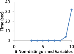
Figure 7: Performance of $\Pi_{2}\mathsf{P}$-complete Algorithms for Non-recursive Programs

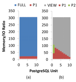
Figure 8: Plan diagram of Felix’s Cost Optimizer

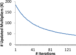
Figure 9: Convergence of Dual Decomposition

D.2 Coverage of the Compiler

Since discovering subtasks as operators is crucial to Felix’s scalability, in this section we test Felix’s compiler. We first evaluate the heuristics we are using for discovering statistical operators given an MLN program. We then evaluate the performance of the $\Pi_{2}\mathsf{P}$-complete algorithm to discovering REF and SYM in non-recursive programs.

Using Heuristics for Arbitrary MLN Programs

While Felix’s compiler can discover all Coref, Labeling, and Classification operators in all programs used in our experiments, we are also interested in how many operators Felix can discover from other programs. To test this, we download the programs that are available on Alchemy’s Web site and manually label operators in these programs. We manually label a set of rules as an operator if this set of rules follows our definition of statistical operators.

We then run Felix’s compiler on these programs and compare the logical plans produced by Felix with our manual labels. We list all programs with manually labeled operators in Table 10. The $x/y$ in each cell of Table  10 means that, among $y$ manually labeled operators, Felix’s compiler discovers $x$ of them.

We can see from Table 10 that Felix’s compiler works well for the programs used in our experiment. Also, Felix works well on discovering classification and labeling operators in Alchemy’s programs. This implies the set of heuristic rules we are using, although not complete, indeed encodes some popular patterns users may use in real world applications. Although some of Alchemy’s programs encode coreference resolution tasks, none of them were labeled as coreference operator. This is because none of these programs explicitly declares the symmetric constraints as hard rules. Therefore, the set of possible worlds decided by the MLN program is different from those decided by the typical “partitioning”-based semantics of coreference operators. How to detect and efficiently implement these “soft-coref” is an interesting topic for future work.

Performance of $\Pi_{2}\mathsf{P}$-complete Algorithm for Non-recursive Programs

In Section 5.3 and Section C.1.1 we show that there are $\Pi_{2}\mathsf{P}$-complete algorithms for annotating REF and SYM properties. Felix implements them. As the intractability is actually inherent in the number of non-distinguished variables, which is usually small, we are interested in understanding the performance of these algorithms.

We start from one of the longest rules found in Alchemy’s Web site which can be annotated as SYM. This rule has 3 non-distinguished variables. We then add more non-distinguished variables and plot the time used for each setting (Figure 7). We can see that Felix uses less than 1 second to annotate the original rule, but exponentially more time when the number of non-distinguished variables grows to 10. This is not surprising due to the exponential complexity of this algorithm. Another interesting conclusion we can draw from Figure 7 is that, as long as the number of non-distinguished variables is less than 10 (which is usually the case in our programs), Felix performs reasonably efficiently.

D.3 Stability of Cost Estimator

In our previous experiments we show that the plan generated by Felix’s cost optimizer contributes to the scalability of Felix. As the optimizer needs to estimate several parameters before performing any predictions, we are interested in the sensitivity of our current optimizer to the estimation errors of these parameters.

The only two parameters used in Felix’s optimizer are 1) the cost (in PostgreSQL’s unit) of fetching one page from the disk and 2) the ratio of the speed between fetching one page from the memory and fetching one page from the disk. We test all combined settings of these two parameters ($\pm 100\%$ of the estimated value) and draw the plan diagram of two queries in Figure 8. We represent different execution plans with different colors. For each point $(x,y)$ in the plan diagram, the color of that point represents which execution plan the compiler chooses if the PostgreSQL’s unit equals $x$ and memory/IO ratio equals $y$.

For those queries not shown in Figure 8, Felix produces the same plan for each tested parameter combination. For queries shown in Figure 8, we can see Felix is robust for parameter mis-estimation. Actually, all the plans shown in Figure 8 are close to optimal, which implies that in our experiments Felix’s cost optimizer avoids the selection of “extremely bad” plans even under serious mis-estimation of parameters.

D.4 Convergence of Dual Decomposition

Felix implements an iterative approach for dual decomposition. One immediate question is how many iterations do we need before the algorithm converges?.

To gain some intuitions, we run Felix on the DBLife data set for a relative long time and record the number of updated Lagrangian multipliers of each iteration. We use constant step size $\lambda=0.9$. As shown in Figure 9, even after more than 130 iterations, the Lagrangian multipliers are still under heavy updates. However, on the ENRON-R dataset, we observed that the whole process converges after the first several iterations! This implies that the convergence of our operator-based framework depends on the underlying MLN program and the size of the input data. It is interesting to see how different techniques on dual decomposition and gradient methods can alleviate this convergence issue, which we leave as future work.

Fortunately, we empirically find that in all of our experiments, taking the result from the first several iterations is often a reasonable trade-off between time and quality – all P/R curves in the previous experiments are generated by taking the last iteration within 3000 seconds and we already get significant improvements compared to baseline solutions. In Felix, to allow users to directly trade-off between quality and performance, we provide two modes: 1) Only run the first iteration and flush the result immediately; and 2) Run the number of iterations specified by the user. It is an interesting direction to explore the possibility of automatically selecting parameters for dual decomposition.

References

- [1] S. Abiteboul and R. Hull. Data functions, datalog and negation. In SIGMOD, 1988.
- [2] S. Abiteboul, R. Hull, and V. Vianu. Foundations of Databases. Addison Wesley, 1995.
- [3] N. Ailon, M. Charikar, and A. Newman. Aggregating inconsistent information: Ranking and clustering. JACM, 2008.
- [4] D. Andrzejewski, L. Livermore, X. Zhu, M. Craven, and B. Recht. A framework for incorporating general domain knowledge into latent Dirichlet allocation using first-order logic. IJCAI, 2011.
- [5] A. Arasu, C. Ré, and D. Suciu. Large-scale deduplication with constraints using Dedupalog. In ICDE 2009.
- [6] D. Bertsekas and J. Tsitsiklis. Parallel and Distributed Computation: Numerical Methods. Prentice-Hall, 1989.
- [7] S. Boyd and L. Vandenberghe. Convex Optimization. Cambridge University Press, New York, 2004.
- [8] A. Carlson, J. Betteridge, B. Kisiel, B. Settles, E. Hruschka Jr, and T. Mitchell. Toward an architecture for never-ending language learning. In AAAI, 2010.
- [9] A. Chandra and P. Merlin. Optimal implementation of conjunctive queries in relational data bases. In STOC, 1977.
- [10] S. Chaudhuri and M. Vardi. On the complexity of equivalence between recursive and nonrecursive datalog programs. In PODS, 1994.
- [11] R. Chirkova, C. Li, and J. Li. Answering queries using materialized views with minimum size. VLDB Journal, 2006.
- [12] P. DeRose, W. Shen, F. Chen, Y. Lee, D. Burdick, A. Doan, and R. Ramakrishnan. DBLife: A community information management platform for the database research community. In CIDR 2007.
- [13] P. Domingos et al. http://alchemy.cs.washington.edu/.
- [14] W. Fan, S. Ma, Y. Hu, J. Liu, and Y. Wu. Propagating functional dependencies with conditions. PVLDB, 2008.
- [15] Y. Fang and K. Chang. Searching patterns for relation extraction over the web: rediscovering the pattern-relation duality. In WSDM, 2011.
- [16] I. Fellegi and A. Sunter. A theory for record linkage. Journal of the American Statistical Association, 1969.
- [17] D. Ferrucci, E. Brown, J. Chu-Carroll, J. Fan, D. Gondek, A. Kalyanpur, A. Lally, J. Murdock, E. Nyberg, J. Prager, et al. Building Watson: An overview of the DeepQA project. AI Magazine, 31(3):59–79, 2010.
- [18] N. Friedman, L. Getoor, D. Koller, and A. Pfeffer. Learning probabilistic relational models. In IJCAI, 1999.
- [19] H. Ji, R. Grishman, H. Dang, K. Griffitt, and J. Ellis. Overview of the tac 2010 knowledge base population track. Proc. TAC2010, 2010.
- [20] J. K. Johnson, D. M. Malioutov, and A. S. Willsky. Lagrangian relaxation for map estimation in graphical models. CoRR, abs/0710.0013, 2007.
- [21] G. Kasneci, M. Ramanath, F. Suchanek, and G. Weikum. The YAGO-NAGA approach to knowledge discovery. SIGMOD Record, 37(4):41–47, 2008.
- [22] H. Kautz, B. Selman, and Y. Jiang. A general stochastic approach to solving problems with hard and soft constraints. The Satisfiability Problem: Theory and Applications, 1997.
- [23] A. Klug. On conjunctive queries containing inequalities. J. ACM, 1988.
- [24] J. Lafferty, A. McCallum, and F. Pereira. Conditional random fields: Probabilistic models for segmenting and labeling sequence data. In ICML, 2001.
- [25] B. Liu, L. Chiticariu, V. Chu, H. Jagadish, and F. Reiss. Automatic rule refinement for information extraction. VLDB, 2010.
- [26] A. McCallum, K. Schultz, and S. Singh. Factorie: Probabilistic programming via imperatively defined factor graphs. In NIPS, 2009.
- [27] E. Michelakis, R. Krishnamurthy, P. Haas, and S. Vaithyanathan. Uncertainty management in rule-based information extraction systems. In SIGMOD, 2009.
- [28] B. Milch, B. Marthi, S. Russell, D. Sontag, D. Ong, and A. Kolobov. BLOG: Probabilistic models with unknown objects. In IJCAI, 2005.
- [29] N. Nakashole, M. Theobald, and G. Weikum. Scalable knowledge harvesting with high precision and high recall. In WSDM, 2011.
- [30] F. Niu, C. Ré, A. Doan, and J. Shavlik. Tuffy: Scaling up statistical inference in Markov logic networks using an RDBMS. In VLDB 2011.
- [31] D. Olteanu, J. Huang, and C. Koch. Sprout: Lazy vs. eager query plans for tuple-independent probabilistic databases. In ICDE, 2009.
- [32] H. Poon and P. Domingos. Joint inference in information extraction. In AAAI 2007.
- [33] R. Ramakrishnan and J. Ullman. A survey of deductive database systems. J. Logic Programming, 1995.
- [34] M. Richardson and P. Domingos. Markov logic networks. Machine Learning, 2006.
- [35] S. Riedel. Cutting Plane MAP Inference for Markov Logic. In SRL 2009.
- [36] N. Rizzolo and D. Roth. Learning based Java for rapid development of NLP systems. Language Resources and Evaluation, 2010.
- [37] A. M. Rush, D. Sontag, M. Collins, and T. Jaakkola. On dual decomposition and linear programming relaxations for natural language processing. In EMNLP, 2010.
- [38] H. Schmid. Improvements in part-of-speech tagging with an application to German. NLP Using Very Large Corpora, 1999.
- [39] J. Seib and G. Lausen. Parallelizing datalog programs by generalized pivoting. In PODS, 1991.
- [40] P. Sen, A. Deshpande, and L. Getoor. PrDB: Managing and exploiting rich correlations in probabilistic databases. J. VLDB, 2009.
- [41] A. Shukla, P. Deshpande, and J. Naughton. Materialized view selection for multidimensional datasets. In VLDB, 1998.
- [42] P. Singla and P. Domingos. Lifted first-order belief propagation. In AAAI, 2008.
- [43] F. Suchanek, M. Sozio, and G. Weikum. SOFIE: A self-organizing framework for information extraction. In WWW, 2009.
- [44] M. Theobald, M. Sozio, F. Suchanek, and N. Nakashole. URDF: Efficient Reasoning in Uncertain RDF Knowledge Bases with Soft and Hard Rules. MPI Technical Report, 2010.
- [45] J. Ullman. Implementation of logical query languages for databases. TODS, 1985.
- [46] M. Wainwright and M. Jordan. Graphical Models, Exponential Families, and Variational Inference. Now Publishers, 2008.
- [47] D. Wang, M. Franklin, M. Garofalakis, J. Hellerstein, and M. Wick. Hybrid in-database inference for declarative information extraction. In SIGMOD, 2011.
- [48] G. Weikum and M. Theobald. From information to knowledge: Harvesting entities and relationships from web sources. In PODS, 2010.
- [49] D. Weld, R. Hoffmann, and F. Wu. Using Wikipedia to bootstrap open information extraction. SIGMOD Record, 2009.
- [50] M. Wick, A. McCallum, and G. Miklau. Scalable probabilistic databases with factor graphs and mcmc. VLDB, 2010.
- [51] L. Wolsey. Integer Programming. Wiley, 1998.
- [52] J. Zhu, Z. Nie, X. Liu, B. Zhang, and J. Wen. Statsnowball: A statistical approach to extracting entity relationships. In WWW, 2009.