Multistep shell model description of spin-aligned neutron-proton pair coupling

Abstract

The recently proposed spin-aligned neutron-proton pair coupling scheme is studied within a non-orthogonal basis in term of the multistep shell model. This allows us to identify simultaneously the roles played by other configurations such as the normal pairing term. The model is applied to four-, six- and eight-hole $N=Z$ nuclei below the core ¹⁰⁰Sn.

Many features in nuclear structure physics can be understood in term of the seniority coupling scheme, which was first introduced in atomic physics by Racah [1]. This scheme showed to be extremely useful for the classification of nuclear states in the $jj$-scheme [2, 3, 4], particularly in semimagic nuclei with only one type of nucleons. The lowest-seniority pair (with $v=0$) has nothing special from a coupling point of view since the nuclear state can then be constructed in a variety of equivalent ways through other pairs. In particular, the aligned like-nucleon pair coupling was proposed in Ref. [5], which may manifest itself from the energy differences of mirror nuclei [6]. The driving force behind the dominance of seniority coupling is the strong pairing interaction between like particles.

The neutron-proton ($np$) correlation breaks the seniority symmetry in a major way. Correspondingly, the wave function is a mixture of many components with different seniority quantum numbers. It is not clear yet how this kind of states can be classified in the $jj$-scheme. The stretch scheme, which corresponds to the maximally aligned intrinsic angular momentum, was proposed in the 1960s to describe the rotational-like spectra of open-shell nuclei [7, 8]. But now it is widely accepted that a proper description of deformation involves the mixture of different orbitals.

The low-lying yrast states in ${}^{92}_{46}$Pd were recently reported [9]. This is the heaviest $N=Z$ nucleus with measured spectrum so far. It was suggested that in this nucleus, as well as in neighboring nuclei like ⁹⁶Cd, the properties of the low-lying states can be largely described in a single $0g_{9/2}$ shell [10, 11]. Furthermore, it was proposed that the low-lying yrast states in these $N=Z$ nuclei can be classified by a spin-aligned $np$ pair coupling scheme [9, 10]. That is, the ground state wave functions do not consist mainly of pairs of neutrons ($\nu\nu$) and protons ($\pi\pi$) coupled to zero angular momenta, but rather of isoscalar $np$ pairs ($\nu\pi$) coupled to the maximum angular momentum $J$, which in the shell $0g_{9/2}$ is $J=9$ [9, 10]. A detailed shell-model analysis of the spin-aligned $np$ pair coupling was performed in Ref. [10]. This shell model calculation was done in the standard fashion of using as representation the tensorial product of neutron times proton degrees of freedom, thus easily takes into account the Pauli principle. The drawback with this representation is that it is not straightforward to realize that the states are mainly determined by $np$ pair degrees of freedom. This can only be done by projecting the shell model wave function into the particular $np$ component one wishes by using two-particle coefficients of fractional parentage. This calculation becomes rather involved for systems with more than three pairs. Moreover, it does not allow one to study simultaneously the competing effects of different $np$ pairs, which requires a large amount of independent projections. A similar calculation was done in Ref. [11] for the two-pair case, just confirming the coupling scheme mentioned above. For systems with three and four pairs, the interacting boson model was applied through the boson mapping of the aligned $np$ pair [11].

In this Letter we will show that a suitable representation to study simultaneously different partitions of a system consisting of many $np$ excitations is the multistep shell model method (MSM) [12]. In this method one solves the shell-model equation in several steps. In the first step one constructs the two-particle states. In the second step one proceed by solving the three- or four-particle states in terms of the two-particle states calculated in the first step. In our case we will solve the two-neutron plus two-proton system within a non-orthogonal overcomplete basis in terms of the $(\nu\pi)\otimes(\nu\pi)$ excitations at the same time as the $(\nu\nu)\otimes(\pi\pi)$ ones. With the four-particle system thus evaluated, we will proceed to evaluate the six-particle system in terms of the coupling of the four-particle and two-particle states. For the eight-particle system one can choose the MSM basis such that it consists of the products of the four-particle states in the form $(\nu\pi)\otimes(\nu\pi)$. Systems with more pairs can be described in the same fashion in successive steps.

The MSM treatment of four and six identical particles was performed in Ref. [12]. Although the formalism to be used here is similar, the present calculation is even more challenging due to the presence of both neutron and proton degrees of freedom. In the case of identical particles the MSM basis is overcomplete mainly because it violate the Pauli principle. In our case the overcompleteness of the basis is even more severe since our basis elements may count twice the same states besides violations of the Pauli principle. For instance, in the two-pair case the basis elements $(\nu\nu)\otimes(\pi\pi)$ and $(\nu\pi)\otimes(\nu\pi)$ may be proportional to each other (see, also, Refs. [10, 11]). The overcounting thus occurring is a result of describing the $np$ and like-particle excitations at the same time. In the MSM this complication is overcome by evaluating the overlap matrix from which an orthonormal set of states can be constructed. This can be a very time consuming procedure for systems with more than two pairs.

We will use the Greek letter $\gamma_{n}$ to label the $n$-particle $np$ states. Since we will only consider cases with equal number of neutrons and protons outside a closed shell, $n$ will be an even number. A $m$-proton ($m$-neutron) state will be labelled by $\alpha_{m}$ ($\beta_{m}$). Therefore the $np$ states will be $|\gamma_{2}\rangle=P^{+}(\gamma_{2})|0\rangle$ where the $np$ creation operator is $P^{+}(\gamma_{2})=\sum_{i,p}X(ip;\gamma_{2})c^{+}_{i}c^{+}_{p}$ and $c^{+}_{i}$ ($c^{+}_{p}$) is the neutron (proton) single-particle creation operator. In the same fashion the two-proton (two-neutron) creation operator will be denoted as $P^{+}(\alpha_{2})$ ($P^{+}(\beta_{2})$) (c.f., Eq. (9) of Ref. [12]). The four-particle state, $|\gamma_{4}\rangle=P^{+}(\gamma_{4})|0\rangle$, is

$$P^{+}(\gamma_{4}) = \sum_{\alpha_{2},\beta_{2}}X(\alpha_{2}\beta_{2};\gamma_{4})P^{+}(\alpha_{2})P^{+}(\beta_{2})$$ (1)

$$+ \sum_{\gamma_{2}\leq\gamma_{2}^{\prime}}X(\gamma_{2}\gamma_{2}^{\prime};\gamma_{4})P^{+}(\gamma_{2})P^{+}(\gamma_{2}^{\prime}),$$

where all possible like-particle and $np$ pairs are taken into account. Since the number of MSM basis vectors is larger than the dimension of the shell model space, the wave function amplitudes $X$ are not well defined in our case and, therefore, they are not meaningful physically. The meaningful quantities are the projections of the basis vectors upon the physical vector, which we denote as

$$F(\alpha_{2}\beta_{2};\gamma_{4}) = \langle\gamma_{4}|P^{+}(\alpha_{2})P^{+}(\beta_{2})|0\rangle,$$

$$F(\gamma_{2}\gamma_{2}^{\prime};\gamma_{4}) = \langle\gamma_{4}|P^{+}(\gamma_{2})P^{+}(\gamma_{2}^{\prime})|0\rangle.$$ (2)

The orthonormality condition now reads

$$\delta_{\gamma_{4}\gamma_{4}^{\prime}} = \sum_{\alpha_{2},\beta_{2}}X(\alpha_{2}\beta_{2};\gamma_{4})F(\alpha_{2}\beta_{2};\gamma_{4}^{\prime})$$ (3)

$$+ \sum_{\gamma_{2}\leq\gamma_{2}^{\prime}}X(\gamma_{2}\gamma_{2}^{\prime};\gamma_{4})F(\gamma_{2}\gamma_{2}^{\prime};\gamma_{4}).$$

The norm of the MSM basis $|\gamma_{2}\gamma_{2}^{\prime}\rangle$ $=$ $P^{+}(\gamma_{2})P^{+}(\gamma_{2}^{\prime})|0\rangle$, i.e., $N(\gamma_{2}\gamma_{2}^{\prime};\gamma_{4})=\sqrt{\langle\gamma_{2}\gamma_{2}^{\prime}|\gamma_{2}\gamma_{2}^{\prime}\rangle}$, may not be unity. Therefore the interesting quantity is not the projection $F$ but rather the cosine of the angle between the basis vector and the physical vector, i.e., $\cos(\phi)=x$ and

$$x(\gamma_{2}\gamma_{2}^{\prime};\gamma_{4})=F(\gamma_{2}\gamma_{2}^{\prime};\gamma_{4})/N(\gamma_{2}\gamma_{2}^{\prime};\gamma_{4}).$$ (4)

If we would have taken as basis elements the complete set of orthonormal states $\{P^{+}(\alpha_{2})P^{+}(\beta_{2})|0\rangle\}$ (which is the standard shell model basis as used in Ref. [10]) then the second term in Eq. (3) would not have appeared and one would have obtained $X(\alpha_{2}\beta_{2};\gamma_{4})=x^{*}(\alpha_{2}\beta_{2};\gamma_{4})$, as expected in an orthonormal basis. One thus sees that the advantage of the MSM basis is that one can extract the physical structure of the calculated states just by examining the quantity $x$.

For the six-particle case we will use the MSM partition of two- times four-particles, as it was done in Ref. [12] for systems with six like particles. Thus the corresponding wave function will be $|\gamma_{6}\rangle=P^{+}(\gamma_{6})|0\rangle$, where

$$P^{+}(\gamma_{6})=\sum_{\gamma_{2},\gamma_{4}}X(\gamma_{2}\gamma_{4};\gamma_{6})P^{+}(\gamma_{2})P^{+}(\gamma_{4}).$$ (5)

As before, we will evaluate the projection of the basis vectors upon the physical vectors, i.e., $F(\gamma_{2}\gamma_{4};\gamma_{6})$, and the corresponding cosine function $x$. In this six-particle case one can also view the MSM basis elements as the direct tensorial product of three pairs. This is a unique feature of the MSM. The projection of such a MSM basis upon the physical vector is,

$$F(\gamma_{2}\gamma_{2}^{\prime}\gamma_{2}^{\prime\prime};\gamma_{6}) = \langle\gamma_{6}|P^{+}(\gamma_{2})P^{+}(\gamma_{2}^{\prime})P^{+}(\gamma_{2}^{\prime\prime})|0\rangle$$ (6)

$$= \sum_{\gamma_{4}}F(\gamma_{2}\gamma_{4};\gamma_{6})F(\gamma_{2}^{\prime}\gamma_{2}^{\prime\prime};\gamma_{4}),$$

from which one can evaluate the norm as $N^{2}(\gamma_{2}\gamma_{2}^{\prime}\gamma_{2}^{\prime\prime};\lambda)=\sum_{\gamma_{6}(\lambda)}|F(\gamma_{2}\gamma_{2}^{\prime}\gamma_{2}^{\prime\prime};\gamma_{6})|^{2}$, where $\lambda$ is the total angular momentum of the state and the sum runs over all physical states $\gamma_{6}$ with angular momentum $\lambda$. The cosine of the angle between a MSM basis and the physical state is

$$x(\gamma_{2}\gamma_{2}^{\prime}\gamma_{2}^{\prime\prime};\gamma_{6})=F(\gamma_{2}\gamma_{2}^{\prime}\gamma_{2}^{\prime\prime};\gamma_{6})/N(\gamma_{2}\gamma_{2}^{\prime}\gamma_{2}^{\prime\prime};\lambda).$$ (7)

We will describe the eight-particle states as $|\gamma_{8}\rangle$ = $P^{+}(\gamma_{8})|0\rangle$, where $P^{+}(\gamma_{8})$ = $\sum_{\gamma_{4}\leq\gamma_{4}^{\prime}}X(\gamma_{4}\gamma_{4}^{\prime};\gamma_{8})P^{+}(\gamma_{4})P^{+}(\gamma_{4}^{\prime})$. Proceeding as above we will also evaluate the cosine of the angle between $|\gamma_{8}\rangle$ and all the possible four-pair states that can be formed.

It is important to point out that for any MSM basis element $|b_{n}\rangle$ corresponding to the $n$-particle system it is $\sum_{\gamma_{n}}x^{2}(b_{n},\gamma_{n})$=1. This is because the vectors $|\gamma_{n}\rangle$, which are eigenvectors of the $n$-particle Shell Model Hamiltonian, form an orthonormal (complete) set. Therefore the cosine $x(b_{n},\gamma_{n})$ is the probability of the state $|\gamma_{n}\rangle$ occupying the basis state $|b_{n}\rangle$.

We will apply the method to study the spin-aligned $np$ pair coupling scheme [9, 10]. We will restrict our calculations to the single $0g_{9/2}$ shell with the interaction matrix elements taken from Ref. [10]. But it should be emphasized that the formalism proposed in the present work can be naturally generalized to systems with many shells.

In the cases of ⁹⁶Cd and ⁹²Pd the low-lying spectra are determined by the isoscalar and strongly attractive matrix element $\langle(g_{9/2})^{2};9|V|(g_{9/2})^{2};9\rangle$ [10], which corresponds to the maximally aligned $np$ pair configuration. The extend to which this determines the spectrum can be deemed by the evolution of the calculated levels as a function of the variations of that matrix element. Calling $V_{9}(\delta)=V_{9}(0)(1+\delta)$ it is found that as $V_{9}(\delta)\rightarrow 0$ the spectrum tends to have a seniority-like form. At the other extreme, approaching $\delta$=1, a tendency towards a vibrational-like spectrum seems to take place [10]. This is not surprising since, as also seen below, all low-lying yrast states in both nuclei are isoscalar $np$ pair excitations [10].

The MSM provides in a straightforward fashion the structure of the states in terms of all possible configurations. Thus, in Fig. 1 we show the main values of the probabilities $x^{2}$ (Eq. (4)), as a function of the controlling parameter $\delta$, for the ground state and first $2^{+}$ state of ⁹⁶Cd. The striking feature in this figure is that the spectrum for $\delta$=0 is dominated by the isoscalar configuration $((\nu\pi)_{9})^{2}$. Moreover, one sees that as $V_{9}(\delta)$ becomes more attractive ($\delta\rightarrow 1$) the pairing state becomes less and less relevant while the importance of other isoscalar components increases. This feature is even more remarkable for the state $2^{+}_{1}$, where the spin-aligned $np$ pair coupling $((\nu\pi)_{9})^{2}$ dominates the wave function for all values of $\delta$ shown in the figure.

Figure 1: (Color online) Upper: Coefficients $x^{2}$ corresponding to the wave function of the ground state of ⁹⁶Cd as a function of the controlling parameter $\delta$ (see text). The labels indicate 1: $|((\nu\pi)_{9})^{2};0\rangle$; 2: $|(\nu\nu)_{0}(\pi\pi)_{0};0\rangle$; 3: $|((\nu\pi)_{1})^{2};0\rangle$; 4: $|(\nu\nu)_{2}(\pi\pi)_{2};0\rangle$. Lower: Same as the upper panel but for the first $2^{+}$ state. The labels correspond to 1: $|((\nu\pi)_{9})^{2};2\rangle$; 2: $|(\nu\pi)_{0}(\nu\pi)_{2};2\rangle$. Only configurations with $x^{2}>0.4$ are shown for simplicity.

One may wonder whether the pairing mode $|(\nu\nu)_{0}(\pi\pi)_{0};0\rangle$, which does not dominate the ground state in ⁹⁶Cd, would be located as a state $0^{+}$ higher up in the spectrum. However, this is not the case, as can be seen from Table 1 where we listed the main components of the lowest-lying states in ⁹⁶Cd for different total angular momenta. Rather it is distributed throughout the spectrum. In contrast, the isoscalar aligned mode $|((\nu\pi)_{9})^{2};I\rangle$ is mainly concentrated in the yrast states. It may seem weird that these two modes produce different results since they may be related to each other just by an exchange of neutrons and protons. But they are not the same, as shown by the angle $\phi$ between them which gives $\cos(\phi)$=0.62, i.e., $\phi=52^{\circ}$. It is also interesting to notice that the norm of the aligned state is $\langle((\nu\pi)_{9})^{2};0|((\nu\pi)_{9})^{2};0\rangle=2.00001$, which shows that the influence of the Pauli principle upon $|((\nu\pi)_{9})^{2};0\rangle$ is negligible and, therefore, it represents virtually a bosonic mode (see also Ref. [11]).

Table 1: Leading configurations in the first five states of ⁹⁶Cd for a given total angular momentum $I$.

	$I=0$			$I=2$			$I=4$			$I=6$
n	Configuration	$|x|$		Configuration	$|x|$		Configuration	$|x|$		Configuration	$|x|$
1	$(\nu\pi)_{9}\otimes(\nu\pi)_{9}$	0.96		$(\nu\pi)_{9}\otimes(\nu\pi)_{9}$	0.99		$(\nu\pi)_{9}\otimes(\nu\pi)_{9}$	0.97		$(\nu\pi)_{9}\otimes(\nu\pi)_{9}$	0.84
2	$(\nu\pi)_{5}\otimes(\nu\pi)_{5}$	0.88		$(\nu\pi)_{8}\otimes(\nu\pi)_{9}$	0.92		$(\nu\pi)_{8}\otimes(\nu\pi)_{9}$	0.93		$(\nu\pi)_{7}\otimes(\nu\pi)_{9}$	0.60
3	$(\nu\pi)_{0}\otimes(\nu\pi)_{0}$	0.77		$(\nu\pi)_{7}\otimes(\nu\pi)_{9}$	0.94		$(\nu\pi)_{7}\otimes(\nu\pi)_{9}$	0.90		$(\nu\nu)_{0(6)}\otimes(\pi\pi)_{6(0)}$	0.94
4	$(\nu\pi)_{3}\otimes(\nu\pi)_{3}$	0.91		$(\nu\pi)_{7}\otimes(\nu\pi)_{8}$	0.82		$(\nu\pi)_{5}\otimes(\nu\pi)_{9}$	0.90		$(\nu\nu)_{2(6)}\otimes(\pi\pi)_{6(2)}$	0.65
5	$(\nu\pi)_{4}\otimes(\nu\pi)_{4}$	0.80		$(\nu\pi)_{5}\otimes(\nu\pi)_{7}$	0.64		$(\nu\pi)_{6}\otimes(\nu\pi)_{9}$	0.92		$(\nu\nu)_{2(6)}\otimes(\pi\pi)_{6(2)}$	0.84

The calculated spectrum of the odd-odd nucleus ${}^{94}_{47}$Ag is shown in Fig. 2, where we have grouped the levels according to their isospin. There are only two states which have been measured in this case [13], namely the $0^{+}$ ground state and a state $21^{+}$ at 6.67 MeV. These states are in reasonable agreement with experiment and coincide with previous shell model calculations [14]. The strong influence of the aligned isoscalar matrix element $V_{9}$ upon the $T=0$ states can be inferred from the figure, where it is seen that the energies of $T=0$ states are much more sensitive to the controlling parameter $\delta$ than those with $T=1$.

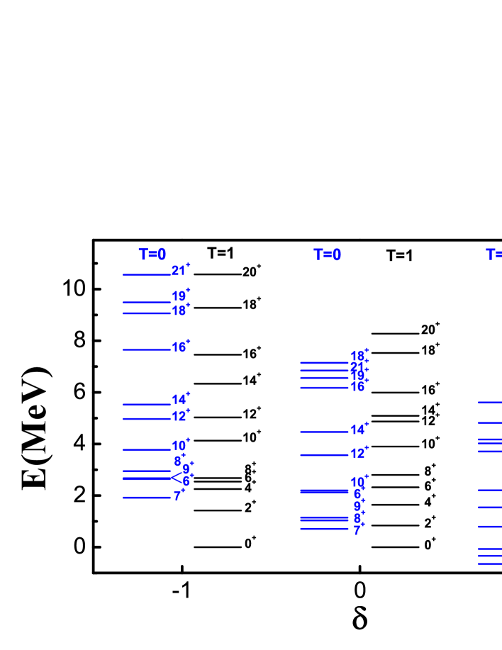
Figure 2: (Color online) Shell model spectra of ⁹⁴Ag calculated in the ${0g_{9/2}}$ shell as a function of the controlling parameter $\delta$.

Figure 3: (Color online) Upper: Coefficients $x^{2}$ corresponding to the wave function of ⁹⁴Ag ($0^{+}_{1}$) as a function of $\delta$. The labels indicate 1: $|(\nu\pi)_{0}(\nu\pi)_{9}(\nu\pi)_{9});0\rangle$; 2: $|(\nu\pi)_{0}(\nu\nu)_{2}(\pi\pi)_{2});0\rangle$; 3: $|(\nu\pi)_{1}(\nu\nu)_{8}(\pi\pi)_{8});0\rangle$; 4: $|(\nu\pi)_{0}(\nu\pi)_{0}(\nu\pi)_{0});0\rangle$; 5: $|(\nu\pi)_{0}(\nu\pi)_{5}(\nu\pi)_{5});0\rangle$; 6: $|(\nu\pi)_{0}(\nu\nu)_{0}(\pi\pi)_{0});0\rangle$. Lower: Same as the upper panel but for the $7^{+}_{1}$ state. The labels indicate 1: $|(\nu\pi)_{0}(\nu\pi)_{9}(\nu\pi)_{9});7\rangle$; 2: $|(\nu\pi)_{7}(\nu\nu)_{0}(\pi\pi)_{0});0\rangle$; 3: $|(\nu\pi)_{7}(\nu\pi)_{0}(\nu\pi)_{0});7\rangle$.

The $T=0$ states in ⁹⁴Ag are specially interesting because in this case the MSM basis vector consisting of the three $9^{+}$ isoscalar aligned states is not hindered by any symmetry (recall that only states with total isospin $T=0$ can be coupled from the isoscalar $np$ pairs). Indeed we found that most of the yrast levels in Fig. 2, except the $16^{+}_{1}$ and $18^{+}_{1}$ states, are mainly built by the isoscalar aligned $np$ pairs. As an example, in the lower panel of Fig. 3 we present the the probabilities $x^{2}$ for main components of the $7^{+}_{1}$ state of ⁹⁴Ag, which is calculated to be the lowest $T=0$ state, as a function of the controlling parameter $\delta$.

It is seen from Fig. 2 that at $\delta=0$ the ground state of ⁹⁴Ag carries $T=1$. It may thus seem that in odd-odd system the isovector pairing mode retakes its predominance. We found that this is not the case by analyzing the ground state wave function in terms of the tensor product of three pairs, as can be seen from the upper panel of Fig. 3. The most important configuration consists of the spin-aligned $np$ pair state $|(\nu\pi)_{9}(\nu\pi)_{9});0\rangle$ that was dominant in ⁹⁶Cd and the other possible configuration, i.e., the isovector state $|(\nu\pi)_{0}\rangle$. In fact the low-lying $T=1$ states here have the same origin as the corresponding $T=1$ states in ⁹⁴Cd. One sees that in this odd-odd six-particle case the probabilities of the ground state occupying different basis states are larger than in ⁹⁶Cd, Fig. 1. This is not surprising since for systems with more than two pairs there are many nearly equivalent combinations that can be built in the same fashion.

In the analysis of eight-particle systems like ⁹²Pd we choose as MSM basis the partition $|\gamma_{4}\gamma_{4}^{\prime};\gamma_{8}\rangle$. In this case the MSM basis is highly overcomplete. For instance there are 36 shel-model $0^{+}$ states while the corresponding MSM dimension is 915. Within this basis we calculated in Table 2 the quantities $x$, i.e., the cosines of the angles between the vectors $|\gamma_{8}\rangle$ and all the possible vectors that can be formed by the coupling of four pairs. Since many combinations are similar to each other there is not a value of $x$ which is significantly larger than the others. But one finds, again, that for the ground state of ⁹²Pd the most important MSM configuration is the one corresponding to the four $9^{+}$ aligned pairs. The second one is a combination of two aligned $9^{+}$ states and the normal pairing states. This is expected since in the two-pair case of ⁹⁶Cd the second largest component is the normal pairing term. An important feature in this case is that for the pairing state it is $x^{2}(\alpha_{2}=0^{+},\beta_{2}=0^{+}\alpha_{2}^{\prime}=0^{+}\beta_{2}^{\prime}=0^{+};\gamma_{8}=0^{+}_{1})$ = 0.46. This is a relatively small number. Indeed it occupies the 10th place in order of importance. This reflects, once again, the dominance of the aligned configuration in this nuclear region.

Table 2: Configurations with the largest probabilities for the state ⁹²Pd($0^{+}_{1}$) corresponding to the tensorial products of different two-particle states (upper) and four-particle states (lower).

Configuration	$x^{2}$
$|\gamma_{2}=9^{+}\gamma_{2}^{\prime}=9^{+}\gamma_{2}^{\prime\prime}=9^{+}\gamma_{2}^{\prime\prime\prime}=9^{+}\rangle$	0.85
$|\gamma_{2}=9^{+}\gamma_{2}^{\prime}=9^{+}\alpha_{2}=0^{+}\beta_{2}=0^{+}\rangle$	0.76
$|\gamma_{2}=8^{+}\gamma_{2}^{\prime}=1^{+}\alpha_{2}=0^{+}\beta_{2}=8^{+}\rangle$	0.56
$|\gamma_{2}=8^{+}\gamma_{2}^{\prime}=1^{+}\alpha_{2}=8^{+}\beta_{2}=0^{+}\rangle$	0.56
$|\gamma_{2}=1^{+}\gamma_{2}^{\prime}=1^{+}\alpha_{2}=0^{+}\beta_{2}=0^{+}\rangle$	0.52

Summarizing, we have in this paper extended the MSM method proposed in Ref. [12] to incorporate both neutron and proton degrees of freedom and applied it to study the recently proposed spin-aligned $np$ pair coupling scheme. We have applied the method to analyze four-, six- and eight-hole states in $N=Z$ nuclei below the core ¹⁰⁰Sn. The calculations were performed within the restricted $0g_{9/2}$ shell for simplicity. But this work opens the way for even more challenging calculations, involving many particles and/or many shells. It would also allow one to truncate the shell model basis in terms of spin-aligned $np$ pairs or other coupling schemes.

This work was supported by the Swedish Research Council (VR) under grant Nos. 623-2009-7340 and 2010-4723. Z.X. is supported in part by the China Scholarship Council under grant No. 2008601032.

References

- [1] G. Racah, Phys. Rev. 63 (1943) 367.
- [2] M. G. Mayer, Phys. Rev. 78 (1950) 22.
- [3] B. H. Flowers, Proc. R. Soc. A 212 (1952) 248.
- [4] I. Talmi, Simple Models of Complex Nuclei (Harwood Academic Publishers, Chur, Switzerland, 1993).
- [5] H.T. Chen, D.H. Feng, and C.L. Wu, Phys. Rev. Lett. 69 (1992) 418.
- [6] S. M. Lenzi et al., Phys. Rev. Lett. 87 (2001) 122501.
- [7] M. Danos and V. Gillet, Phys. Rev. Lett. 17 (1966) 703.
- [8] M. Danos and V. Gillet, Phys. Rev. 161 (1967) 1034.
- [9] B. Cederwall et al., Nature 469 (2011) 68.
- [10] C. Qi, T. Bäck, J. Blomqvist, B. Cederwall, R. J. Liotta and R. Wyss, arXiv: 1101.4046, Phys. Rev. C (R), in press.
- [11] S. Zerguine and P. Van Isacker, Phys. Rev. C 83 (2011) 064314.
- [12] R. J. Liotta and C. Pomar, Nucl. Phys. A 362 (1981) 137.
- [13] National Nuclear Data Center (NuDat2.5), Brookhaven National Laboratory at http://www.nndc.bnl.gov/nudat2/.
- [14] M. La Commara et al., Nucl. Phys. A 708 (2002) 167.