Analysis of rolling group therapy data using conditionally autoregressive priors

Abstract

Group therapy is a central treatment modality for behavioral health disorders such as alcohol and other drug use (AOD) and depression. Group therapy is often delivered under a rolling (or open) admissions policy, where new clients are continuously enrolled into a group as space permits. Rolling admissions policies result in a complex correlation structure among client outcomes. Despite the ubiquity of rolling admissions in practice, little guidance on the analysis of such data is available. We discuss the limitations of previously proposed approaches in the context of a study that delivered group cognitive behavioral therapy for depression to clients in residential substance abuse treatment. We improve upon previous rolling group analytic approaches by fully modeling the interrelatedness of client depressive symptom scores using a hierarchical Bayesian model that assumes a conditionally autoregressive prior for session-level random effects. We demonstrate improved performance using our method for estimating the variance of model parameters and the enhanced ability to learn about the complex correlation structure among participants in rolling therapy groups. Our approach broadly applies to any group therapy setting where groups have changing client composition. It will lead to more efficient analyses of client-level data and improve the group therapy research community’s ability to understand how the dynamics of rolling groups lead to client outcomes.

, , and t1Supported in part by NIH/NIAAA Grant R01AA019663. t2Supported in part by NIH/NIDDK Grant R01DK061662. t3Supported in part by NIH/NIAAA Grant R01AA014699.

1 Introduction

1.1 Group therapy

Group therapy is a central treatment modality for behavioral health disorders, such as alcohol and other drug use (AOD) disorders [Kadden et al. (2001); Kadden and Litt (2004); Monti et al. (2002); Crits-Christoph et al. (1999); Wells et al. (1994)] and depression [Thompson et al. (1983); Neimeyer et al. (1989); Robinson, Berman and Neimeyer (1990); Bright, Baker and Neimeyer (1999)]. Most community-based behavioral health treatment is provided in groups. Its therapeutic strengths include group members having opportunities to develop and practice new social skills and behaviors, receiving feedback from other group members, learning from the shared experiences of other group members, and providing a recovery network to clients [Neimeyer et al. (1989); Satterfield (1994)]. Group therapy is especially relevant for treatment providers in light of rising costs, as group therapy has clear economic advantages over individual therapy [Jacobs and Goodman (1989); Bright, Baker and Neimeyer (1999); Monti et al. (2002)]. These advantages are evident in our motivating study, Building Recovery by Improving Goals, Habits and Thoughts (BRIGHT). In BRIGHT, AOD treatment clients with depressive symptoms received group cognitive behavioral therapy (CBT) that was delivered by AOD treatment counselors, rather than psychotherapists. The analytic question we consider in this paper is whether the depressive symptoms of AOD clients decreased while attending group CBT over an 8-week period.

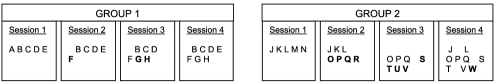
Figure 1: Illustration of client flow under rolling admissions. Each group contains different sets of clients (represented by letters). Bold letters represent new members entering each group.

1.2 Group therapy with rolling admissions

A feature of the group CBT offered in BRIGHT that is shared by many therapy groups offered in other AOD treatment settings is that clients enter group under a rolling (or open) admissions policy. This means that clients are continuously enrolled in group as space permits. Figure 1 illustrates a hypothetical rolling admission policy for two therapy groups (labeled “GROUP 1” and “GROUP 2”), each of which has four sessions. It is important to note the difference between groups and sessions. The two groups in Figure 1 each have four sessions. The sessions in Group 1 are independent of sessions in Group 2 because there is no overlap in the sets of clients who attend the sessions in Group 1 versus Group 2—for example, in Figure 1, clients A–H attend Group 1 and clients J–W attend Group 2. In contrast, the sessions within each group are not independent since clients may attend multiple sessions within each group. For example, clients B, C, D attend all four sessions offered in Group 1. The “rolling” admissions policy is depicted in Figure 1, with new members indicated by boldface font in the first session they attend. While new members join the group, other members leave (e.g., client A left Group 1 after session 1 and was replaced by client F in session 2). This structure induces a complex pattern of interrelatedness among clients. Even though clients A and F in Group 1 never attend the same session, their data could be correlated. One example of this would be if client A were a disruptive client [Center for Substance Abuse Treatment (2005)] who adversely influenced the overall group dynamic in session 1 of Group 1 in such a way that clients B through E would bring that negativity with them to session 2, thus affecting client F’s group experience.

Figure 2: Attendance by clients A–Q for sessions 1–36 in one rolling therapy group in the BRIGHT study. Study modules are separated by dashed vertical lines.

Figure 2 illustrates the actual client attendance patterns for $17$ clients who participated in one of the four rolling cognitive behavioral therapy (CBT) groups in the BRIGHT study. This group included $36$ sessions. Each client (labeled A through Q) was expected to complete $16$ sessions, with $4$ sessions coming from each of four modules (or session themes)—Thoughts, Activities, People, or Substance Abuse—as noted at the top of Figure 2. Modules were offered on a rotating basis, and clients were allowed to enter the group at the start of a new module (e.g., at session 5, 9, 13, 17, 21, 25, or 33). This illustrates the flexibility of treatment delivery afforded by rolling groups in BRIGHT—for example, a client only needed to wait for a new module, rather than an entirely new but closed 16-session group, to start CBT.

Thus, not only are client outcomes correlated within therapy sessions, but they are also correlated across therapy sessions within each therapy group. This is in contrast to the analytically much simpler scenario of “closed” enrollment groups, in which the same set of clients is expected to attend the same set of sessions with no change in membership, such that the correlation in the outcomes for clients in the same closed group could be modeled using a hierarchical model with random terms for each closed therapy group.

1.3 Previous approaches to modeling data from rolling therapy groups

Despite the ubiquity of groups with rolling admissions in practice [Kadden et al. (2001); Kadden and Litt (2004); Monti et al. (2002); Rohsenow et al. (2001, 2004); Davis et al. (2005); Granholm et al. (2005); Center for Substance Abuse Treatment (2005)], very little attention has been devoted to developing appropriate statistical methods for such data. In a review article, the possibility was discussed of using standard hierarchical models that used group as the clustering variable (e.g., Figure 1), but was dismissed because it ignores the complex attendance pattern within the group [Morgan-Lopez and Fals-Stewart (2006)]. Another possibility discussed therein was to break up the group into subgroups in some fashion and use a multiple membership model, but the independence assumption typically invoked for such models was criticized. Perhaps even more frequently, the approach taken in therapy group studies—with rolling or closed groups—is to ignore the group structure altogether [Lee and Thompson (2005); Roberts and Roberts (2005); Bauer, Sterba and Hallfors (2008)].

To date, the only analytic method specifically developed and applied to data collected from clients as they attend rolling group sessions did not explicitly model the correlation among outcomes from clients within a group [Morgan-Lopez and Fals-Stewart (2007)]. Rather, the authors of that study fit models assuming no correlation but adjusted the standard errors to account for possible correlation among clients who attended the same group (not session) using a robust standard error (sandwich) estimator [Liang and Zeger (1986)]. The authors also addressed the potential problem of nonignorable missing data [e.g., Little (1995)] from clients who chose not to attend all sessions by using a pattern mixture model, where patterns depended on latent classes related to number of sessions attended and client characteristics. Morgan-Lopez and Fals-Stewart (2008) found that modeling different missing data (attendance) patterns helped with variance estimation, in that nominal Type 1 error rates were preserved.

However, there are some important limitations to this approach. First, even when nonignorably missing data are a major problem, modeling missing data patterns does not account for the correlation structure depicted in Figures 1 and 2, leading to concerns that even pattern-mixture modeling without accounting for the intra- or inter-session correlation of client outcomes could lead to underestimated variances. Second, using the sandwich estimator is only appropriate in studies with large numbers of rolling groups. The sandwich estimator will only provide a consistent estimate of standard errors of parameter estimates, as the number of therapy groups grows arbitrarily large, and it can be biased when the number of groups is small [Liang and Zeger (1986); Bell and McCaffrey (2002)]. The number of rolling groups is small (as few as 1–4) in many rolling group studies [Kadden et al. (2001); Kadden and Litt (2004); Rohsenow et al. (2001, 2004)]; in the motivating BRIGHT study, there were just four rolling groups. Third, the sandwich estimator only adjusts the standard errors; it does not model the clustering of client outcomes both within and across sessions and does not provide information about the sources of variance. Finally, even in studies with large numbers of rolling groups, relying on the sandwich estimator to adjust for correlation at the group level would be inefficient relative to model-based approaches to directly model the correlation structure attributable to session attendance [Firth (1992)].

1.4 Conditionally autoregressive priors

Given these limitations, we present a novel application of conditionally autoregressive (CAR) priors [Besag, York and Mollié (1991)] for modeling session-level random effects to capture the interrelatedness of client outcomes. CAR priors offer promise for adeptly modeling correlations at the session level that are induced by session attendance patterns. Though a quick glance at Figures 1–2 might suggest that a potentially simpler time series approach might be appropriate, the CAR prior can accommodate alternative scenarios that frequently occur in practice, such as sessions offered at unequally spaced points in time, multiple independent sets of therapy group sessions or “islands” [Hodges, Carlin and Fan (2003)], and flexible definitions of closeness of sessions that cover a broad range of complex scenarios, such as accounting for number of clients shared by sessions or variable lengths of time between sessions.

In this paper we describe the motivating BRIGHT study (Section 2) and present a hierarchical Bayesian CAR model for the BRIGHT data (Section 3). In Section 4 we examine the relative performance of the Bayesian CAR approach versus competing approaches for accounting for the interdependence of client outcomes. We compare these approaches using BRIGHT data to examine whether depressive symptoms decrease during the course of group therapy in Section 5. We conclude by discussing the implications of our method for therapy group data analysis in Section 6.

2 Motivating study: Building Recovery by Improving Goals, Habits and Thoughts (BRIGHT)

The BRIGHT study addressed the question of whether group cognitive behavioral therapy (CBT) improves depressive symptoms when delivered by substance abuse treatment counselors. The goal of the group CBT offered in BRIGHT was to help persons with depressive symptoms manage their depression and feel better. The study occurred at four treatment sites that are part of the Behavioral Health System (BHS) of Los Angeles County, California. BHS is a nonprofit treatment provider and is among the largest publicly funded programs in Los Angeles County.

BHS clients were screened for study eligibility using a two-stage process. First, BHS staff screened clients using the Patient Health Questionnaire [PHQ-9; Kroenke and Spitzer (2002)] 14 days after entering residential treatment. The PHQ-9 is a nine-item self-report measure that assesses the nine depression symptoms from the DSM-IV depression criteria. If clients received a PHQ-9 score indicating mild-to-severe depressive symptoms (i.e., PHQ-9${}\geq 5$), they were asked whether they were interested in being contacted to learn more about the study. A second screening was then conducted to verify that clients had persistent depressive symptoms and thus were eligible for the study by examining whether a second depressive symptom score, the Beck Depression Inventory-II [BDI-II; Beck, Steer and Brown (1996)], indicated mild-to-severe depressive symptoms (BDI-II${}>17$). In addition, clients with bipolar disorder, schizophrenia, or cognitive impairment were ineligible for the study, but clients taking psychotropic medications for other reasons were eligible so long as they had depressive symptoms as indicated by the two-stage screening procedure. Participants were enrolled in the study 3–4 weeks after admission to residential AOD treatment. Seventy-six percent of those entering residential AOD treatment were screened by BHS for depression and 25% of those clients were eligible for the study based on the second screening. For this study, we examined data collected from clients assigned to the group CBT intervention ($n=140$) and analyzed changes in depressive symptoms during the course of group CBT for the $132$ clients who attended at least one group CBT session.

The BRIGHT group therapy consisted of $16$ sessions of group CBT offered over an eight-week period that were organized into four modules of four sessions each. Each module focused on the relationship between depression and a particular aspect of a person’s life: Thoughts, Activities, People, and Substance Use. Research suggests that each module is independently efficacious [Zeiss, Lewinsohn and Munoz (1979)] and does not depend on the material presented in the previous module, thus making the rolling admissions policy reasonable. The four modules over $16$ sessions were offered on a rotating basis, as shown for one rolling group in Figure 2. The CBT group had a rolling admissions policy, as client composition of the group was allowed to change every two weeks. Specifically, clients were able to initiate treatment at the first session of any module, which is graphically depicted for one rolling CBT group in BRIGHT in Figure 2. In session one of each module the cognitive–behavioral treatment model was described and information about depression and its symptoms were provided to the clients.

In all, $245$ group CBT sessions were offered to clients from all four treatment sites. This included $14$ offerings of the $16$-session sequence ($224$ sessions), $20$ additional sessions from the “Thoughts” and “Activities” modules to increase exposure to group CBT for those who joined the rolling group late for three particular $16$-week sequences, and one additional session that followed a long holiday weekend to make up for poor attendance at the regularly scheduled session. These $245$ sessions were divided into four CBT therapy groups having distinct clients; the number of sessions for each of these four groups was 36, 40, 40, and 129.

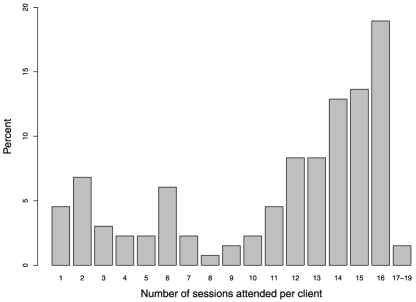
Figure 3: Distribution of the number of sessions attended per client.

The number of sessions attended per client skewed toward more versus fewer sessions (Figure 3). Seventy-three percent of clients attended at least half of the sessions (eight sessions), and $45\%$ attended $13$ or more sessions. Sixty-three percent of clients attended at least one session per module.

3 Hierarchical Bayesian modeling of correlated therapy group session effects

The goal of analyzing the client-level PHQ data collected from clients during the course of group CBT is to estimate client-level change over time. The core analytic model for this is a growth curve model [or longitudinal growth model (LGM) of Laird and Ware (1982)], where there are $i=1,\ldots,n$ clients in the study, $s=1,\ldots,S$ therapy group sessions offered over the course of the study, and $t_{is}$ is the time that has passed since client $i$ entered the therapy group when attending session $s$. Note the difference between $s$ and $t$: $s$ indexes all $S$ sessions offered to all clients, while $t$ ranges from $0$ to the maximum length of time between treatment entry and completion at the client level; in BRIGHT, $t$ ranges from $0$ to $8$ weeks since entry into group. The repeatedly measured PHQ-9 score for client $i$ at session $s$ after attending the group for time $t_{is}$ is denoted by $y_{is}$, and is modeled as

$$y_{is}=\beta_{0}+\beta_{1}t_{is}+\sum_{k=1}^{K}\beta_{k+1}X_{ik}+b_{0i}+b_{1i}t_{is}+\gamma_{s}+\varepsilon_{is},$$ (1)

where baseline covariates, $X_{1},\ldots,X_{K}$, have coefficients $\beta_{2}$ through $\beta_{K+1}$; $\beta_{0}$ is the fixed intercept term; $\beta_{1}$ the mean (fixed effect) rate of change in $y$ for all clients; the random effects growth parameters for client $i$ have distributions $b_{0i}\sim N(0,\sigma^{2}_{0})$ and $b_{1i}\sim N(0,\sigma^{2}_{1})$; $\varepsilon_{is}$ is the observation error with distribution $N(0,\sigma^{2}_{\varepsilon})$; and the session-specific random effects, $\gamma_{s}$, are included in the model to capture session-specific variation in client outcomes. The session-level random effects, $\gamma_{s}$, are modeled using a convolution prior [Besag, York and Mollié (1991)]:

$$\gamma_{s}=u_{s}+\nu_{s},$$ (2)

modeling the random effect of session $s$ as having both structured and unstructured components to accommodate not only structured, systematic correlation among sessions that is expected given overlap client attendance patterns ($u_{s}$), but also allows for independent, idiosyncratic session effects ($\nu_{s}$), allowing for greater session-level variance than only a structured component would offer. Thus, session $s$’s $(s=1,\ldots,S)$ effect is the sum of unstructured effects that are independently distributed:

$$\nu_{s}\sim N(0,\sigma^{2}_{\nu}),$$ (3)

plus an effect that reflects correlation structure among sessions, $u_{s}$’s, for which a CAR prior is assumed:

$$\mathbf{u}\propto\delta^{-(S-G)/2}\operatorname{exp}\biggl{\{}\frac{1}{2\delta}\mathbf{u}^{\prime}\mathbf{B}\mathbf{u}\biggr{\}},\qquad\mathbf{u}=(u_{1},\ldots,u_{S})^{\prime},$$ (4)

where $\mathbf{B}$ is a known $S$-by-$S$ matrix such that $B^{-1}_{sj}=-w_{sj}$ and $B^{-1}_{ss}=\sum_{j}w_{sj}=w_{s+}$, $w_{sj}$ is the $sj$th element of a symmetric weight matrix $\mathbf{W}$ that reflects the closeness between two sessions and has diagonal elements $w_{ss}=0$ by definition, and $G$ is the number of rolling therapy groups (or islands), where therapy groups are composed of multiple, independent sets of sessions such that clients attending sessions in one therapy group do not attend sessions of another group. Equation (4) implies a flat prior on each therapy group’s intercept, or fixed effect. To identify the therapy group fixed effects and the session random effects, a sum-to-zero constraint on each rolling therapy group’s $\mathbf{u}^{\prime}s$ could be imposed. Since it is neither of interest nor necessary to identify the therapy group fixed effects for modeling the correlation of session effects, group fixed effects are omitted from the model and are instead implicitly included in $\mathbf{u}$ for model estimation, which is similar to how Reich, Hodges and Zadnik (2006) treated “island” fixed effects in their application of CAR modeling to disease mapping. These fixed effects could be obtained by post-processing Markov Chain Monte Carlo (MCMC) output when simulating conditional posterior distributions of model parameters. One difference is that to model the intercept, $\beta_{0}$, the $\mathbf{u}^{\prime}s$ are centered about their average across the $G$ therapy groups. Assuming covariates $X_{k}$ $(k=1,\ldots,K)$ are each centered about their means, this parameterization implies that $\beta_{0}$ in this paper can be interpreted the average outcome at time $0$ for clients attending the average therapy group session, which avoids estimating a trajectory (i.e., $\beta_{0}$ and $\beta_{1}$) that is specific to a particular rolling group.

The mean of the distribution of the individual structured session-level effect, $u_{s}$, is a weighted average of the structured session-level effects of its neighbors:

$$u_{s}|\mathbf{u}_{-s}\sim N\biggl{(}\frac{\sum_{j\neq s}w_{sj}u_{j}}{w_{s+}},\frac{\delta}{w_{s+}}\biggr{)}$$

[Best, Richardson and Thomson (2005)]. With this in mind, we define two types of session closeness measures that are of particular interest for rolling groups and guide the weight matrix specification:

• Closeness Type 1: sessions that are offered consecutively in time and in the same rolling group are neighbors: $w_{sj}=1$ if $|s-j|=1$ (where $j\geq 0$) and sessions $s$ and $j$ are in the same rolling group; $w_{sj}=0$ otherwise.

• Closeness Type 2: $w_{sj}$ reflects the proportion of clients in sessions $s$ and $j$ that are common to both sessions.

Prior distributions are assumed for model parameters as follows: $\beta_{0}\propto 1$; $\beta_{1}\sim N(0,\sigma^{2}_{\beta_{1}})$; $\bolds{\beta}_{2:k+1}\sim N(0,\sigma^{2}_{\beta}\mathbf{I})$; $\sigma^{-2}_{\varepsilon}\sim\operatorname{Gamma}(\psi_{y0},\psi_{y1})$; $\sigma^{-2}_{0}\sim\break\operatorname{Gamma}(\psi_{00},\psi_{01})$; $\sigma^{-2}_{1}\sim\operatorname{Gamma}(\psi_{10},\psi_{11})$; $\sigma^{-2}_{\nu}\sim\operatorname{Gamma}(\psi_{\nu 0},\psi_{\nu 1})$; and $\delta^{-1}\sim\operatorname{Gamma}(d_{0},d_{1})$, where $E(a)=a_{1}/a_{2}$ for a $\operatorname{Gamma}(a_{1},a_{2})$ specification.

4 Comparison of alternative modeling approaches: Simulation study

We conducted a Monte Carlo simulation study to compare performance of alternative methods versus the hierarchical Bayesian CAR approach for modeling rolling group data. We first outline our approach to generating the simulated data in Section 4.1, which is followed by a description in Section 4.2 of the analysis models fit to the simulated data in order to conduct the model comparisons of interest, with results summarized in Section 4.3.

4.1 Simulated data generation

We used the BRIGHT study data to construct simulated data sets with $245$ sessions attended by $132$ clients, each of whom attended up to $16$ sessions, resulting in a total of $1473$ observations. All data were simulated to include session-level random effects so that the performance of analytic models could be compared under the presence of correlation among outcomes among those attending common sessions in the rolling group. Data were also simulated when assuming the absence versus presence of missing data patterns to explore the performance of competing models given the presence or absence of missing data patterns.

The first set of data-generating models is given by

$$y_{is}=\beta_{0}+\beta_{1}t_{is}+b_{0i}+b_{1i}t_{is}+\gamma_{s}+\varepsilon_{is},$$ (5)

with the $\gamma_{s}$’s simulated as multivariate normally distributed with mean vector $\mathbf{0}$ and covariance matrix $\mathbf{G}$, where the correlation structure of sessions is specified to be autoregressive with correlation $\rho$ between adjacent sessions and the diagonals of $\mathbf{G}$ equal to 1. We vary the degree of autocorrelation among session-specific random effects, $\gamma_{s}$, to reflect session-level autocorrelations of $\rho=0.00,0.25,$ and $0.50$; these values were selected so the average correlation among clusters approximated the range of intra-class correlations (ICCs) reported for outcomes among clients who share sessions in closed admission group therapy studies [e.g., Roberts and Roberts (2005); Anderson and Rees (2007)], since data on correlation among outcomes for rolling groups are unavailable. The simulation model parameters for the fixed effect intercept and slope terms, $\beta_{0}$ and $\beta_{1}$, were set at $15$ and $-0.5,$ respectively. Other simulation parameters were set so that $(b_{0i},b_{1i})\sim N(\mathbf{0},0.25\mathbf{I})$; $\varepsilon_{is}\sim N(0,1);$ and $\gamma_{s}\sim N(0,1).$

The second set of data-generating models is a pattern-mixture model (PMM) with two known missing data patterns to reflect whether each client received at least 8 sessions $(n=96;73\%)$, which was regarded by BRIGHT study team members to be the minimum adequate number of completed sessions and, thus, the research team wanted to explore this distinction. The data-generating PMM also included correlated session random effects, $\gamma_{s}$:

$$y_{is} = \beta_{0}^{\ast}+\beta_{1}^{\ast}t_{is}+I_{\{R_{i}=1\}}\{\Delta_{0}+\Delta_{1}t_{is}\}+b_{01}+b_{1i}t_{is}+\gamma_{s}+\varepsilon_{is},$$

$$\qquad\ f(R_{i}|\pi_{i}) = \pi_{i}^{R_{i}}(1-\pi_{i})^{1-R_{i}}.$$

As before, $(b_{0i},b_{1i})$ are the random growth parameters for client $i$, $t_{is}$ is the time of observation of $y_{is},$ and $\varepsilon_{is}$ is the observation-level error term. $R_{i}$ is an indicator variable of the missing data pattern for client $i$; $\beta_{0}^{\ast}$ and $\beta_{1}^{\ast}$ represent the fixed intercept and slope terms common for all clients, and $\Delta_{0}$ and $\Delta_{1}$ the deviation from them, respectively, for clients in missing data pattern $R=1$, so that the marginal fixed intercept and slope equal $\beta_{0}=\beta_{0}^{\ast}+\pi\Delta_{0}$ and $\beta_{1}=\beta_{1}^{\ast}+\pi\Delta_{1}$. For the simulation study, $(\Delta_{0},\Delta_{1},\pi)$ are set to equal $(41.67,-1.83,0.273)$.

Prior distributions for most model parameters follow that described in Section 3. Other priors are $\Delta_{0}\sim N(0,10)$, $\Delta_{1}\sim N(0,10),$ and $\psi_{y0}=\psi_{y1}=\psi_{00}=\psi_{11}=\psi_{10}=\psi_{11}=1$, and we modeled the prior probability of the missing data pattern, $\pi$, using a $\operatorname{Beta}(1,1)$ prior. Since CAR model results can be sensitive to hyperparameter choices for $\delta,$ we ran the simulation study under two different hyperparameter choices for both the prior on $\delta$ and for the precision of the unstructured session effects, $\nu_{s}$:

$$\psi_{\nu 0} = \psi_{\nu 1}=0.10,\qquad d_{0}=0.10,\qquad d_{1}=0.2,$$ (7)

$$\psi_{\nu 0} = \psi_{\nu 1}=1,\qquad d_{0}=0.5,\qquad d_{1}=0.0005.$$ (8)

Under choice (7), the unstructured and structured variances are expected to have equal prior weight, since $\delta/\sigma^{2}_{\nu}$ should be close to the average value of the sum of the weights for each session, which is two for this simulation study [Mollié (1996)]. Choice (7) reflects a more informative yet sufficiently vague prior that could lead to better mixing of the Markov Chain Monte Carlo (MCMC) sampler [e.g., Reich, Hodges and Zadnik (2006)]. Choice (8) reflects independent specification of the priors on the unstructured and structured components of the session-level effects; hyperparameter values for $\psi_{\nu 0}$ and $\psi_{\nu 1}$ were selected as they would have been for a standard HLM analysis and values for $d_{0}$ and $d_{1}$ were used by Kelsall and Wakefield (1999) to place more prior mass near zero than choice (7), which can be helpful in situations with very little structure.

4.2 Analysis models fit to simulated data

The analysis models we examined for the simulation study are as follows:

1. LGM, which is equation (5) but with $\gamma_{s}$’s set equal to zero. This model reflects a widespread practice where no attempt is made to account for correlation among clients attending common sessions [Lee and Thompson (2005); Roberts and Roberts (2005)]. Client-level random effects, $b_{0i}$ and $b_{1i}$, are assumed to be independent across clients.

2. HLM, which is depicted by equation (5) but with $\gamma_{s}$’s independent and identically distributed. This reflects an approach that could easily be implemented in most standard statistical software packages but has been criticized for its independence assumption [Morgan-Lopez and Fals-Stewart (2006)].

3. CAR, which is depicted by equation (5) but with $\gamma_{s}$ in equations (2)–(4), with the weights reflecting Closeness Type 1. Specifically, this specifies an autocorrelation, $\rho,$ between session effects for those sessions that are adjacent in time and belong to the same group, with $\rho$ captured in the matrix, $B,$ in equation (4).

4. PMM, which is equation (4.1) but with $\gamma_{s}$’s set equal to zero. This model speaks to previous literature emphasizing the importance of modeling missing data classes for analyses of client data collected during the course of group therapy under rolling admissions [Morgan-Lopez and Fals-Stewart (2007); Morgan-Lopez and Fals-Stewart (2008)].

5. CAR$+$PMM, which is equation (4.1) combined with equations (2)–(4) to model $\gamma_{s}$, with the weights reflecting Closeness Type 1. This approach will allow us to directly compare the PMM to a model with missing data patterns but that also allows for correlated session-level random effects to understand the relative effect of the missing data patterns on estimation.

Each analysis model was fit to data generated under every scenario, regardless of whether or not the generation and analysis models were congruent, which allowed for studying the robustness of models to misspecification. Conditional posterior distributions were simulated using MCMC as implemented in WinBUGS 1.4.3 [Lunn et al. (2000)]. We compared analysis models based on how well the true values of $\beta_{0}$ and $\beta_{1}$ were recovered. The standard deviations of these parameters under the analysis models were also compared [$\mathit{SD}(\beta_{0})$ and $\mathit{SD}(\beta_{1})$], along with posterior mean deviance $(\mathit{Dbar})$ statistics to reflect goodness of fit. Since we are interested in how well $y$ can be modeled given the missing data pattern (for PMM and CAR$+$PMM), $\mathit{Dbar}$ is presented for the growth submodel of equation (4.1). Though the Deviance Information Criterion (DIC) would reflect both model fit and complexity, there is ambiguity on how to interpret DIC in mixture models, including the concern that DIC is sensitive to choice of model parameterization [Spiegelhalter et al. (2002)]; thus, we do not present it here. MCMC convergence was monitored by examining Gelman–Rubin statistics for two Markov chains having different starting values [Gelman and Rubin (1992)].

4.3 Simulation study results

Results are shown in Table 1 for hyperparameter choice (7), with hyperparameter choice (8) omitted because the comparative results were identical. The analysis model that is expected to have the best performance given its consistency with the data-generating process is denoted by “best model” for each of the six data-generating scenarios (a)–(f) presented in Table 1.

When CAR should be the best model (Table 1a–c), the posterior means of $\beta_{0}$ and $\beta_{1}$ are very similar to their true values. Posterior standard deviations (SDs) of $\beta_{0}$ were smallest for LGM and PMM, with the true CAR model and the CAR$+$PMM models having the largest standard deviations for $\beta_{0}$, demonstrating the tendency of models that ignore the correlation among outcomes due to session attendance to underestimate the true variability in the parameter estimates. The posterior SDs of $\beta_{1}$ were essentially equal for LGM and HLM across all three scenarios, with the SD of $\beta_{1}$ under CAR being only about 2–3% larger. However, the SDs of $\beta_{1}$ under PMM and CAR$+$PMM were 16–18% larger than that under the true CAR model, indicating greater noise in the variance of the slope given the erroneous pattern-mixture model assumptions.

The two analysis models that omitted session random effects, LGM and PMM, had identical performance, being tied for having the highest posterior mean deviance $(\mathit{Dbar})$ statistics for each scenario, thus indicating relatively worse model fit than models with session random effects. The CAR$+$PMM and CAR $\mathit{Dbar}$ values were identical. The differences among CAR, CAR$+$PMM, and HLM were within Monte Carlo error, indicating relatively comparable performance. Despite the aforementioned limitations of DIC for this model comparison given two of the models use mixture modeling, we compared results based on using $\mathit{Dbar}$ versus DIC to assess whether there was any change in results when factoring in model complexity. $\mathit{Dbar}$ and standard DIC values (not shown) almost always had consistent patterns across models, so the results based on comparing $\mathit{Dbar}$ across models hold when factoring in model complexity along with model fit. The only exception was the comparison of HLM and CAR in Table 1c, for which DICs could be unambiguously compared, given neither model is a mixture model. In this case, CAR’s $\mathit{Dbar}$ value was $10$ units greater than that for HLM, yet DICs for both models were equal $(\mathit{DIC}=4533)$ given the lower effective number of parameters in the CAR model, thus showing the CAR model’s increased efficiency in terms of number of effective parameters when there are larger correlations among session effects ($\rho=0.50)$. The key message of Table 1a–c is that accounting for correlation of clients at the session level using random effects modeling offered a clear improvement over ignoring the session-level clustering for the LGM and PMM models, with the differences most pronounced when comparing posterior SDs of model parameters and model fit (i.e., better posterior mean deviance).

Table 1: Posterior means and standard deviations (SDs) of $\beta_{0}$ (true value${}=15$) and $\beta_{1}$ (true value${}=-0.5$), along with posterior mean deviance $(\mathit{Dbar})$ for five analysis models and six data-generating scenarios. Simulation study results averaged over 100 simulated data sets. Monte Carlo standard error (mcse) reported for each estimate in parentheses

Analysis	$\bolds{\mathit{mean}(\beta_{0})}$	$\bolds{\mathit{SD}(\beta_{0})}$	$\bolds{\mathit{mean}(\beta_{1})}$	$\bolds{\mathit{SD}(\beta_{1})}$	$\bolds{\mathit{Dbar}}$
model	(mcse)	(mcse)	(mcse)	(mcse)	(mcse)
(a) Best model: CAR ($\rho=0.00$)
LGM	15.00 (0.01)	0.0828 (0.0003)	$-$0.498 (0.005)	0.0518 (0.0003)	5205 (9)0
HLM	14.99 (0.01)	0.1026 (0.0003)	$-$0.495 (0.005)	0.0519 (0.0003)	4169 (7)0
CAR	14.98 (0.01)	0.1131 (0.0003)	$-$0.492 (0.005)	0.0531 (0.0003)	4177 (7)0
PMM	15.00 (0.01)	0.0910 (0.0003)	$-$0.496 (0.007)	0.0627 (0.0003)	5205 (9)0
CAR$+$PMM	14.98 (0.01)	0.1125 (0.0003)	$-$0.495 (0.006)	0.0614 (0.0003)	4177 (7)0
(b) Best model: CAR ($\rho=0.25$)
LGM	15.01 (0.01)	0.0863 (0.0005)	$-$0.508 (0.006)	0.0522 (0.0003)	5126 (9)0
HLM	15.01 (0.01)	0.1017 (0.0003)	$-$0.509 (0.005)	0.0523 (0.0003)	4162 (7)0
CAR	15.00 (0.01)	0.1125 (0.0004)	$-$0.505 (0.005)	0.0537 (0.0003)	4171 (7)0
PMM	15.01 (0.01)	0.0940 (0.0005)	$-$0.501 (0.007)	0.0627 (0.0003)	5126 (9)0
CAR$+$PMM	15.00 (0.01)	0.1118 (0.0003)	$-$0.508 (0.006)	0.0620 (0.0003)	4170 (7)0
(c) Best model: CAR ($\rho=0.50$)
LGM	15.00 (0.02)	0.0928 (0.0007)	$-$0.494 (0.005)	0.0516 (0.0003)	5021 (9)0
HLM	15.01 (0.01)	0.1011 (0.0004)	$-$0.495 (0.005)	0.0515 (0.0003)	4169 (6)0
CAR	15.01 (0.01)	0.1132 (0.0004)	$-$0.494 (0.005)	0.0534 (0.0003)	4179 (6)0
PMM	15.01 (0.02)	0.0999 (0.0006)	$-$0.489 (0.006)	0.0617 (0.0003)	5020 (9)0
CAR$+$PMM	15.02 (0.01)	0.1114 (0.0004)	$-$0.496 (0.005)	0.0615 (0.0003)	4178 (6)0
(d) Best model: CAR$+$PMM ($\rho=0.00$)
LGM	14.82 (0.01)	1.378 (0.0009)	$-$0.208 (0.006)	0.0687 (0.0005)	5236 (10)
HLM	14.87 (0.01)	1.382 (0.0007)	$-$0.244 (0.005)	0.0730 (0.0005)	4201 (7)0
CAR	14.59 (0.01)	1.387 (0.0008)	$-$0.268 (0.006)	0.0797 (0.0005)	4211 (7)0
PMM	15.11 (0.01)	1.412 (0.0009)	$-$0.488 (0.006)	0.0931 (0.0006)	5197 (10)
CAR$+$PMM	15.09 (0.01)	1.405 (0.0007)	$-$0.494 (0.006)	0.0917 (0.0005)	4178 (7)0
(e) Best model: CAR$+$PMM ($\rho=0.25$)
LGM	14.78 (0.01)	1.379 (0.0010)	$-$0.209 (0.006)	0.0701 (0.0006)	5146 (9)0
HLM	14.83 (0.01)	1.381 (0.0009)	$-$0.240 (0.006)	0.0734 (0.0005)	4196 (8)0
CAR	14.55 (0.01)	1.390 (0.0009)	$-$0.273 (0.007)	0.0827 (0.0006)	4205 (7)0
PMM	15.06 (0.01)	1.411 (0.0010)	$-$0.484 (0.007)	0.0933 (0.0006)	5116 (9)0
CAR$+$PMM	15.05 (0.01)	1.404 (0.0008)	$-$0.492 (0.007)	0.0921 (0.0006)	4173 (7)0
(f) Best model: CAR$+$PMM ($\rho=0.50$)
LGM	14.84 (0.02)	1.383 (0.0011)	$-$0.226 (0.006)	0.0715 (0.0005)	5054 (9)0
HLM	14.87 (0.02)	1.384 (0.0009)	$-$0.251 (0.005)	0.0741 (0.0005)	4204 (6)0
CAR	14.63 (0.02)	1.397 (0.0010)	$-$0.307 (0.006)	0.0876 (0.0005)	4211 (6)0
PMM	15.11 (0.02)	1.413 (0.0011)	$-$0.499 (0.007)	0.0939 (0.0006)	5031 (9)0
CAR$+$PMM	15.09 (0.02)	1.406 (0.0007)	$-$0.507 (0.006)	0.0932 (0.0005)	4174 (6)0

Table 1d–f shows the results when there are two missing data patterns present in the simulated data, along with session random effects. The model expected to perform best, CAR$+$PMM, clearly did so in terms of yielding the correct posterior mean values of $\beta_{0}$ and $\beta_{1}$ and having the lowest $\mathit{Dbar}$. As expected, the non-PMM-based models (LGM, HLM, and CAR) yield biased coefficients, with the posterior mean of $\beta_{0}$ underestimated by about $0.2$ units, while underestimation of $\beta_{1}$ was about $50\%$ smaller in magnitude than the true value of $-0.5$. PMM and CAR$+$PMM were comparable in terms of estimating the posterior means and SDs of $\beta_{0}$ and $\beta_{1}$. The SDs of $\beta_{0}$ and $\beta_{1}$ under the non-PMM models were underestimated relative to the true CAR$+$PMM model. However, it is important to note that the much smaller $\mathit{Dbar}$ value for CAR$+$PMM versus PMM indicates the CAR$+$PMM model overall better captures aspects of the data that are not captured by $\beta_{0}$ and $\beta_{1}$, such as session-level variation. Along these lines, there is a clear bias–variance trade-off for HLM and CAR versus PMM: HLM and CAR models have better model fit according to $\mathit{Dbar}$ due to better capturing session-to-session variation, despite yielding biased posterior mean estimates of $\beta_{0}$ and $\beta_{1}$.

To conclude, this simulation study demonstrates the importance of accounting for session-level variation in rolling groups to improve model fit. These results show that the decisions of whether to model session effects or missing data patterns can be made separately, and that these analytic strategies could both be crucial in rolling group therapy data analyses. We examine the implications of these results for our motivating study in the next section.

5 Analysis of depressive symptom scores from the BRIGHT study

5.1 Data and methods

Our analysis of the BRIGHT data focused on assessing whether depressive symptoms decreased during the course of group therapy. We focused on an analysis of change in PHQ-9 depressive symptom scores for the $132$ clients assigned to the group CBT condition who attended at least one session of group CBT from whom data on depressive symptoms were repeatedly collected during their tenure in the CBT group. PHQ-9 scores can be used to describe the patient’s symptoms in one of five interpretive categories: none (0–4), mild (5–9), moderate (10–14), moderately severe (15–19), and severe (20–27). In order to minimize reporting burden on the client, the PHQ-9 was completed at every other session starting with the first session of each module as well as the last scheduled session for each client. Data on demographic characteristics, depressive symptoms, AOD use, and related measures were collected from all study participants at a baseline interview conducted within four weeks of treatment entry.

We assessed whether depressive symptoms decreased over time by examining the marginal posterior distribution of the time (weeks) coefficient $\beta_{1}$. PHQ-9 depressive symptoms scores were modeled while controlling for pre-treatment client characteristics that we thought might vary among clients at treatment entry and might be related to initial depressive symptoms: demographic characteristics (age; gender; and race/ethnicity categorized as White/Caucasian, African American, Hispanic, and other), physical and mental health status using the Short Form-12 version 2 [SF-12v2; Ware et al. (2002)], alcohol and drug severity using the Addiction Severity Index evaluation indices [Alterman et al. (2001)], and client’s self-reported desire to quit score and abstinence goal using the Thought about Abstinence scale [Hall, Havassy and Wasserman (1990)]. We considered adding treatment site to the model but did not do so since outcomes did not significantly vary by site.

The following models were fit to these data:

• CAR [equations (1)–(4)].

• HLM [equation (1) assuming independent and identically distributed (i.i.d.) session random effects: $\gamma_{s}\sim N(0,\sigma^{2}_{\gamma})$].

• LGM [equation (1) but with $\gamma_{s}$’s fixed to equal zero].

• PMM [equation (4.1) but with $\gamma_{s}$’s fixed to equal zero], and with two missing data patterns defined by having attended fewer than eight sessions (shorter-stay clients) versus at least eight sessions (longer-stay clients); since the BRIGHT developers believed this was the minimum adequate number of sessions, we chose the patterns to explore this distinction.

• CAR$+$PMM [equation (4.1) with $\gamma_{s}$ modeled as equations (2)–(4)].

• HLM$+$PMM is examined as well [equation (4.1) with i.i.d. session random effects assumed: $\gamma_{s}\sim N(0,\sigma^{2}_{\gamma})$], given HLM’s equivalent performance to CAR in Table 1a–c.

The following values were assumed for hyperparameters: $\sigma^{2}_{\beta_{1}}\sim\operatorname{Gamma}(1,\break 1),$ $\psi_{y0}=\psi_{y1}=1$, $\psi_{00}=\psi_{01}=1$, $\psi_{10}=\psi_{11}=1$, $\pi\sim\operatorname{Beta}(1,1)$, $\Delta_{0}\sim\break\operatorname{Gamma}(1,0.1)$, and $\Delta_{1}\sim\operatorname{Gamma}(1,0.5)$. We examined two sets of hyperparameter choices for the structured and unstructured variances [equations (7)–(8)].

CAR models were fit using weights for Session Closeness Types 1 and 2, as defined in Section 3. The adequacy of the linear growth assumption was confirmed by verifying that adding polynomial terms for time into the model did not improve model fit.

In addition to concerns about potential nonignorable nonresponse due to early client departure from group CBT that are modeled with the PMM, there was a second type of missing data due to the fact that PHQ-9 scores were recorded at every other session. These intermittently missing-by-design PHQ-9 scores were imputed as missing at random (MAR) under the model described above using data augmentation to simulate the posterior predictive distributions of the missing PHQ-9 scores [Schafer (1995)]. The MAR assumption is reasonable for this type of missingness, since it is due to the study design decision to minimize the burden of repeatedly measuring depressive symptoms on AOD treatment clients as opposed to the missingness being driven by choices made by study participants that would have resulted in missing data [Graham, Hofer and MacKinnon (1996)].

Given that clients were only able to enroll in the group at the first session of each module, we checked the sensitivity of our results to this by repeating the analyses just described but instead placing a CAR prior on module-level random effects and omitting session-level random effects.

Figure 4: 95% HPD interval for marginal slope parameter, along with posterior mean deviance and analysis model description. Models sorted from lowest posterior mean deviance (indicating better model fit) to highest (indicating worse fit). “Closeness” indicates closeness type for CAR priors and whether “session” or “module” indicates the clustering unit.

5.2 Results

For each analysis model, Figure 4 displays its $95\%$ highest posterior density (HPD) interval for the marginal slope parameter, $\beta_{1}$, with results sorted by the posterior mean deviance $(\mathit{Dbar})$, with the lowest values (indicating best model fit) at the top of the figure. For each analysis model that accounts for the correlation of PHQ-9 scores among clients attending the same therapy group, it is noted on Figure 4 whether such correlation was modeled by assuming random effects for either sessions or modules. For models employing CAR priors, the closeness type used to define session (or module) distance is also noted on Figure 4, with “adjacent” referring to Closeness Type 1 and “client overlap” to Closeness Type 2.

Regardless of analysis model, depressive symptoms as measured by PHQ-9 decreased over time as clients participated in group CBT, as indicated by the $95\%$ HPD intervals for the slope, $\beta_{1}$, falling entirely below zero. The posterior mean slopes displayed as dots in Figure 4 indicate the average decrease in PHQ scores per week. For example, for the “CAR, Closeness Type 1” model that includes random session effects, the posterior mean decrease in PHQ scores was $-0.92$ points per week; over the course of an expected eight-week participation in group, PHQ scores would be expected to decrease by $7.4$ points, which could decrease depressive symptoms by at least one PHQ-9 depressive symptom severity level category (see Section 2 for PHQ-9 category interpretation). These results were robust to the choice of hyperparameter values examined, so results under just one hyperparameter specification are reported.

Goodness of fit as measured by the posterior mean deviance $(\mathit{Dbar})$ varied across the models (Figure 4). The LGM and PMM had relatively large posterior mean deviances, indicating inferior performance to all other models considered that explicitly modeled the correlation structure among outcomes. The HLM models had worse fits than their respective CAR models; for example, $\mathit{Dbar}$ for HLM with random session effects was $3861$, versus $\mathit{Dbar}=3846$ and $3854$ for the two CAR models with session effects. Models with session-level versus module-level random effects had better goodness of fit, with the minimum difference in $\mathit{Dbar}$ between any two otherwise similar models being $13$ points. For the CAR models, Closeness Type 1 (“adjacent”) resulted in better model fit than Closeness Type 2 (“client overlap”), with the difference more pronounced for models with session random effects (change in $\mathit{Dbar}$ of 8 points) than module random effects (change in $\mathit{Dbar}$ of a negligible $2$ points). Thus, for these data, the temporal order of session better characterized the interrelatedness of client outcomes than the measure of client overlap in session attendance.

CAR$+$PMM and HLM$+$PMM resulted in models with posterior mean deviances that were up to $5$ points lower than that of the corresponding CAR or HLM models, respectively; however, this discrepancy shrinks to 2–3 points when focusing on the better-fitting (i.e., lower posterior mean deviance) models with session rather than module random effects. The contrast of these models to the relatively poor goodness of fit of PMM only ($\mathit{Dbar}=3882$) emphasizes how critical it is to model correlation in client outcomes at the session level regardless of whether one chooses to model missing data patterns. All PMM models resulted in much wider HPD intervals than the analogous non-PMM model; for example, the $95\%$ HPD interval of the “CAR$+$PMM, adjacent sessions” was $60\%$ wider than that under “CAR, adjacent sessions.” These results demonstrate the dilemma of the PMM for this data set: Allowing parameters to differ by missing data pattern can remove bias if the patterns differ, but it can add considerable variance because of the small number of time points to estimate the slope for the short-stay group. In the BRIGHT example the lack of improvement in fit suggests the non-PMM CAR model with more precise slope estimates is preferable for our main goal of examining whether PHQ-9 scores decrease over time.

Despite our preference for the simpler CAR model for modeling the marginal change in PHQ-9 over time, examining PHQ-9 trajectories for shorter- versus longer-stay clients may be of interest for some research goals [Morgan-Lopez and Fals-Stewart (2008)]. The posterior mean trajectory of PHQ-9 scores for $27\%$ of clients who completed fewer than half of the sixteen planned sessions under the best-fitting CAR$+$PMM model had intercept of 17.75 and slope $-$1.62, while the trajectory for the longer-stay clients had intercept 14.74 and slope $-$0.86. The difference in the intercepts was 3.0 points [$95\%$ posterior probability interval: $(1.27,4.77)$] and for the slope $-0.76$ [$95\%$ interval: $(-1.44,-0.06)$]. Shorter-stay clients entered the group with more severe depressive symptoms on average but also made more rapid improvements during their stay. However, the projected PHQ-9 score after 4 weeks (i.e., after 8 consecutive sessions) for both shorter- and longer-stay clients was 11.3 points, suggesting the more severely depressed shorter-stay clients caught up to the less severely depressed longer-stay clients after 4 weeks. Greater rates of improvement among clients obtaining relatively fewer therapy sessions might suggest that clients stay in treatment until they reach a “good enough” level of improvement [Baldwin et al. (2009)], with the shorter-stay group achieving greater reductions in depressive symptoms but then leaving treatment early after achieving some symptom reduction.

The posterior summaries of the total session-level effects (Figure 5) highlight the distinct characterizations of the interrelatedness of session random effects under CAR$+$PMM with Closeness Type 1 [CAR$+$PMM(1); top row], CAR$+$PMM with Closeness Type 2 [CAR$+$PMM(2); middle row], and HLM$+$PMM (bottom row) for each of the four distinct rolling groups. The CAR$+$PMM(1) model results, for which session closeness was assumed to be of Type 1, show more variation in client outcomes associated with the session-level random effects than when client overlap itself defines the closeness of sessions [CAR$+$PMM(2)]. Since client overlap largely occurred in temporally adjacent sessions in this study, CAR$+$PMM(1) is a more succinct way of summarizing client overlap than CAR$+$PMM(2) in this particular analysis.

6 Discussion

We have presented a novel application of conditional autoregressive modeling to address an important gap in the literature on the analysis of data from rolling therapy groups. Our modeling framework also more broadly addresses the infrequent use of appropriate statistical methods for data from therapy group studies, which even occurs for analytically more straightforward closed admissions groups [e.g., Lee and Thompson (2005); Roberts and Roberts (2005); Bauer, Sterba and Hallfors (2008)]. Our approach avoids the limitations of previously proposed strategies by directly modeling the interrelatedness among client outcomes attributable to session attendance rather than correcting for correlation at the therapy group level. This makes our method applicable to the vast majority of rolling group studies by not imposing an unrealistic restriction that the number of rolling groups required for analysis must be large. CAR modeling also provides a better understanding of the group dynamic and its effect on client outcomes, as depicted by Figure 5 that shows the pattern of session-level effects and their changes over time. Our modeling approach is aligned with theoretical ideas about how group therapy works by estimating a session-level “invisible” random component that can only be inferred from client interactions [Ettin (2002)].

Figure 5: Posterior means and $95\%$ HPD intervals for total session-level effect for the four distinct rolling therapy groups under models CAR$+$PMM assuming Closeness Type 1 (top row), CAR$+$PMM assuming Closeness Type 2 (middle row), and HLM$+$PMM (bottom row).

The CAR model assumed for session-level correlations is sufficiently flexible to cover a range of possibilities encountered in practice, such as choosing appropriate session closeness definitions that are most appropriate for a given therapy group. For example, the consecutive session closeness measure (Closeness Type 1) would be appropriate for modeling correlations between sessions when clients are expected to attend consecutive sessions. However, the client overlap (Closeness Type 2) measure might be more appealing when expected or actual client attendance is irregular. For situations in which clients attend multiple therapy groups that focus on different issues—for example, one group for depression and another for AOD use—the CAR-based framework could be readily extended to model the closeness between sessions not just within but also across therapy groups. Multivariate extensions of the CAR prior could be applied to data on multivariate or two-part outcomes, which are common in AOD treatment research [Olsen and Schafer (2001); Liu, Ma and Johnson (2008)].

The CAR-based framework could be extended in other ways that are relevant for the application. For example, we illustrated how pattern-mixture modeling could be combined with our core Bayesian hierarchical model using CAR priors to accommodate concerns about nonignorably missing data due to early client departure from treatment that are widespread in AOD treatment studies such as BRIGHT. However, unlike Morgan-Lopez and Fals-Stewart (2008), our simulation study shows that it is not sufficient to only include missing data patterns into longitudinal models of rolling therapy group data: One must also directly model the correlation structure of client outcomes induced by the rolling admissions policies to fully capture the interrelatedness of client participation in rolling therapy groups and make most efficient use of the data. Finally, we are currently developing extensions of this methodology to accommodate modeling of post-treatment outcomes in order to fully understand the longer-term benefit of a rolling therapy group versus an alternative treatment.

References

- Alterman et al. (2001) Alterman, A., Bovasso, G., Cacciola, J. and P. McDermott (2001). A comparison of the predictive validity of four sets of baseline ASI summary indices. Psychology of Addictive Behaviors 15 159–162.
- Anderson and Rees (2007) Anderson, R. and Rees, C. (2007). Group versus individual cognitive–behavioural treatment for obsessive-compulsive disorder: A controlled trial. Behaviour Research and Therapy 45 123–137.
- Baldwin et al. (2009) Baldwin, S., Berkeljon, A., Atkins, D., Olsen, J. and Nielsen, S. (2009). Rates of change in naturalistic psychotherapy: Contrasting dose-effect and good-enough level models of change. Journal of Consulting and Clinical Psychology 77 203–211.
- Bauer, Sterba and Hallfors (2008) Bauer, D., Sterba, S. and Hallfors, D. (2008). Evaluating group-based interventions when control participants are ungrouped. Multivariate Behavioral Research 43 210–236.
- Beck, Steer and Brown (1996) Beck, A., Steer, R. and Brown, G. (1996). Manual for the Beck Depression Inventory-II. Psychological Corporation, San Antonio, TX.
- Bell and McCaffrey (2002) Bell, R. M. and McCaffrey, D. F. (2002). Bias reduction in standard errors for linear regression with multi-stage samples. Survey Methodology 28 169–181.
- Besag, York and Mollié (1991) Besag, J., York, J. and Mollié, A. (1991). Bayesian image restoration, with two applications in spatial statistics (Disc: P21–59). Ann. Inst. Statist. Math. 43 1–20. \MR1105822