SeCQC:
An open-source program code for the numerical
Search for the classical Capacity of Quantum Channels

Jiangwei Shang,¹  Kean Loon Lee,^1,2 and Berthold-Georg Englert^1,3

1	Centre for Quantum Technologies National University of Singapore 3 Science Drive 2, Singapore 117543, Singapore
2	Graduate School for Integrative Sciences and Engineering National University of Singapore 28 Medical Drive, Singapore 117456, Singapore
3	Department of Physics National University of Singapore 2 Science Drive 3, Singapore 117542, Singapore

Abstract

SeCQC is an open-source program code which implements a Numerical Search for the classical Capacity of Quantum Channels (SeCQC) by using an iterative method. Given a quantum channel, SeCQC finds the statistical operators and POVM outcomes that maximize the accessible information, and thus determines the classical capacity of the quantum channel. The optimization procedure is realized by using a steepest-ascent method that follows the gradient in the POVM space, and also uses conjugate gradients for speed-up.

This manual is for version 1.0.

1 License Agreement

SeCQC is an open-source program that, given a quantum channel, implements a Numerical Search for the classical Capacity of Quantum Channels. It is a derivative of the open-source program code SOMIM (see Ref. [1]). Copyright © 2010 J.W. Shang, K.L. Lee and B.-G. Englert.

SeCQC is a free software: You can redistribute it and/or modify it under the terms of the GNU General Public License Version 3 as published by the Free Software Foundation.

SeCQC is distributed in the hope that it will be useful, but WITHOUT ANY WARRANTY; without even the implied warranty of FITNESS or MERCHANTABILITY FOR PARTICULAR PURPOSE. See the GNU General Public License at http://www.gnu.org/licenses/ for details.

2 What can SeCQC be used for?

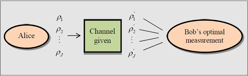
Figure 1: Schematic setup of quantum communication scenario.

Kraus representation of a Quantum Channel: We use a set of Kraus operators $K_{m}(m=1,...,N)$ to represent the quantum channel, such that

$$\sum_{m=1}^{N}K_{m}^{\dagger}K_{m}=1\,.$$ (1)

Consider the following quantum communication scenario shown in Fig. 1. Alice sends a set of quantum states $\mathcal{E}=\{\rho_{j}\mid j=1,2,...,J\}$ with $\rho_{j}\geq 0$ to Bob through a quantum channel $M$, such that

$$\rho=\sum_{j=1}^{J}\rho_{j}\quad\mbox{with}\;\mathrm{tr}\{\rho\}=1\,.$$ (2)

The states after passing through the channel are given by

$$\rho_{j}^{\prime}=\sum_{m=1}^{N}K_{m}\rho_{j}K_{m}^{\dagger}=M\rho_{j}\,.$$ (3)

Bob performs a generalized measurement, specified by a positive-operator-valued measure (POVM), on the state he receives. The POVM with outcomes $\Pi_{k}(k=1,2,...,K)$ decomposes the identity,

$$\sum_{k=1}^{K}\Pi_{k}=1\quad\mbox{with}\;\Pi_{k}\geq 0\,.$$ (4)

Then, the joint probability to receive the jth state and get the kth outcome is

$$p_{jk}=\mathrm{tr}\{\rho_{j}^{\prime}\Pi_{k}\}\,,\quad\sum_{j,k}p_{jk}=1\,.$$ (5)

Bob’s figure of merit is the mutual information

$$I(\mathcal{E};\Pi)=\sum_{j=1}^{J}\sum_{k=1}^{K}p_{jk}\log_{2}\frac{p_{jk}}{p_{j\cdot}p_{\cdot k}}\,.$$ (6)

where $p_{j\cdot}$ and $p_{\cdot k}$ are the marginal probabilities,

$$p_{j\cdot}=\sum_{k}p_{jk}=\mathrm{tr}\{\rho_{j}\}\,,\quad p_{\cdot k}=\sum_{j}p_{jk}=\sum_{m}\mathrm{tr}\{\rho(K_{m}^{\dagger}\Pi_{k}K_{m})\}\,.$$ (7)

As stated, the $\rho_{j}$s are normalized such that their traces equal the probabilities of receiving them.

Classical Capacity of Quantum Channels: Generally, the classical capacity of a quantum channel can be defined as the maximum accessible information with respect to both statistical operators and POVM outcomes,

$$\mathrm{\emph{C}}=\max_{\mathcal{E}}\max_{\Pi}I(\mathcal{E};\Pi)\,.$$ (8)

Given a certain quantum channel, SeCQC finds the statistical operators as well as POVM outcomes that maximize the accessible information (AI), and thus determines the classical capacity of the quantum channel.

The calculation is performed using a combination of the steepest-ascent method (see Ref. [2] and Section 11.5 in Ref. [3]) and the conjugate-gradients (CG) method [4]. The percentage chance to calculate with one method or the other can be specified by the user (see Section 4 below). The implementation in SeCQC also makes use of the golden-section search method.

3 Download and Compile

The complete set of files, including this manual, are available at the SeCQC site: http://www.quantumlah.org/publications/software/SeCQC/. Download http://www.quantumlah.org/publications/software/SeCQC/all.tar.gz, if you want to have the complete collection of files. Just this manual is fetched from http://www.quantumlah.org/publications/software/SeCQC/Manual.pdf. The Windows executable file for SeCQC can be downloaded from http://www.quantumlah.org/publications/software/SeCQC/secqc.tar.gz. If you intend to modify the code, you can download the source files from http://www.quantumlah.org/publications/software/SeCQC/source.tar.gz.

The program is written in C++ and the graphic user interface (GUI) is implemented using wxWidgets (http://www.wxwidgets.org/). Here are the instructions for compiling SeCQC:

1. Install wxWidgets from http://www.wxwidgets.org/downloads/.

2. If you are working in Windows, you need to install MinGW (http://www.mingw.org/download.shtml) and MYSY (http://www.mingw.org/msys.shtml) as well.

3. When wxWidgets and MinGW are configured, you can compile SeCQC by executing g++ MI.cpp ‘wx-config –libs‘ ‘wx-config –cxxflags‘ -o YourProgramName in MSYS shell.

4. If you face problems running the program in a Linux environment, try export LD_LIBRARY_PATH=/usr/local/lib.

5. The executable file is compiled under Windows XP Service Pack 3, with wxWidgets 2.8.10, MinGW 5.1.6 and MSYS 1.0.11.

4 How to use the program

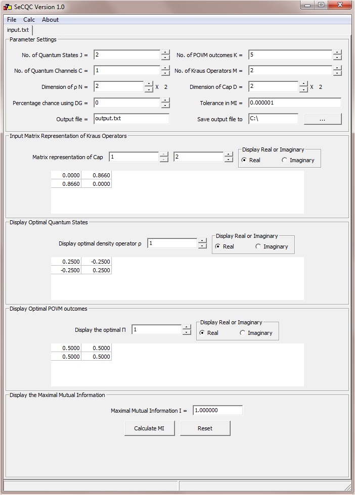
Figure 2: The graphical user interface (GUI) of the program.

The GUI of SeCQC is shown in Fig. 2. In the first box labeled as “Parameter Settings”, $J$ is the number of statistical operators $\rho_{j}$. The current maximum possible value is $J=30$. Parameter $K$ is the initial number of POVM outcomes, with the largest possible value being $K=30$. The third and fourth fields are the number $C$ of Quantum Channels to be inserted and the number $M$ of Kraus operators for each channel respectively. The next two fields are the dimension $D$ of Kraus operators and the dimension $N$ of statistical operators respectively with 30 being their highest possible value. All the maximum values mentioned above can be changed by modifying the source code. The seventh field is the percentage chance to use the steepest-ascent method to perform maximization in an iteration; this parameter controls the relative frequency of using the direct or the conjugate gradient. The eighth field gives the tolerance in the accessible information, the stopping criteria for the computation; the calculation stops when the difference in accessible information between the current iteration and the previous iteration is less than half of the sum multiplied by the tolerance plus the $\mathrm{machine\_epsilon}$ $\epsilon_{m}$ (also termed as the machine accuracy, typical value for double precision is around $1.6\times 10^{-16}$), i.e. when $2.0\times(\mathrm{current}-\mathrm{previous})\leq\mathrm{tolerance}\times(\mathrm{current}+\mathrm{previous})+\epsilon_{m}$. The ninth field is the name of the output file. By default, the output file will be located at hard disk C. You can change the output directory by clicking the ellipsis button “…” and choose your preferred location.

The next three boxes display the input Kraus operators $\{K_{m}\}_{m=1,\dots,M}$, the optimal statistical operators $\{\rho_{j}\}_{j=1,\dots,J}$ and the calculated optimal POVM outcomes $\{\Pi_{k}\}_{k=1,\dots,K}$. The spin buttons are used to switch between the various $K_{m}$s/$\rho_{j}$s/$\Pi_{k}$s, while the small box beside the spin button is used to choose to display the real or imaginary part of the chosen $K_{m}$s/$\rho_{j}$s/$\Pi_{k}$s.

The maximum accessible information for the given channel will be displayed in the last box after the “Calculate MI” button is pressed. All values will be reset to default when the “Reset” button is pressed.

Important note: The matrices for the $K_{m}$s must have the correct dimension; they must satisfy the condition, i.e. $\sum_{m}K_{m}^{\dagger}K_{m}=1$.

5 How to import data

Data can be imported into SeCQC using a text file that is possibly generated by another program. An example is shown in Fig. 3. When importing, the numbers after the equal signs will be read into the program. The first line is the dimension $D$ of the Kraus operators. The second line gives the dimension $N$ of the statistical operators. The third line gives the number $J$ of the statistical operators and the fourth line gives the number of outcomes $K$ of POVMs that the program should start calculating with. And the last two lines give the number $M$ of the Kraus operators for each channel and the number $C$ of Quantum Channels respectively.

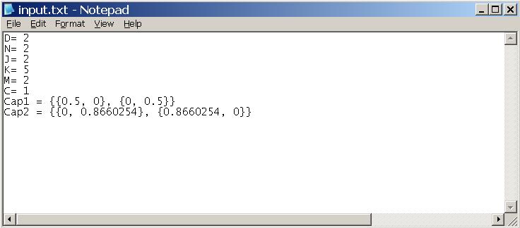
Figure 3: Example of an import file.

The subsequent lines give the input matrices for the Kraus operators. Each line will give only one operator. For an operator represented in matrix form as

$$\left(\begin{array}[]{cc}0.1&0.3+0.5i\\ 0.3-0.5i&0.6\end{array}\right),$$ (9)

the input data should be formatted as $\{\{0.1,0.3+0.5\mathrm{\texttt{I}}\},\{0.3-0.5\mathrm{\texttt{I}},0.6\}\}$.

Complex numbers are entered as $\mathrm{RealPart}+\mathrm{ImaginaryPart}\,\mathrm{\texttt{I}}$, as illustrated by $-3.1-4.5\mathrm{\texttt{I}}$. Please note that the complex unit $i$ must be entered in upper case I and it must be at the end of the entry.

6 Meaning of output data

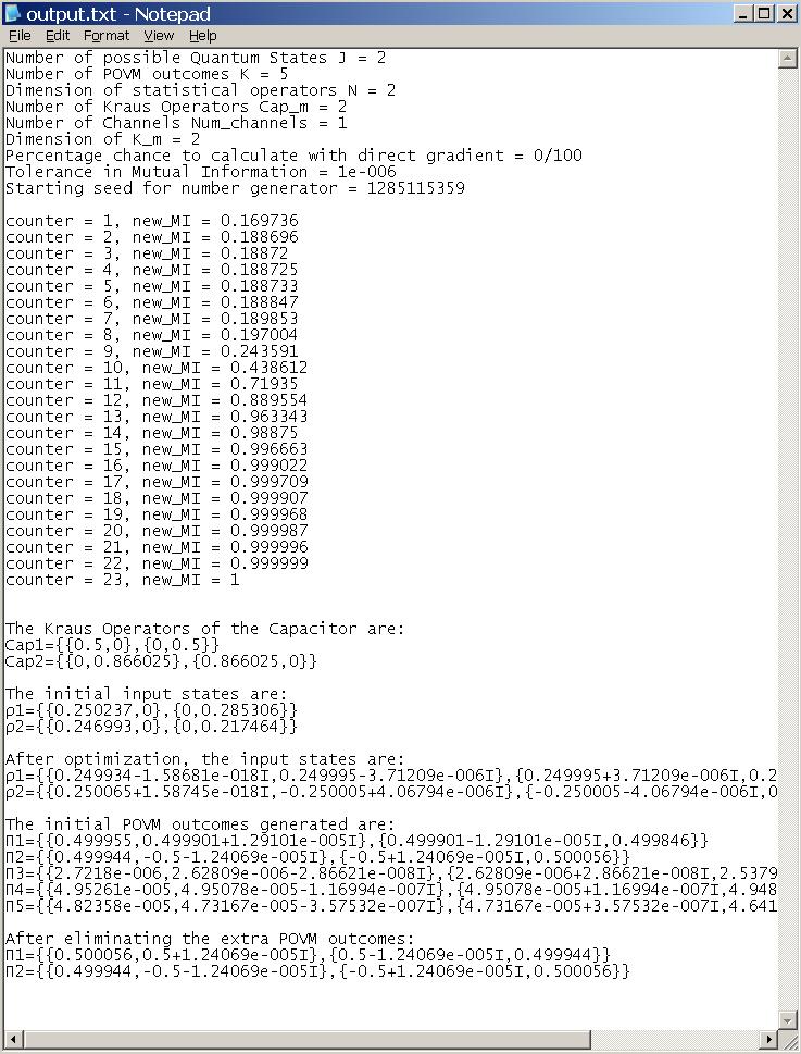
Figure 4: Example of output file.

A typical output file looks like Fig. 4. The first eight lines give the following information: the number $J$ of statistical operators, the initial number $K$ of POVM outcomes, the dimension $N$ of the statistical operators, the number $M$ of Kraus operators for each channel, the number $C$ of Quantum Channels inserted, the dimension $D$ of the Kraus operators, the tolerance in the calculated mutual information, and the seed for the random number generator.

The next block of lines gives the mutual information at the end of each iteration. In the example shown in Fig. 4, altogether 26 iterations have been performed with the final accessible information being $\mathrm{AI}=1.000$ exactly.

The subsequent five blocks of lines give the $M$ Kraus operators for each channel, the initial as well as the optimized $J$ statistical operators and the $K$ outcomes of the optimal POVMs that correspond to the accessible information calculated in the final round of iteration. Each Kraus oeprator/statistical operator/POVM outcome is given in a single line in matrix form, as explained in Section 5.

Among the $K$ outcomes, if any two outcomes, say $\Pi_{k_{1}}$ and $\Pi_{k_{2}}$, give equivalent probabilities, i.e. $p_{jk_{1}}p_{\cdot k_{2}}=p_{\cdot k_{1}}p_{jk_{2}}$ for all $j$, then these two POVM outcomes are replaced with one new POVM outcome, $\Pi_{k_{1}}+\Pi_{k_{2}}$, such that the new optimal POVM contains only $K-1$ outcomes. The last block of data in the output file gives the POVM after this elimination process, i.e. the POVM is the optimal POVM with the least number of outcomes.

Caution: As is the case for all steepest-ascent methods, there is the possibility of convergence towards a local, rather than a global, maximum. There is no absolute protection against this danger, but in practice one can fight it efficiently by running the program many times for comparison, with different seeds. It also helps to start with a rather large $K$ value.

7 Contact information

Please send your comments, suggestions, or bug reports to the following email account: secqc@quantumlah.org

8 Acknowledgments

We acknowledge many valuable discussions with S.Y. Looi. Centre for Quantum Technologies (CQT) is a Research Centre of Excellence funded by Ministry of Education and National Research Foundation of Singapore.

References

- [1] K. L. Lee, J. W. Shang, W. K. Chua, S. Y. Looi, and B.-G. Englert, SOMIM: An open-source program code for the numerical Search for Optimal Measurements by an Iterative Method, arXiv:0805.2847 (http://arxiv.org/abs/0805.2847), SOMIM web site (http://www.quantumlah.org/publications/software/SOMIM/).
- [2] J. Řeháček, B.-G. Englert, and D. Kaszlikowski, Iterative procedure for computing accessible information in quantum communication, Phys. Rev. A 71, 054303 (2005); eprint available at http://arxiv.org/pdf/quant-ph/0408134.
- [3] J. Suzuki, S. M. Assad, and B.-G. Englert, “Accessible information about quantum states: An open optimization problem”, Chapter 11 in Mathematics of Quantum Computation and Quantum Technology, edited by G. Chen, S. J. Lomonaco, and L. Kauffman (Chapman & Hall/CRC, Boca Raton 2007), pp. 309–348; also available at http://physics.nus.edu.sg/~phyebg/Papers/135.pdf.
- [4] W. H. Press, B. P. Flannery, S. A. Teukolsky, W. T. Vetterling, “Minimization or Maximazation of Functions”, Chapter 10 in Numerical Recipes in C: The Art of Scientific Computing, (Cambridge University Press, 2nd edition 1992), pp. 394–455.