STRUCTURE AND DYNAMICS OF POLYNOMIAL DYNAMICAL SYSTEMS

Abstract

Discrete models have a long tradition in engineering, including finite state machines, Boolean networks, Petri nets, and agent-based models. Of particular importance is the question of how the model structure constrains its dynamics. This paper discusses an algebraic framework to study such questions. The systems discussed here are given by mappings on an affine space over a finite field, whose coordinate functions are polynomials. They form a general class of models which can represent many discrete model types. Assigning to such a system its dependency graph, that is, the directed graph that indicates the variable dependencies, provides a mapping from systems to graphs. A basic property of this mapping is derived and used to prove that dynamical systems with an acyclic dependency graph can only have a unique fixed point in their phase space and no periodic orbits. This result is then applied to a published model of in vitro virus competition.

1 Introduction

In several areas of engineering, discrete mathematical models, such as finite state machines, Boolean networks, Petri nets, or agent-based models, play an important role in modeling processes that can be viewed as evolving in discrete time, in which state variables have only finitely many possible states. Decision processes, electrical switching networks, or intra-cellular molecular networks represent examples. There is a long tradition in the engineering literature of work related to an understanding of how the structure of such models constrains their dynamics, see, e.g., [3, 2]. This problem is important both for the design of networks as well as for their analysis. In both theoretical and applied studies of dynamical systems, the problem of predicting dynamic features of the system from structural properties is very important, see, e.g., [7, 9]. An instantiation of this problem is the question in systems biology whether the connectivity structure of molecular networks, such as metabolic or gene regulatory networks, has special features that correlate with the type of dynamics these networks exhibit. (This type of application motivated the present study.) Some progress has been made on this question. For instance, in [1] it was shown that certain small network motifs appear much more often in such networks than would be expected in a random graph. The work in this paper was motivated by the desire to provide a theoretical framework within which the relationship between structure and dynamics of certain families of dynamical systems can be studied. We briefly describe this framework and show one example of a result and its implications.

The type of dynamical system studied here is discrete in time as well as in variable states. That is, we consider a collection $x_{1},\ldots,x_{n}$ of variables, each of which can take on values in a finite set $X$. We consider time-discrete dynamical systems

$$f:X^{n}\longrightarrow X^{n}.$$

A well-known instantiation of such systems are Boolean networks, which have many applications in molecular biology as well as engineering. In this case, $X=\{0,1\}$. As described, such systems are set functions without additional mathematical structure. It is therefore advantageous to impose additional mathematical structure on $X$, namely that of a finite field. This is of course utilized in the case of Boolean networks. Evaluation of Boolean functions is equivalent to carrying out arithmetic in the Boolean field with two elements. The translation between Boolean functions and polynomials is straight-forward, with the Boolean operator AND corresponding to multiplication, addition corresponding to XOR, and negation corresponding to addition of $1$. Once we have a finite field structure on $X$, which we shall now denote by $\mathbb{K}$, it is well-known that any function $\mathbb{K}^{n}\longrightarrow\mathbb{K}$ can be represented as a polynomial function [8, p. 369]. Thus, we can focus on systems

$$f=(f_{1},\ldots,f_{n}):\mathbb{K}^{n}\longrightarrow\mathbb{K}^{n},$$

for which each $f_{i}$ is a polynomial function in the variables $x_{1},\ldots,x_{n}$. We will call such a system a polynomial dynamical system (PDS) over $\mathbb{K}$. A powerful consequence is that one can use algorithms and theoretical results from computer algebra and computational algebraic geometry, such as the theory of Gröbner bases.

It has been shown [10, 5] that discrete models in several different frameworks can be translated into the PDS framework, namely $k$-bounded Petri nets, so-called logical models used in molecular biology, and many agent-based models, which are becoming very prominent in biology. Thus, the framework of PDS provides provides a common theoretical formulation. Using algorithms from polynomial algebra, the software package ADAM (Analysis of Dynamic Algebraic Models) [6] is very efficient in analyzing various features of PDS, including their dynamics. Thus, any theoretical results about PDS apply to all these model types.

In this paper, we are concerned with the family $\mathcal{P}$ of all PDS of a given dimension $n$ over a finite field $\mathbb{K}$. The structural information for a PDS includes a directed graph that indicates the dependency relationships between variables. In the context of a molecular network model, this graph would represent the wiring diagram of the network. Graphs can be represented by their adjacency matrices. The set of $n\times n$ matrices carries an algebraic structure using max and min operations, which has been studied previously over the real field, see, e.g., [4]. Here we prove a result about the relationship between properties of dynamical systems in $\mathcal{P}$ under composition and properties of the corresponding adjacency matrices in the max-min algebra. As a consequence of this result, we derive a dynamic property of PDS with acyclic dependency graphs. Finally, we give an application of this consequence to a published model of in vitro virus competition.

2 The algebra of dynamical systems

Let $\mathbb{K}$ be any finite field. We consider dynamical systems

$$f=(f_{1},\ldots,f_{n}):\mathbb{K}^{n}\rightarrow\mathbb{K}^{n},$$

where $f_{i}:\mathbb{K}^{n}\rightarrow\mathbb{K}$ for $i=1,\ldots,n$. As observed above, any such $f$ is a PDS. Let $\mathcal{P}$ denote the family of all such systems. It is well-known that $\mathcal{P}$ has the structure of an associative algebra under coordinate-wise addition and composition of functions.

To $f$ we can associate a directed graph with the $n$ nodes $x_{1},\ldots,x_{n}$. There is a directed edge from $x_{j}$ to $x_{i}$ if $x_{j}$ appears in $f_{i}$. Let $[f]$ be the $n\times n$ adjacency matrix of this graph. That is, $[f]=(a_{ij})$ is defined as follows:

$$a_{ij}=\left\{\begin{array}[]{ll}1&f_{i}\text{ depends on }x_{j}\\ 0&\text{otherwise}\end{array}\right.$$

Equivalently, $a_{ij}=1$ if and only if there are $p\neq q\in\mathbb{K}$ such that

$$f_{i}(x^{(j,p)})\neq f_{i}(x^{(j,q)})$$

where $x^{(j,p)}=(x_{1},\dots,x_{j-1},p,x_{j+1},\dots,x_{n})\in\mathbb{K}^{n}$.

The adjacency matrix has binary entries, and we now define two operations on such matrices. Let $\mathbb{B}$ denote the Boolean field with two elements, with the natural order $0<1$.

Definition 2.1.

Given $a,b\in\mathbb{B}$, we let:

1)

$a\oplus b=\max\{a,b\}$ and

2)

$a\star b=\min\{a,b\}$

Definition 2.2.

Given $A=(a_{ij})$ and $B=(b_{ij})$ matrices with entries in $\mathbb{B}$, we define the following operation:
$A\star B=C=(c_{ij})$, where $c_{ij}=\bigoplus^{n}_{k=1}(a_{ik}\star b_{kj})$

Remark 2.1.

$c_{ij}=1$ if and only if there is $k$ such that $a_{ik}\star b_{kj}=1$

Definition 2.3.

We define $A\preceq B$ if and only if $a_{ij}\leq b_{ij}$ for all i,j.

Forming the adjacency matrix of the dependency graph of a PDS then gives a mapping

$$\mathcal{P}\longrightarrow\mathcal{M}.$$

And we also have a mapping that associates to an element in $\mathcal{P}$ its phase space, a directed graph on the vertex set $|\mathbb{K}^{n}|$, which encodes the dynamics of the system. We will denote by $\mathcal{S}$ the set of all directed graphs on $|\mathbb{K}^{n}|$ with the property that each vertex has a unique outgoing edge (the requirement for being the phase space of a deterministic PDS). Hence, we have mappings

$$\mathcal{S}\longleftarrow\mathcal{P}\longrightarrow\mathcal{M}.$$

The result in the next section relates information in $\mathcal{M}$ to information in $\mathcal{S}$.

3 A property of $\mathcal{P}\longrightarrow\mathcal{M}$

The main result of this paper is the following theorem. It describes a basic property of the mapping that extracts the adjacency matrix from the system.

Theorem 3.1.

We have that $[f\circ g]\preceq[f]\star[g]$ in $\mathcal{M}$ for all $f,\ g\in\mathcal{P}$.

Proof.

Let $A$, $B$, and $C$ be the adjacency matrices for $f$, $g$, and $f\circ g$, respectively. It suffices to prove that, if $c_{ij}=1$, then $a_{ik}b_{kj}=1$ for some $k$. Let us assume that $c_{ij}=1$, then there are $p\neq q\in\mathbb{K}$ such that

$$(f\circ g)_{i}(x^{(j,p)})\neq(f\circ g)_{i}(x^{(j,q)}),$$

where $x^{(j,p)}=(x_{1},\ldots,x_{j-1},p,x_{j+1},\ldots,x_{n})\in\mathbb{K}^{n}$. Now, since $(f\circ g)_{i}=f_{i}\circ g$ we have that

$$f_{i}(y_{1},\dots,y_{n})\neq f_{i}(\hat{y}_{1},\dots,\hat{y}_{n}),$$

where $y_{s}=g_{s}(x^{(j,p)})$ and $\hat{y}_{s}=g_{s}(x^{(j,q)})$ for $s=1,\dots,n$. Then there is an index $k$ such that $f_{i}$ depends on $x_{k}$ and

$$y_{k}\neq\hat{y}_{k},$$

or

$$g_{k}(x^{(j,p)})\neq g_{k}(x^{(j,q)}).$$

Therefore, $a_{ik}=1$ and $b_{kj}=1$ and, consequently, $a_{ik}b_{kj}=1$. ∎

Corollary 3.2.

$[f^{r}]\preceq[f]^{r}$ for all $f\in\mathcal{P}$, and for any $r\geq 1$.

Proof.

Replace $g$ by $f$ in Theorem 3.1. ∎

4 PDS with acyclic dependency graph

As an easy application of our main result we now consider PDS in $\mathcal{P}$ that have an acyclic dependency graph, that is, no feedback loops in their structure. For any $f:\mathbb{K}^{n}\rightarrow\mathbb{K}^{n}$ with acyclic dependency graph we can see easily that its adjacency matrix $[f]$ is a strictly triangular matrix, i.e., with zeros in the diagonal (otherwise, there would be loops in the graph). Therefore, its characteristic polynomial is equal to $\lambda^{r}$, where $r$ is the order of the matrix. So $[f]$ is nilpotent and $[f]^{r}=0$.

Corollary 4.1.

Any discrete dynamical system $f:\mathbb{K}^{n}\rightarrow\mathbb{K}^{n}$ with acyclic dependency graph has a unique fixed point.

Proof.

By Corollary 3.2, $[f^{r}]\preceq[f]^{r}=0$, so $f^{r}$ is constant: $f^{r}\equiv x_{0}$. Therefore, $x_{0}$ is the unique fixed point of $f$.

∎

Note that the nilpotency index of $[f]$, the smallest integer $r$ for which $[f]^{r}=0$ and $[f]^{r-1}\neq 0$, gives us an upper bound for the number of steps to reach the unique fixed point from any other state.

5 Application

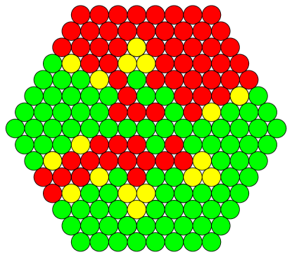
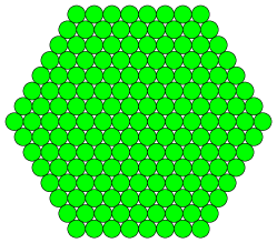
In this section we will present an application of Corollary 4.1 to a published model of an in vitro competition between two strains of a murine coronavirus studied in Jarrah et. al. [11]. The model is presented as a hexagonal grid of cells, with color coding of cells to indicate their infection status. Normal cells are represented as white. Infected cells are represented as red or green, or yellow, in the case of dual infection. The infection spreads from the center outwards. At each time step one ring of new cells is infected. The outcome of a cell in the new ring depends on the infection status of its two neighbors in the previous infected ring. The local update function for each cell is constructed using the following rules:

• If a cell has only one infected neighbor, it will get the same type of infection.

• If a cell has two infected neighbors, then we use the following table to determine the type of infection of that cell.

Rules for the update function
	Green	White	Red	Yellow
Green	Green	Green	Yellow	Green
White	Green	White	Red	Yellow
Red	Yellow	Red	Red	Red
Yellow	Green	Yellow	Red	Yellow

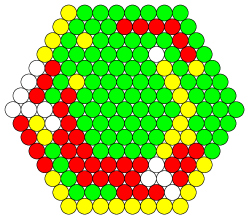
The dynamics of this system is represented in Figure 1. In this example we will use 169 cells. In order to simulate experimental conditions described in [11] we initialize the infection using the 37 center cells. Each cell can have only one of four colors at a time. We use the field with four elements, $\mathbb{F}_{4}=\{0,1,2,3\}$, to represent the set of different colors. The color assignment is as follows.

Color assignment
Color	Field element
Green	0
Red	1
White	2
Yellow	3

We represent the 169 cells by the variables $x_{1},\dots,x_{169}$, with $x_{1},\dots,x_{37}$ representing the center cells. The variables $x_{128},\dots,x_{169}$ represents the cells in the outermost ring.

In [11] the system was studied from the point of view of the experimental system. There, a collection of cells was infected in the center of the dish, and the infection was then observed to spread to the rest of the Petri dish in a pattern that showed distinct segmentation, matching the experimental results. In order to mimic the biological system, it was assumed that the cells initially infected did not change their infection state subsequently, so that the model is constrained and heterogeneous with respect to the rules assigned to all the nodes. This, in effect, changes the dynamical system since those cells are now assigned constant functions rather than the rules described above. The outcome is a steady state that shows a characteristic segmentation which coincides with experimental observations. See Figure 1 for an example.

Figure 1: Dynamics of the constrained model

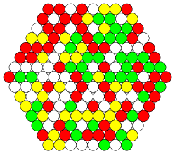
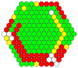
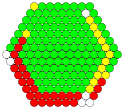
If, however, we allow all cells to evolve according to the update rule above, then the outcome is significantly different. In that case, the center cell plays a very special role. It is represented by the only node in the network that does not receive any inputs from other cells and is therefore constant. (Note that, in order to have an acyclic dependency graph, a PDS must have at least one node without incoming edges.) The state of that node then plays the role of an external parameter, and a particular choice of state/color for this node is part of the system description. In this case Corollary 4.1 applies, since the dependency graph of the network is acyclic. See Figure 2.

Figure 2: Adjacency graph for virus competition

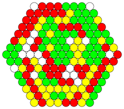
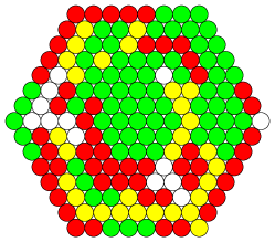
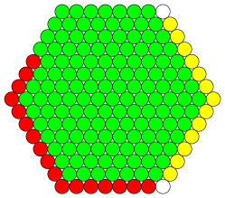
We conclude that in this case any initialization of the system, that is, any assignment of colors to each of the nodes in the network, results in a unique steady state, namely the state in which all nodes have the same color as the center node. In effect, what happens is that after initializing the 37 nodes in the center they propagate a distinct, segmentation-like pattern. At the same time, the color in the center cell propagates outward and overpowers the segmentation pattern, resulting in a system state with a homogenous color distribution. See Figure 3.

If we now assume that a larger number of cells in the center is infected, that is, is assigned a color that does not change subsequently, as in the initial experiments, then the color distribution along the edge of the infected region propagates and produces a steady state that show the segmentation patterns observed in [11].

The polynomial dynamical system for the model in which all cells are allowed to change is represented as

$$f=(f_{1},\dots,f_{169}):\mathbb{F}_{4}^{169}\rightarrow\mathbb{F}_{4}^{169}$$

The coordinate functions $f_{i}$ are polynomials in $\mathbb{F}_{4}[x_{j},x_{k}]$, where $x_{j}$ and $x_{k}$ are the two neighbors of $x_{i}$ in the previous infected ring. Let $x_{i}$ represent one of the 169 cells, then $x_{i}$ is updated according $f_{i}(x_{j},x_{k})$, i.e. $x_{i}=f_{i}(x_{j},x_{k})$, where $x_{j}$ and $x_{k}$ are the two neighbors of $x_{i}$ in the previous infected ring. The following table specifies part of the truth table for $f_{i}(x_{j},x_{k})$,

Truth Table
Color	Color	$x_{j}$	$x_{k}$	$f(x_{j},x_{k})$	Color
Green	Green	0	0	0	Green
Green	Red	0	1	3	Yellow
Green	White	0	2	0	Green
Green	Yellow	0	3	0	Green
Red	Green	1	0	3	Yellow
Red	Red	1	1	1	Red
Red	White	1	2	1	Red
Red	Yellow	1	3	1	Red

Written as a polynomial, $f_{i}$ has the following form

$$\begin{array}[]{lcl}f_{i}(x_{j},x_{k})&=&x_{j}+3x_{j}^{2}+x_{j}^{3}+3x_{j}^{4}+x_{k}+3x_{j}x_{k}+\\ \\ &&x_{j}^{2}x_{k}+x_{j}^{3}x_{k}+2x_{j}^{4}x_{k}+3x_{k}^{2}+x_{j}x_{k}^{2}+\\ \\ &&4x_{j}^{2}x_{k}^{2}+4x_{j}^{4}x_{k}^{2}+x_{k}^{3}+4x_{j}^{2}x_{k}^{4}+\\ \\ &&3x_{j}^{3}x_{k}^{4}+3x_{j}^{4}x_{k}^{4}\end{array}$$

This polynomial form can then be used to compute the steady state configuration by solving a system of polynomial equations.

Figure 3: Dynamics where all cells evolve according to the rules. The center cell determines the final outcome.

6 ODEs with acyclic dependency graph

As an aside note we will mention that our main result is also valid for dynamical systems with differential equations. We now consider ODEs that have an acyclic dependency graph, that is, no feedback loops in their structure. For any ODE with acyclic dependency graph we can see easily that its adjacency matrix $[f]$ is a strictly triangular matrix, i.e., with zeros in the diagonal (otherwise, there would be loops in the graph).

Theorem 6.1.

Consider an ODE with acyclic dependency graph, then there is a unique steady state and it is asymptotically stable.

To proof this we need the following lemma.

Lemma 6.2.

Let $z:[0,\infty)\rightarrow\mathbb{R}$ be a continuous function such that $\lim_{t\rightarrow\infty}z(t)=z_{0}\in\mathbb{R}$. If $y^{\prime}=z-ky,y(0)=y_{0}$ with $k>0$, then $\lim_{t\rightarrow\infty}y(t)=\frac{z_{0}}{k}$ (regardless of the value of $y_{0}$).

Proof.

First, notice that from $y^{\prime}=z-ky$ we obtain $y(t)=y_{0}e^{-kt}+\int_{0}^{t}{e^{k(s-t)}z(s)ds}$. Furthermore, $y(t)-\frac{z_{0}}{k}=y_{0}e^{-kt}+\int_{0}^{t}{e^{k(s-t)}(z(s)-z_{0})ds}+\int_{0}^{t}{e^{k(s-t)}z_{0}ds}-\frac{z_{0}}{k}$. It is easy to show that $\lim_{t\rightarrow\infty}\int_{0}^{t}{e^{k(s-t)}z_{0}ds}-\frac{z_{0}}{k}=\lim_{t\rightarrow\infty}y_{0}e^{-kt}=0$; then, we only need to show that $\lim_{t\rightarrow\infty}\int_{0}^{t}{e^{k(s-t)}(z(s)-z_{0})ds}=0$. First, since $\lim_{t\rightarrow\infty}z(t)=z_{0}$, it follows that $z(s)$ is bounded (let us say by $M$) and $\lim_{t\rightarrow\infty}sup_{s\in[\frac{t}{2},t]}\{|z(s)-z_{0}|\}=0$. On the other hand we have

$|\int_{0}^{t}{e^{k(s-t)}(z(s)-z_{0})ds}|\leq$

$\int_{0}^{\frac{t}{2}}e^{k(s-t)}|z(s)-z_{0}|ds+\int_{\frac{t}{2}}^{t}e^{k(s-t)}|z(s)-z_{0}|ds$

$\leq 2M\int_{0}^{\frac{t}{2}}e^{k(s-t)}ds+$

$sup_{s\in[\frac{t}{2},t]}\{|z(s)-z_{0}|\}\int_{\frac{t}{2}}^{t}e^{k(s-t)}ds$

$=2M\frac{e^{-kt/2}-e^{-kt}}{k}+$

$\ \ \ sup_{s\in[\frac{t}{2},t]}\{|z(s)-z_{0}|\}\frac{1-e^{-kt/2}}{k}$

$\leq 2M\frac{e^{-kt/2}}{k}+sup_{s\in[\frac{t}{2},t]}\{|z(s)-z_{0}|\}\frac{1}{k}$

The last expression converges to 0 as $t\rightarrow\infty$ and this finishes the proof.

∎

Corollary 6.3.

Consider $x:[0,\infty)\rightarrow\mathbb{R}^{n}$, $f:\mathbb{R}^{n}\rightarrow\mathbb{R}$ continuous such that $\lim_{t\rightarrow\infty}x(t)=x_{0}\in\mathbb{R}^{n}$. If $y^{\prime}=f(x)-ky$ with $k>0$, then $\lim_{t\rightarrow\infty}y(t)=\frac{f(x_{0})}{k}$.

Proof.

It is enough to consider $z(t)=f(x(t))$ and apply the lemma above. ∎

When modeling biological systems using ODEs, it is common for the functions to have natural decay; that is, they are of the form $x_{i}^{\prime}=f(x)-k_{i}x_{i}$ for $i=1,\ldots,n$. The dependency graph of such an ODE is the graph with nodes $\{1,\ldots,n\}$ and an edge from $i$ to $j$ if $f_{j}$ depends on $x_{i}$.

Proof of theorem 6.1.

Consider an ODE with natural decay. Without loss of generality, we consider that the adjacency matrix of the dependency graph is of the form

$$\left[\begin{array}[]{ccccc}0&0&0&\ldots&0\\ &0&0&\ldots&0\\ &*&0&\ldots&0\\ \vdots&&&\ddots&\\ &*&\ldots&*&0\end{array}\right]$$

That is, $f_{i}=f_{i}(x_{1},\ldots,x_{i-1})$ ($f_{i}$ could depend on less variables). For $i=1$ we have $x_{1}^{\prime}=f_{1}-k_{1}x_{1}$ where $f_{1}$ is constant. Then, $\lim_{t\rightarrow\infty}x_{1}(t)=s_{1}$, where $s_{1}=\frac{f_{1}}{k_{1}}$. For $i=2$ we have $x_{2}^{\prime}=f_{2}(x_{1})-k_{2}x_{2}$; then, by the corollary, we have that $\lim_{t\rightarrow\infty}x_{2}(t)=s_{2}$, where $s_{2}=\frac{f_{2}(s_{1})}{k_{2}}$. By induction, if $\lim_{t\rightarrow\infty}(x_{1}(t),\ldots,x_{i-1}(t))=(s_{1},\ldots,s_{i-1})$ and $x_{i}^{\prime}=f_{i}(x_{1},\ldots,x_{i-1})-k_{i}x_{i}$, then $\lim_{t\rightarrow\infty}x_{i}(t)=s_{i}$, where $s_{i}=\frac{f_{i}(s_{1},\ldots,s_{i-1})}{k_{i}}$. At the end, we have $s=(s_{1},\ldots,s_{n})\in\mathbb{R}^{n}$ such that $\lim_{t\rightarrow\infty}x(t)=s$ (regardless of the value of $x(0)$). It follows that $s$ is the unique steady state and that it is asymptotically stable. ∎

7 Discussion

In this paper we have shown that it is fruitful to study the relationship between the structure and the dynamics of discrete dynamical systems by looking at the algebraic properties of the mapping $\mathcal{P}\longrightarrow\mathcal{M}$ from the algebra of PDS to the algebra of adjacency matrices. With a very straightforward proof we have shown that dynamics is very simple in the absence of feedback loops. It is worth observing that this result, Corollary 4.1, could also have been obtained as a consequence of a more general result that says that for the existence of more than one fixed point, a positive feedback loop is required in the dependency graph, and for periodic orbits to exist a negative feedback is necessary (but not sufficient). This result implies that in order to obtain more than one fixed point or periodic orbits, it is necessary that the dependency graph of the system have feedback loops [9]. However, the proof we have given here of this same result is very simple and stems from a basic property of the mapping $\mathcal{P}\longrightarrow\mathcal{M}$ rather than complicated phase space arguments. It emphasizes our belief that the proper framework for studying the relationship between structure and dynamics of PDS is the algebra inherent in this mapping.

Furthermore, we have shown that one can use Corollary 4.1 to draw non-obvious conclusions about a system of interest. This conclusion would be very difficult to arrive at through simulations, due to the combinatorial complexity of the dynamics on a large grid.

References

- [1] U. Alon (2006) An introduction to systems biology: design principles of biological circuits. Chapman&Hall.
- [2] J. T. Butler, T. Sasao, and M. Matsuura (2005), Average path length of binary decision diagrams. IEEE Trans. Comp. 27: 1041–1053.
- [3] B. Elspas (1959) The theory of autonomous linear sequential networks. IRE Trans. Circuit Theory 6: 45–60.
- [4] M. Gavalec (2001) Monotone eigenspace structure in max-min algebra. Linear Algebra and its Applications 345: 149–167.
- [5] Hinkelmann, F., Murrugarra, D., Jarrah, A.S., and Laubenbacher, R. (2010) A mathematical framework for agent-based models of complex biological networks. Bull. Math. Biol., in press.
- [6] F. Hinkelmann, M. Brandon, B. Guang, R. Mcneill, G. Blekherman, A. Veliz-Cuba, and R. Laubenbacher (2010) ADAM: Analysis of discrete models of biological systems using computer algebra. Under review.
- [7] M. Golubitsky and I. Stewart (2002) Patterns of oscillation in coupled cell systems. Geometry, Mechanics, and Dynamics, 243–286, Springer Verlag, New York.
- [8] R. Lidl and H. Niederreiter (1997) Finite Fields. Encyclopedia of Mathematics and its Applications 20, 2nd ed.. Cambridge University Press, Cambridge.
- [9] C. Soulé (2003) Graphic requirements for multistationarity. ComPlexUs 1: 123–133.
- [10] A. Veliz-Cuba, et al. (2010) Polynomial algebra of discrete models in systems biology. Bioinformatics 26:1637-1643.
- [11] A. Jarrah, et al. An optimal Control Problem For in vitro Virus Competition. 43rd IEEE Conference on Decision and Control, Bahamas, 2004.