Particle Kalman Filtering: A Nonlinear Bayesian Framework for Ensemble Kalman Filters
Abstract
This paper investigates an approximation scheme of the optimal nonlinear Bayesian filter based on the Gaussian mixture representation of the state probability distribution function. The resulting filter is similar to the particle filter, but is different from it in that, the standard weight-type correction in the particle filter is complemented by the Kalman-type correction with the associated covariance matrices in the Gaussian mixture. We show that this filter is an algorithm in between the Kalman filter and the particle filter, and therefore is referred to as the particle Kalman filter (PKF).
In the PKF, the solution of a nonlinear filtering problem is expressed as the weighted average of an “ensemble of Kalman filters” operating in parallel. Running an ensemble of Kalman filters is, however, computationally prohibitive for realistic atmospheric and oceanic data assimilation problems. For this reason, we consider the construction of the PKF through an “ensemble” of ensemble Kalman filters (EnKFs) instead, and call the implementation the particle EnKF (PEnKF). We show that different types of the EnKFs can be considered as special cases of the PEnKF. Similar to the situation in the particle filter, we also introduce a re-sampling step to the PEnKF in order to reduce the risk of weights collapse and improve the performance of the filter. Numerical experiments with the strongly nonlinear Lorenz- model are presented and discussed.
1 Introduction
Estimating the state of the atmosphere and the ocean has long been one of the main goals of modern science. Data assimilation, which consists of combining data and dynamical models to determine the best possible estimate of the state of a system, is now recognized as the best approach to tackle this problem (Ghil and Malanotte-Rizzoli, 1991). The strongly nonlinear character of the atmospheric and oceanic models, combined with their important computational burden, makes data assimilation in these systems quite challenging.
Based on the Bayesian estimation theory, the optimal solution of the nonlinear data assimilation problem can be obtained from the optimal nonlinear filter (ONF) (Doucet et al., 2001). This involves the estimation of the conditional probability distribution function (pdf) (not necessarily Gaussian) of the system state given all available measurements up to the estimation time. Knowledge of the state pdf allows determining different estimates of the state, such as the minimum variance estimate or the maximum a posteriori estimate (Todling, 1999). The ONF recursively operates as a succession of a correction (or analysis) step at measurement times to correct the state (predictive) pdf using the Bayes’ rule, and a prediction step to propagate the state (analysis) pdf to the time of the next available observation. Although conceptually simple, the numerical implementation of the optimal nonlinear filter can be computationally prohibitive, even for systems with few dimensions (Doucet et al., 2001). Its use with atmospheric and oceanic data assimilation problems is therefore not possible because of the huge dimension of these systems.
In recent years, two approximation schemes of the ONF have attracted the attention of researchers for their potentials to tackle nonlinear and non-Gaussian data assimilation problems. One is based on the point-mass representation (mixture of Dirac functions) of the state pdf, and leads to the celebrated particle filter (PF) (Doucet et al., 2001; Pham, 2001; Nakano et al., 2007; Van Leeuwen, 2003, 2009). The other is based on the Gaussian mixture representation of the state pdf, and results in a filter that is in between the Kalman filter and the particle filter (Anderson and Anderson, 1999; Bengtsson et al., 2003; Chen and Liu, 2000; Hoteit et al., 2008; Luo et al., 2010; Sorenson and Alspach, 1971), as to be shown later. For this reason, we refer to this filter as the particle Kalman filter (PKF).
In terms of computational efficiency, the particle filter needs to generate large samples for a good approximation of the state pdf. In certain circumstances, in order to avoid weights collapse, the number of samples needs to scale exponentially with the dimension of the system in assimilation (Bengtsson et al., 2008), which may be infeasible for high-dimensional systems (Snyder et al., 2008). On the other hand, in some comparison studies (Han and Li, 2008; Nakano et al., 2007), it has been reported that the ensemble Kalman filter (EnKF) and its variants (Anderson, 2001; Bishop et al., 2001; Burgers et al., 1998; Evensen, 1994; Evensen and van Leeuwen, 1996; Houtekamer and Mitchell, 1998; Whitaker and Hamill, 2002) can achieve lower estimation errors than the particle filter given a small ensemble size. To save space, in this paper we confine ourselves to the PKF, and make performance comparison only between the PKF and the EnKF.
Using a Gaussian mixture representation of the state pdf, the resulting PKF consists of an ensemble of parallel nonlinear Kalman filters (Hoteit et al., 2008; Luo et al., 2010). Different variants of the Kalman filter (KF), including the extended Kalman filter (Chen and Liu, 2000; Sorenson and Alspach, 1971), the reduced-rank Kalman filter (Hoteit et al., 2008; Luo et al., 2010), the EnKF (Anderson and Anderson, 1999; Bengtsson et al., 2003), can be used to construct the PKF. The focus of this paper is to investigate the PKF that is constructed by an ensemble of parallel EnKFs. Common to all the implementations of the PKF, the mixture of normal distributions (MON) – a more general pdf representation than the single Gaussian pdf approximation in the EnKF – can be used to tackle nonlinearity and non-Gaussianity in data assimilation. On the other hand, choosing the EnKF to construct the PKF is based on the consideration of computational efficiency, since the EnKF itself is a very efficient algorithm for data assimilation in high dimensional systems. In this regard, this work is very similar to the earlier works of Anderson and Anderson (1999) and Bengtsson et al. (2003), but is different from them mainly in the following aspect.
In Anderson and Anderson (1999) and Bengtsson et al. (2003), the PKF was constructed without a re-sampling step. As a result, the PKF may suffer from weights collapse as in the particle filter. To overcome this problem, Bengtsson et al. (2003) considered a hybrid of the EnKF and the PKF, which, however, involves the computation of the inverses of sample covariance matrices in the “global-to-local” adjustments. In doing so, it is not only computationally intensive, but also encounters singularities in computing the inverses when the ensemble size is smaller than the system dimension, such that the sample covariances themselves are rank deficient. Therefore, it is not clear how the hybrid scheme in Bengtsson et al. (2003) can be applied to the scenario with the ensemble size smaller than the system dimension. For the implementation of the PKF scheme in this work, we introduce a re-sampling step similar to those in Musso et al. (2001) and Stavropoulos and Titterington (2001) to tackle weights collapse. Our experience shows that, with this re-sampling step, the PKF becomes much more stable and can conduct data assimilation in the small ensemble scenario, as to be demonstrated through the numerical experiments presented in this work.
As may be of particular interest for the ensemble filtering community, we will show that different EnKFs can be considered as special cases of the PEnKF following our implementation. This point of view allows for a better understanding of the EnKFs’ behaviors and/or their differences.
The paper is organized as follows. The optimal nonlinear filter is first described in section 2. The PKF and its ensemble implementation are discussed in section 3. Results of numerical experiments with the Lorenz- model are presented in section 4. A summary of the main results and a general discussion on the potential of the PEnKF for tackling realistic atmospheric and oceanic data assimilation problems concludes the paper in section 5.
2 The Optimal Nonlinear Filter
Starting from a random initial condition with a known probability density function, the optimal nonlinear filter provides the conditional density function of the system state given all available measurements up to the estimation time. To describe the algorithm of the optimal nonlinear filter, consider the nonlinear stochastic discrete-time dynamical system
| (1) | |||||
| (2) |
where is the state vector (to be estimated), of dimension , is the observation vector, of dimension , and are two continuously differentiable maps from to and from to respectively representing the transition and the observational operators, and and denote the dynamical and the observational noise, respectively. We assume that and are Gaussian with zero mean and non-singular covariance matrices and , respectively, and are independent of the system state at any time instant. Under this setting, the dynamical system Eq. (1) is Markovian.
The optimal nonlinear filter recursively operates with a succession of prediction and correction steps as summarized below. The reader is referred to Doucet et al. (2001) for an extensive description of the filter. To simplify the notation, is defined as a shorthand for the set of all observations up to and including time . Let be the conditional (predictive) pdf of given and be the conditional (analysis) pdf of given , both determined at time . The filter steps are described as follows.
-
Prediction step: Given the analysis pdf at time , the predictive pdf is obtained by integrating with the model (1) to the time of the next available observation . Under the assumptions made on the model noise , the likelihood function for the state vector to transit to at the next time instant is described by the Gaussian pdf , where denotes the Gaussian pdf with mean and covariance . Thus,
(3) -
Correction step: After a new observation has been made, the analysis pdf at time is updated from using Bayes’ rule, i.e.,
(4) The analysis pdf is therefore obtained by multiplying the predictive pdf by the observation likelihood function , and then being normalized by .
While the expressions of the state pdfs can be obtained conceptually, determining the exact values of them at each point of the state space is practically infeasible in high dimensional systems (Doucet et al., 2001). For instance, the determination of the predictive pdf requires the evaluation of the model for a prohibitively large number of , given that one single evaluation might already be computationally very expensive in realistic atmospheric and oceanic applications.
3 The Particle Ensemble Kalman Filter
3.1 Particle Kalman Filtering and Its Ensemble Implementation
Given independent samples from a (multivariate) density , an estimator of can be obtained by the kernel density estimation method (Silverman, 1986), in the form of a mixture of Gaussian pdfs:
| (5) |
where is a positive definite matrix. Inspired from this estimator, the particle Kalman filter (PKF) approximates the conditional state pdfs in the optimal nonlinear filter by mixtures of Gaussian densities of the form
| (6) |
The subscript replaces at the analysis time and at the prediction time. The parameters of the mixture are the weights , the centers of the distributions , and the covariance matrices . In particular, if , reduces to a single Gaussian pdf, so that the PKF reduces to the Kalman filter (KF) or its variants trivially (a non-trivial simplification will also be discussed below). Consequently, the KF and its variants can be considered special cases of the PKF.
Two special cases of Eq. (6) may be of particular interest. In the first case, , such that the Gaussian pdfs tend to a set of Dirac functions , with the mass points at . In this case, the Gaussian mixture Eq. (6) reduces to the Monte Carlo approximation used in the particle filter (Doucet et al., 2001). In the second case, all Gaussian pdfs have (almost) identical centers and covariances, such that the Gaussian mixture Eq. (6) tends to a (single) Gaussian approximation, an assumption often used in various nonlinear Kalman filters (including the EnKF). In this sense, the PKF can be considered as a filter in between the Kalman filter and the particle filter (Hoteit et al., 2008; Luo et al., 2010).
The main procedures of the PKF are summarized as follows. Without loss of generality, suppose that at time instant , the analysis pdf, after a re-sampling step, is given by . Then by applying Eq. (3) at the prediction step, one obtains the background pdf, in terms of a new MON
| (7) |
where and are the propagations of the mean and the covariance of the Gaussian component through the system model Eq. (1), respectively.
Given an incoming observation , one applies Eq. (4) to update to the analysis pdf, also in the form of an MON
| (8) |
where and are updated from and through the Kalman filter or its variants, and the new weights
| (9) |
where is the innovation matrix. If evaluated through the extended Kalman filter, , with being the gradient of evaluated at . Alternatively, if evaluated in the context of the EnKF, can be expressed as the covariance of the projected background ensemble onto the observation space plus the observation covariance (Evensen, 1994; Whitaker and Hamill, 2002). Finally, a re-sampling step can be introduced to improve the performance of the PKF (Hoteit et al., 2008; Luo et al., 2010), so that the analysis pdf becomes . Such a re-sampling algorithm is presented in the next section.
The PKF correction step can be interpreted as composed of two types of corrections: a Kalman-type correction used to update and to and , and a particle-type correction used to update the weights to . In the PKF, the Kalman correction reduces the risk of weights collapse by allocating the estimates (whose projections onto the observation space) far away from the observation relatively more weights than in the particle filter (Hoteit et al., 2008; Van Leeuwen, 2009). Indeed, Eq. (9) has the same form as in the PF (Doucet et al., 2001), but uses the innovation matrices to normalize the model-data misfit, rather than . As are always greater than , the estimates that are close to the observation will receive relatively less weights than in the PF, while those far from the observation will receive relatively more weights. This means that the support of the local predictive pdf and the observation likelihood function will be more coherent than in the PF. Re-sampling will therefore be needed less often, so that Monte Carlo fluctuations are reduced.
The main issue with the PKF is the prohibitive computational burden associated with running an ensemble of KFs, knowing that running a Kalman filter (KF) or an extended KF in high dimensional systems is already a challenge. To reduce computational cost, we use an ensemble of EnKFs, rather than the KF or the extended KF, to construct the PKF. We refer to this approach as the Particle Ensemble Kalman Filter (PEnKF). In the PEnKF, the (analysis) ensembles representing the Gaussian components are propagated forward in time to obtain a set of background ensembles at the next assimilation cycle. Then for each background ensemble, a stochastic or deterministic EnKF is used to update the background ensemble to its analysis counterpart. This amounts to simultaneously running a weighted ensemble of EnKFs, and the final state estimate is the weighted average of all the EnKFs solutions.
3.2 A Re-sampling Algorithm
We adopt a re-sampling algorithm that combines those in Hoteit et al. (2008); Luo et al. (2010); Pham (2001). The main idea is as follows: Given a MON, we first employ an information-theoretic criterion used in Hoteit et al. (2008) and Pham (2001) to check if it needs to conduct re-sampling. If there is such a need, we then re-approximate the MON by a new MON, based on the criterion that the mean and covariance of the new MON match those of the original MON as far as possible Luo et al. (2010).
More concretely, let be the pdf of the -dimensional random vector , expressed in terms of an MON with Gaussian pdfs so that
| (10) |
where are the set of normalized weights of the Gaussian pdfs with mean and covariance , satisfying for and . To decide whether to conduct re-sampling or not, the entropy of the weights is computed, which reads (Hoteit et al., 2008; Pham, 2001)
| (11) |
Ideally, when the distribution of the weights is uniform, which yields the maximum weight entropy , there is no need to conduct re-sampling. Thus, as a criterion, if is within a certain distance to , i.e.,
| (12) |
where is a user-defined threshold, then we choose not to conduct re-sampling. In this work we set the threshold following Hoteit et al. (2008).
In case that there is a need to conduct re-sampling, we follow the procedure similar to that in Luo et al. (2010). Here the idea is to treat re-sampling as a pdf approximation problem, in which we seek a new MON
| (13) |
with equally weighted Gaussian pdfs, to approximate the original in Eq. (10). In approximation, we require that the mean and covariance of be as close as possible to those of . To this end, we need to choose proper values of and in order to achieve this objective.
The means and covariances of and , denoted by and , and and , respectively, are given by
| (14a) | ||||
| (14b) | ||||
Thus our objective is equivalent to balancing the above equation such that
| (15) |
In the trivial case with , Eq. (15) can be satisfied by letting and , and the PEnKF reduces to an EnKF. In non-trivial cases, for simplicity in solving Eq. (15) and reducing computational cost (as to be shown later), one may choose the covariances to be constant, say , for , so that
| (16) |
When an EnKF is used to construct the PKF, one needs to represent the solution of Eq. (16) in terms of some ensembles , where is a matrix containing the (analysis) ensemble of the th Gaussian component in Eq. (13), with mean and covariance . For simplicity, we assume that are all of dimension , with the ensemble size for each . Similar results can be easily obtained in the case with non-uniform ensemble sizes.
We then define a constant , called fraction coefficient hereafter, which satisfies that . We let , so that Eq. (16) is reduced to
| (17) |
In other words, the centers can be generated as a set of state vectors whose sample mean and covariance are and , respectively. After obtaining , one can generate the corresponding ensembles , with the sample means and covariances being and , respectively. How and can be generated is discussed with more details in the support material.
From the above discussion, we see that is a coefficient that decides how to divide among and , so that the constraints in Eq. (16) are satisfied. When , we have so that in Eq. (13) approaches the Monte Carlo approximation in the particle filter, with the mass points equal to . On the other hand, when , we have , so that all approach and approaches . As a result, in Eq. (13) approaches the Gaussian pdf , which is essentially the assumption used in the EnKF. In this sense, when equipped with the re-sampling algorithm, the PEnKF is a filter in between the particle filter and the EnKF, with an adjustable parameter that influences its behavior.
We note that, when , under the constraint of matching the first two moments, our re-sampling scheme is very close to the posterior Gaussian re-sampling strategy used in the Gaussian particle filter (Kotecha and Djurić, 2003; Xiong et al., 2006), in which one generates particles from a Gaussian distribution with mean and covariance equal to those of the posterior pdf of the system states. As a result, there is no guarantee that higher order moments of the new MON match those of the original MON in our re-sampling scheme. If matching higher-order moments is a concern, one may adopt alternative criteria, for instance, the one that aims to minimize the distance (in certain metric) between the new MON and the original one, so that the re-sampling procedure is recast as an optimization problem, in which one aims to choose appropriate parameters, i.e., means and covariances of the new MON, that satisfy the chosen criterion as far as possible. In principle, this type of parameter estimation problem may be solved by the expectation-maximization (EM) algorithm (Redner and Walker, 1984; Smith, 2007). But in practice, it is often computationally very intensive in doing so, due to the slow convergence rate of the EM algorithm and the high dimensionality of the parameter space in constructing the new MON. Therefore we do not consider this type of more sophisticated re-sampling strategy in this study.
For the purpose of pdf re-approximation, it is clear that the MON is not the only choice. A few alternatives are developed in the context of kernel density estimation (KDE) (Silverman, 1986), and in principle all of them can be applied for pdf re-approximation. For instance, KDE is adopted at the re-sampling step in the regularized particle filter (RPF) (Musso et al., 2001; Stavropoulos and Titterington, 2001) to construct a continuous pdf with respect the particles before re-sampling, and to draw a number of new particles from the continuous pdf afterwards. In this regard, the PEnKF is similar to the RPF, especially if the Gaussian kernel is adopted in the RPF for density estimation. However, there also exist differences. We list some of them as follows.
-
•
The RPF first constructs a continuous pdf, and then draws a number of new particles with equal weights from the resulting pdf. In contrast, the PEnKF aims to directly approximate a MON by a new MON with equal weights.
-
•
In the RPF, various kernels can be adopted for the purpose of constructing the continuous pdf. However, in the PEnKF, we are confined to use the MON, since we aim to build the PEnKF consisting of a set of parallel EnKFs.
-
•
The pdf re-approximation criterion used in the PEnKF only captures the first two moments of the underlying pdf. In contrast, KDE used in the RPF in principle can yield a very good pdf estimate, provided that there are sufficient particles. In certain circumstances, though, the number of required particles may also suffer from the “curse-of-dimensionality” (Silverman, 1986, ch. 4).
3.3 Outline of the PEnKF Algorithm
To facilitate the comprehension of the PEnKF, here we provide an outline of the main steps of its algorithm. To avoid distraction, we will discuss the initialization of the PEnKF in the next section. Throughout this paper, we assume that the number of Gaussian components at the re-sampling step and the number of Gaussian components at the prediction and correction steps are time invariant. This implies the choice .
Without loss of generality, we also assume that at time instant , the posterior pdf is re-approximated, through the re-sampling step, by a mixture model
Moreover, the re-approximated analysis ensembles representing the Gaussian components are also generated. The procedures at the next assimilation cycle are outlined as follows.
-
Prediction step: For , propagate the ensembles forward through Eq. (1) to obtain the corresponding background ensembles at instant . Accordingly, the background pdf becomes
with and being the sample mean and covariance of the ensemble , respectively.
-
Correction step: With an incoming observation , for each background ensemble , , apply an EnKF to obtain the analysis mean and the analysis ensemble . During the correction, covariance inflation and localization (cf. § 4.2.2) can be conducted on the EnKF. In addition, update the associated weights to according to Eq (9). After the corrections, the analysis pdf becomes
where are computed according to Eq. (9) in the context of the EnKF, and are the sample covariances of .
-
Re-sampling step: Use the criterion in (12) to determine whether to conduct re-sampling or not.
-
If there is no need for re-sampling, then assign , and for ;
-
Otherwise, , where parameters and are computed following the method in § 3.2, and the associated weights become . The ensembles are produced accordingly.
-
4 Numerical Experiments
4.1 Experiment Design
In the present work, we focus on two different implementations of the PEnKF: the first is based on the stochastic EnKF (SEnKF) of Evensen (1994) and the second based on the ensemble transform Kalman filter (ETKF) of Bishop et al. (2001). These two implementations are referred to as the PSEnKF and the PETKF, respectively.
The strongly nonlinear -dimensional system model due to Lorenz and Emanuel (1998) (LE98 model hereafter) was chosen as the testbed to evaluate and study the performance of these two filters. This model mimics the time-evolution of a scalar atmospheric quantity. It is governed by the following set of equations:
| (18) |
where the nonlinear quadratic terms simulate advection and the linear term represents dissipation. Boundary conditions are cyclic, i.e. we define , , and . The model was numerically integrated using the Runge-Kutta fourth order scheme from time to with a constant time step (which corresponds to hours in real time). To eliminate the impact of transition states, the model trajectory between times and was discarded. The assimilation experiments were carried out during the period to where the model trajectory was considered to be the ’truth’. Reference states were then sampled from the true trajectory and a filter performance is evaluated by how well it is able to estimate the reference states using a perturbed model and assimilating a set of (perturbed) observations that was extracted from the reference states.
In this work we consider two scenarios: one with a linear observation operator and the other with a nonlinear operator. The concrete forms of these two observational operators will be given in the relevant sections below.
The time-averaged root mean squared error (rmse for short) is used to evaluate the performance of a filter. Given a set of -dimensional state vectors , with being the maximum time index ( in our experiments), then the rmse is defined as
| (19) |
where is the analysis state of .
A possible problem in directly using as the performance measure is that itself may depend on some intrinsic parameters of the filters, for instance, the covariance inflation factor and localization length scale as to be discussed later. This may lead to inconsistent conclusions at different parameter values. To avoid this problem, we adopted the following strategy: we relate a filter’s best possible performance to the minimum rmse , which is the minimum value of that the filter can achieve within the chosen ranges of the filter’s intrinsic parameters. In performance comparison, if the minimum rmse of filter is less than the minimum rmse of filter , filter is said to perform better than filter .
4.2 Implementation Details
4.2.1 Filter Initialization
To initialize the PEnKF, we first estimate the mean and covariance of the LE98 model over some time interval following Hoteit et al. (2008). These statistics are then used to produce the pdf of the background at the first assimilation cycle as a MON.
Concretely, the LE98 model was first integrated for a long period (between and ) starting from an initial state that has been drawn at random. The trajectory that falls between and was used to estimate the mean and covariance of the dynamical system. To initialize as a mixture of Gaussian distributions
| (20) |
where are the means, and the common covariance matrix of the Gaussian distributions in the mixture, we draw samples from the Gaussian distribution , and set . If denotes the sample mean of , then the covariance of is given by
| (21) |
which is always larger than . The rationale behind this choice is not far from the covariance inflation technique (Anderson and Anderson, 1999; Whitaker and Hamill, 2002). In practice, a data assimilation system is often subject to various errors, such as poorly known model and observational errors, sampling errors, etc. In such circumstances, an inflated background covariance would allocate more weights to the incoming observation when updating the background to the analysis, making the filter more robust (Jazwinski, 1970; Simon, 2006).
4.2.2 Covariance Inflation and Localization
Covariance inflation (Anderson and Anderson, 1999; Whitaker and Hamill, 2002) and localization (Hamill et al., 2001) are two popular techniques that are used to improve the stability and performance of the EnKF (Hamill et al., 2009; Van Leeuwen, 2009), especially in the small ensemble scenario. In our experiments, these two techniques are implemented for each EnKF in the PEnKF.
More concretely, to introduce covariance inflation to the th EnKF at instant , we multiply the analysis covariance (before the re-sampling step) by a factor , where the scalar , called covariance inflation factor, is introduced as an intrinsic parameter of the EnKF. On the other hand, we follow the method in Hamill et al. (2001) to conduct covariance localization on the background covariance and its projection onto the observation space, with the tapering function (for smoothing out spuriously large values in covariance matrices) being the fifth order function defined in Eq. (4.10) of Gaspari and Cohn (1999). In doing so, another intrinsic scalar parameter , called length scale (Hamill et al., 2001), is introduced to the EnKF. Roughly speaking, is a parameter that determines the critical distance beyond which the tapering function becomes zero.
4.3 Experiments Results with a Linear Observation Operator
In the first scenario, we let the (synthetic) observations be generated every day ( model time steps) from the reference states using the following linear observation system
| (22) |
where only the odd state variables () of the system state at time index are observed. The observation noise follows the -dimensional Gaussian distribution with being the identity matrix.
4.3.1 Effect of the Number of Gaussian Distributions
In the first experiment we examine the effect of the number of Gaussian distributions on the performance of the PSEnKF and the PETKF. The experiment settings are as follows.
We initialize the pdf with Gaussian pdfs. In our experiments we let take values between and . Since it is costly to carry out the computation for each integer in this interval, we choose to let increase from to , with an even increment of each time, and then increase it from to , with a larger increment of each time, as becomes larger. For convenience, we denote this choice by , where the notation represents a set of values increasing from to , with an even increment of each time. If there is a need to conduct re-sampling, we re-approximate the analysis MON by a new MON with equal weights and with the same number of normal distributions. In doing so, we introduce a new parameter, i.e., the fraction coefficient defined in § 3.2, to the PSEnKF/PETKF. To examine its effect on the performance of the filter, we let . The ensemble size is set to in each SEnKF/ETKF, which is relatively small compared to the system dimension . In this case, it is customary to conduct covariance inflation (Anderson and Anderson, 1999; Whitaker and Hamill, 2002) and localization (Hamill et al., 2001) to improve the robustness and performance of the filters (Hamill et al., 2009; Van Leeuwen, 2009). The impacts of covariance inflation and localization on the performance of the EnKF have been examined in many works, see, for example, Whitaker and Hamill (2002). In our experiments we let the covariance inflation factor . We follow the settings in Luo et al. (2010, § 7.2.3) to conduct covariance localization and choose the length scale . To reduce statistical fluctuations, we repeat the experiments for times, each time with a randomly drawn initial background ensemble, but the same true trajectory and the corresponding observations. The same repetition setting is adopted in all the other experiments.
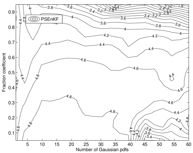
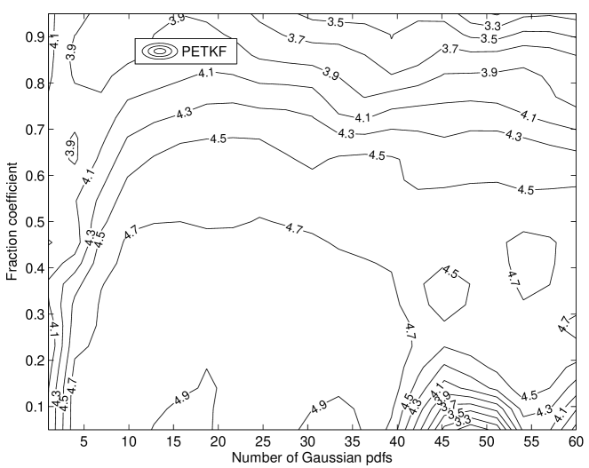
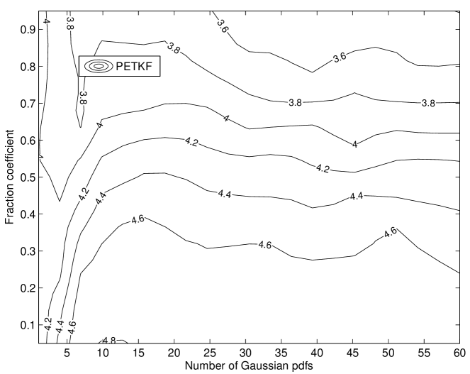
In Fig. 1 we show the rms errors of both the PSEnKF and PETKF as functions of the fraction coefficient and the number of Gaussian pdfs. First, we examine how the rmse of the PSEnKF changes with when is fixed. In Fig. 1(a), if is relatively small (say ), the rmse tends to decrease as increases. For larger (say ), the rmse of the filter exhibits the bell-shape behavior: at the beginning it increases when grows from ; after becomes relatively large (say ), further increasing reduces the rmse instead. Next, we examine the behavior of the rmse of the PSEnKF with respect to when is fixed. When is relatively small (say ), the rmse exhibits the U-turn behavior: at the beginning it intends to decrease as grows; after becomes relatively large (say ), further increasing increases the rmse instead. When is larger, say, , the rmse appears less sensitive to the change of . However, for even larger values of , say, , the rmse appears to monotonically decrease with .
The behavior of the PETKF (cf. Fig. 1(b)) with respect to the changes of and is similar to that of the PSEnKF. Therefore we do not repeat its description here.
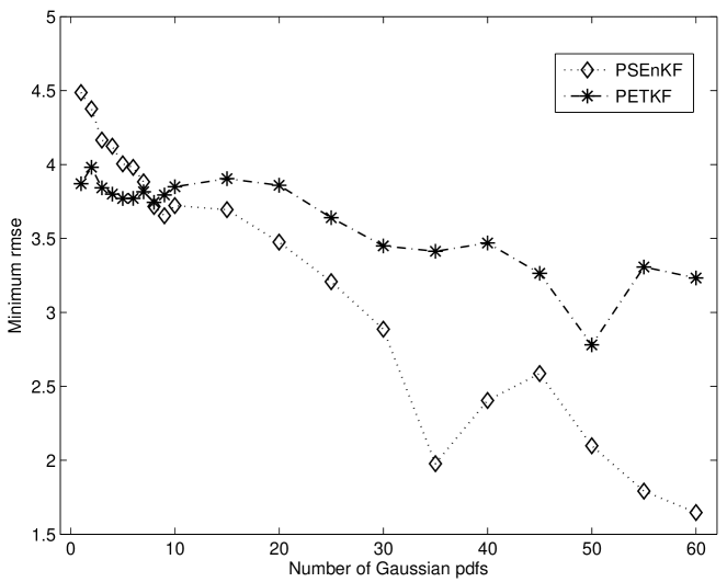
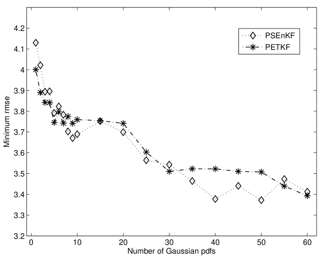
To examine the minimum rms errors of the PSEnKF and the PETKF within the tested values of and , we plot of both filters as functions of in Fig. 2. The of both filters tends to decrease as the number of Gaussian distributions increases, though there also exhibit certain local minima. The PSEnKF achieves its lowest at , while the PETKF at . As grows, both the PSEnKF and the PETKF tend to have lower than their corresponding base filters, the SEnKF and the ETKF (corresponding to the PSEnKF and the PETKF with , as discussed in § 3.2), respectively. This confirms the benefit of accuracy improvement by using the PEnKF instead of an EnKF. A comparison between the PSEnKF and the PETKF shows that the PETKF performs better than the PSEnKF when the number of Gaussian distributions is relatively small (say, ). However, as becomes larger, the PSEnKF outperforms its ETKF-based counterpart instead. Similar phenomena can also be observed in other experiments, as to be shown later.
4.3.2 Effect of the Ensemble Size
In the second experiment we examine the effect of the ensemble size of each SEnKF/ETKF in the PEnKF, on the performance of the PSEnKF/PETKF. For reference, we also examine the performance of the SEnKF and the ETKF under various ensemble sizes. The experiment settings are as follows. For the PSEnKF and the PETKF, we let the ensemble size of each EnKF take values from the set . For a single SEnKF/ETKF, we let , with two more values at and .
In the PSEnKF and the PETKF, we also vary the fraction coefficient such that . We fix the number of Gaussian pdfs, i.e., the number of ensemble filters, to be . To conduct covariance inflation, we let the inflation factor . We choose to conduct covariance localization, and set the length scale , only if the ensemble size is not larger than the dimension of the LE98 model. No covariance localization was conducted if . Our experience shows that, for , the benefit of conducting localization is not significant even if the length scale is properly chosen, while an improper value of is more likely to deteriorate the filter performance. To reduce statistical fluctuations, the experiments are again repeated for times.
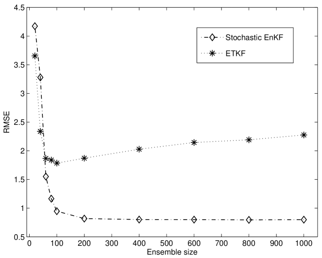
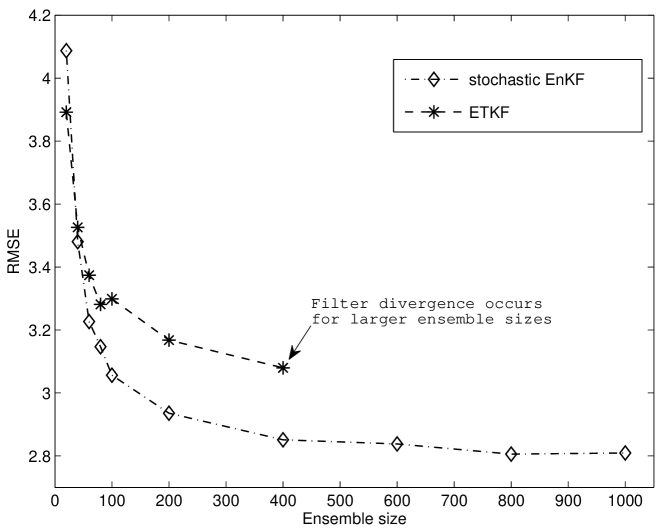
In Fig. 3 we show the rms errors of the SEnKF and the ETKF as functions of the ensemble size . The rmse of the ETKF exhibits a U-turn behavior. The rmse of the ETKF monotonically decreases as long as . Beyond that, the rmse monotonically increases instead as increases. On the other hand, the SEnKF exhibits a different behavior. Its rmse decreases for , and then reaches a plateau where the rmse remains almost unchanged as further increases.
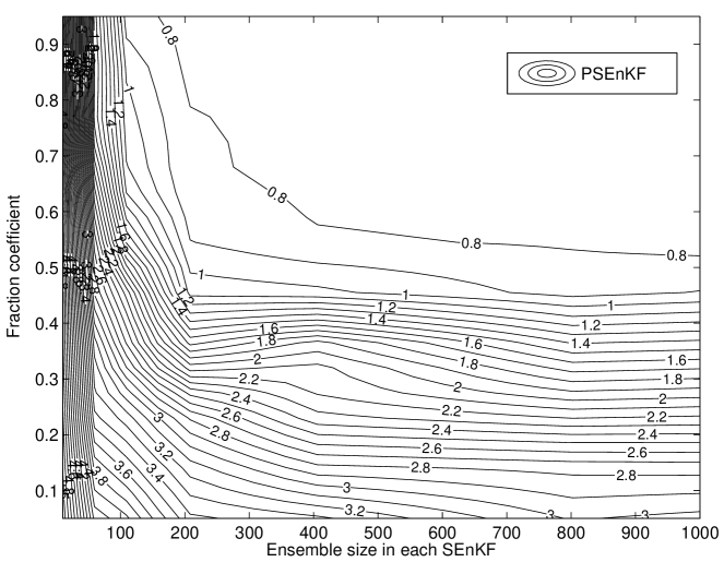
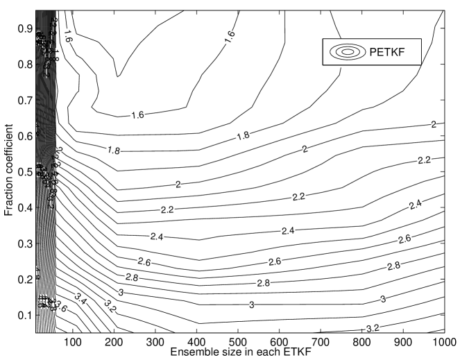
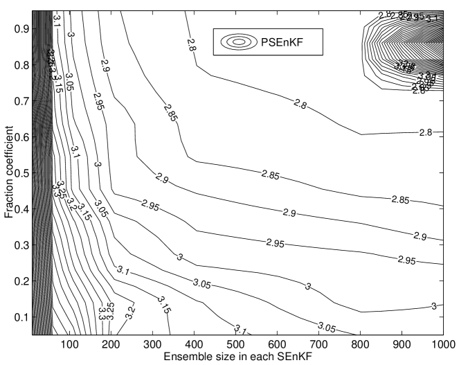
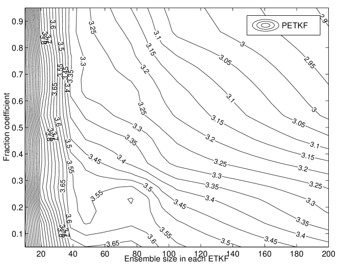
Fig. 4 plots the rms errors of the PSEnKF and the PETKF as functions of the fraction coefficient , and the ensemble size in the SEnKF and the ETKF used to construct the corresponding PEnKFs. The rms errors, as functions of the ensemble size (with fixed ), are consistent with our observations in Fig. 3. On the other hand, for both PEnKFs, their rms errors tend to decrease as the fraction coefficient increases.
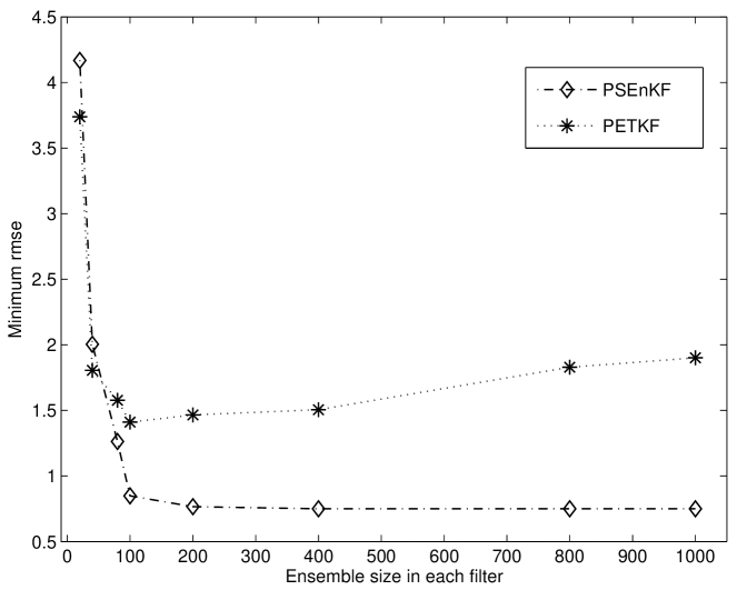
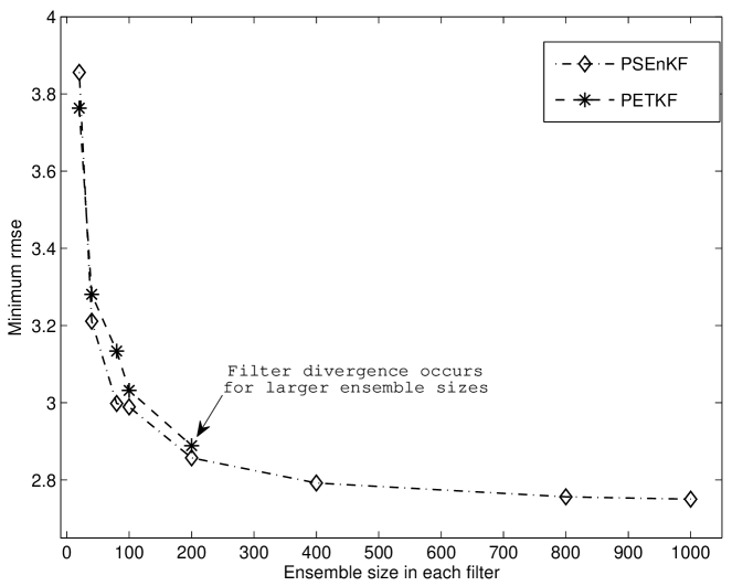
Per analogy to the first experiment, Fig. 5 plots the minimum rms errors of the PSEnKF and the PETKF within the tested fraction coefficient and the ensemble size . A comparison between Figs. 5 and 3 shows that, the minimum rms errors of the PEnKFs behave very similarly to the rms errors of their corresponding EnKFs in Fig. 3. Moreover, the values of in Fig. 5 tends to be lower than the corresponding rms errors in Fig. 3, indicating the benefit of accuracy improvement in using the PEnKFs. Again, a comparison between the PSEnKF and the PETKF shows that the PETKF performs better than the PSEnKF when the ensemble size is relatively small (say, ). However, as becomes larger, the PSEnKF outperforms the PETKF instead.
4.4 Experiments Results with a Nonlinear Observation Operator
In the second scenario, we introduce nonlinearity to the observation system. To this end, we let the observations be generated by the following nonlinear process
| (23) |
for every model time steps. In Eq. (23), again only the odd state variables () of the system state at time index are observed. The observation noise also follows the -dimensional Gaussian distribution . We conduct the same experiments as those in the case of linear observation operator.
4.4.1 Effect of the Number of Gaussian Distributions
We first examine the effect of the number of Gaussian distributions. The experiment settings are the same as those in § 4.3.1. Concretely, For either the PSEnKF or the PETKF, the number of Gaussian distributions , the fraction coefficient . For each individual SEnKF/ETKF in the PEnKF, the ensemble size , the covariance inflation factor and the length scale for covariance localization. As before, the experiments are repeated for times to reduce statistical fluctuations.
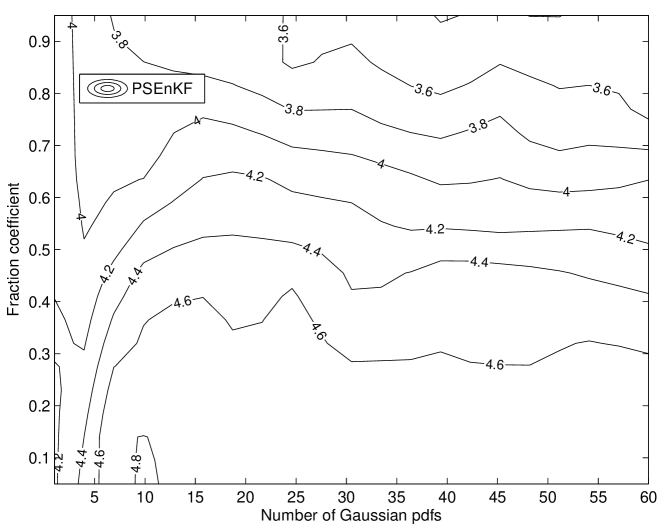
Fig. 6 plots the rms errors of both the PSEnKF and the PETKF as functions of the fraction coefficient and the number of Gaussian pdfs. When and changes, both the PSEnKF and the PETKF behave very similar to their counterparts in the linear case. The rms errors of the filters tend to decrease as increases, meaning that the PSEnKF/PETKF with in general performs better than the stochastic EnKF /ETKF (corresponding to the case in the PEnKF), consistent with the results obtained in the linear observer case.
We also examine the minimum rms errors of the PSEnKF and the PETKF within the tested values of and . Fig. 7 plots as functions of . For the PSEnKF, the lowest is achieved at . And for the PETKF, its tends to decrease within the tested range of , and achieves its minimum at . The PEnKF with more than one Gaussian distributions () performs better than the corresponding EnKF (). In addition, a comparison between the PSEnKF and the PETKF shows again that the PETKF performs better than the PSEnKF when the number of Gaussian distributions is relatively small, but tends to become worse as increases.
A comparison between Figs. 2 and 7 shows that the rmse of a filter (e.g. the PSEnKF at ) with a nonlinear observer sometimes may be lower than that of the same filter with a linear observer 222The result of comparison would also depend on the filter in use, its configuration, the system in assimilation, and so on, and therefore may change from case to case.. This seemingly counter-intuitive result happens possibly because in such situations, the effect of sampling error due to the relatively small ensemble size dominates the effect of nonlinearity in the observation system. However, as the number of Gaussian distributions increases, the effect of nonlinearity becomes more prominent so that the rmse with a nonlinear observer tends to be higher than that with a linear one. Similar phenomenon can also be found by comparing Figs. 3 and 5 with Figs. 8 and 10 (to be shown below), respectively, at different ensemble sizes.
4.4.2 Effect of the Ensemble Size
In the second experiment we examine the effect of the ensemble size in each ensemble filter on the performance of the corresponding PEnKF. For reference, we also examine the performance of the SEnKF and the ETKF under various ensemble sizes. The experiment settings are the same as those in § 4.3.2. In the PSEnKF and PETKF, we choose the fraction coefficient . We also choose the number of ensemble filters in each PEnKF to be . For each individual EnKF in the corresponding PEnKF, we let the ensemble size take values from the set , and for the experiments on the single EnKF, we let . To conduct covariance inflation and localization in each individual EnKF, we choose the inflation factor , and the length scale . As in § 4.3.2, covariance localization is conducted only if the ensemble size is no larger than the dimension .
Fig. 8 shows the rms errors of the SEnKF and the ETKF as functions of the ensemble size . For both filters, their rms errors decrease as the ensemble size increases. The ETKF performs better than the SEnKF in the small sample scenario with . But as increases, the SEnKF outperforms the ETKF instead. In particular, divergence in the ETKF occurs if , which did not happen in the linear observer case (cf. Fig. 3). On the other hand, the rmse of the SEnKF appears to reach a plateau for , similar to the linear observer case. Comparing Fig. 8 with Fig. 3, it is easy to see that, except for the stochastic EnKF at , the presence of nonlinearity in the observer deteriorates the performance of the ensemble filters.
Fig. 9 plots the rms errors of the PSEnKF and the PETKF as functions of the fraction coefficient , and the ensemble size in the corresponding SEnKF and the ETKF, respectively. In the PSEnKF (cf. Fig. 9(a)), the rmse tends to decrease as both and increases when the ensemble size . However, when , the impact of on the filter performance is not significant, which is consistent with the results in Fig. 8. On the other hand, in the PETKF (cf. Fig. 9(b)), filter divergence occurs for , which is why we only report its rmse with in Fig. 9(b), where the rmse of the PETKF appears to be a monotonically decreasing function of and .
In analogy to the first experiment, Fig. 10 plots the minimum rms errors of the PSEnKF and the PETKF within the tested fraction coefficient and ensemble size . One may observe that, similar to the SEnKF and the ETKF themselves, the of both the PSEnKF and the PETKF decrease as increases. However, for the PETKF, divergence occurs if , rather than as in Fig. 8, but overall its rmse is closer to that obtained in the PSEnKF. Meanwhile, a comparison between Fig. 8 and Fig. 10 shows that the PEnKFs perform better than the corresponding EnKFs. Also, a comparison between Fig. 5 and 10 shows that, except for the PSEnKF at , the nonlinearity in the observer again deteriorates the performance of the ensemble filters.
5 Discussion
This paper presented a discrete solution of the optimal nonlinear filter, called the particle Kalman filter (PKF), based on the Gaussian mixture representation of the state pdf given the observations. The PKF solves the nonlinear Bayesian correction step by complementing the Kalman filter-like correction step of the particles with a particle filter-like correction step of the weights. The PKF simultaneously runs a weighted ensemble of the Kalman filters in parallel. This is far beyond our computing capabilities when dealing with computationally demanding systems, as the atmospheric and oceanic models. Therefore, to reduce computational cost, one may instead consider a low-rank parametrization of the Gaussian mixture covariance matrices of the state pdfs. An efficient way to do that is to resort to the ensemble Kalman filter (EnKF) and use an EnKF-like method to update each component of the Gaussian mixture pdfs. This amounts to running a weighted ensemble of the EnKFs. In this work, the PKF was implemented using the stochastic EnKF and a deterministic EnKF, the ensemble transform Kalman filter (ETKF). We call this type of implementation the particle ensemble Kalman filter (PEnKF).
The PEnKF sets a nonlinear Bayesian filtering framework that encompasses the EnKF methods as a special case. As in the EnKF, the Kalman correction in the PEnKF attenuates the degeneracy of the ensemble by allocating the ensemble members far away from the incoming observation relatively more weights than in the particle filter, so that the filter can operate with reasonable size ensembles. To further improve the performance of the PEnKF, we also introduced to the PEnKF a re-sampling step similar to that used in the regularized particle filter (Musso et al., 2001; Stavropoulos and Titterington, 2001).
The stochastic EnKF and ETKF-based PEnKFs, called the PSEnKF and the PETKF, respectively, were implemented and their performance was investigated with the strongly nonlinear Lorenz-96 model. These filters were tested with both linear and nonlinear observation operators. Experiments results suggest that the PSEnKF and the PETKF outperform their corresponding EnKFs. It was also found that the ETKF outperforms the stochastic EnKF for small size ensembles while the stochastic EnKF exhibits better performance for large size ensembles. We argued that this happens because the EnKF endures less observational sampling errors when the ensemble size is large. Another reason would also be the better approximation of the PEnKF distributions provided by the stochastic EnKF compared to the ETKF. This was also true for their PEnKF counterparts. Overall, the conclusions from the numerical results obtained with the linear and nonlinear observation operators were not fundamentally different, except that in general better estimation accuracy was achieved with the linear observer when the sampling error is not the dominant factor. The results also suggest that the PEnKFs could more benefit from the use of more components in the mixture of normals (MON) and larger ensembles in the EnKFs in the nonlinear observations case.
Future work will focus on developing and testing new variants of the PEnKF that applies more efficient approximations, in term of computational cost, to update the mixture covariance matrices. Another direction for improvement would be also to work on localizing the correction step of the particle weights (Van Leeuwen, 2009). Our final goal is to develop a set of computationally feasible suboptimal PEnKFs that can outperform the EnKF methods at reasonable computational cost. As stated by Anderson (2003), developing filters in the context of the optimal nonlinear filtering problem, rather than starting from the Kalman filter, should lead to a more straightforward understanding of their capabilities.
The paper further discussed how the PEnKF can also be used as a general framework to simultaneously run several assimilation systems. We believe that this approach provides a framework to merge the solutions of different EnKFs, or to develop hybrid EnKF-variational methods. Work in this direction is under investigation.
Acknowledge
We would like to thank the three anonymous reviewers for their valuable comments and suggestions. Ibrahim Hoteit was partially supported by ONR grant N00014-08-1-0554.
References
- Anderson (2003) Anderson, J., 2003: A local least squares framework for ensemble filtering. Mon. Wea. Rev., 131 (4), 634–642.
- Anderson (2001) Anderson, J. L., 2001: An ensemble adjustment Kalman filter for data assimilation. Mon. Wea. Rev., 129, 2884–2903.
- Anderson and Anderson (1999) Anderson, J. L. and S. L. Anderson, 1999: A Monte Carlo implementation of the nonlinear filtering problem to produce ensemble assimilations and forecasts. Mon. Wea. Rev., 127, 2741–2758.
- Bengtsson et al. (2008) Bengtsson, T., P. Bickel, and B. Li, 2008: Curse-of-dimensionality revisited: Collapse of the particle filter in very large scale systems. IMS Collections, 2, 316–334.
- Bengtsson et al. (2003) Bengtsson, T., C. Snyder, and D. Nychka, 2003: Toward a nonlinear ensemble filter for high-dimensional systems. J. Geophys. Res., 108, 8775.
- Bishop et al. (2001) Bishop, C. H., B. J. Etherton, and S. J. Majumdar, 2001: Adaptive sampling with ensemble transform Kalman filter. Part I: theoretical aspects. Mon. Wea. Rev., 129, 420–436.
- Burgers et al. (1998) Burgers, G., P. J. van Leeuwen, and G. Evensen, 1998: On the analysis scheme in the ensemble Kalman filter. Mon. Wea. Rev., 126, 1719–1724.
- Chen and Liu (2000) Chen, R. and J. Liu, 2000: Mixture Kalman filters. Journal of the Royal Statistical Society: Series B (Statistical Methodology), 62 (3), 493–508.
- Doucet et al. (2001) Doucet, A., N. De Freitas, and N. Gordon, (Eds.) , 2001: Sequential Monte Carlo methods in practice. Springer Verlag.
- Evensen (1994) Evensen, G., 1994: Sequential data assimilation with a nonlinear quasi-geostrophic model using Monte Carlo methods to forecast error statistics. J. Geophys. Res., 99(C5), 10 143–10 162.
- Evensen and van Leeuwen (1996) Evensen, G. and P. J. van Leeuwen, 1996: Assimilation of geosat altimeter data for the aghulas current using the ensemble Kalman filter with a quasi-geostrophic model. Mon. Wea. Rev., 124, 85–96.
- Gaspari and Cohn (1999) Gaspari, G. and S. E. Cohn, 1999: Construction of correlation functions in two and three dimensions. Quart. J. Roy. Meteor. Soc., 125, 723 – 757.
- Ghil and Malanotte-Rizzoli (1991) Ghil, M. and P. Malanotte-Rizzoli, 1991: Data assimilation in meteorology and oceanography. Adv. Geophys, 33, 141–266.
- Hamill et al. (2009) Hamill, T. M., J. S. Whitaker, J. L. Anderson, and C. Snyder, 2009: Comments on “Sigma-point Kalman filter data assimilation methods for strongly nonlinear systems”. Journal of the Atmospheric Sciences, 66, 3498–3500.
- Hamill et al. (2001) Hamill, T. M., J. S. Whitaker, and C. Snyder, 2001: Distance-dependent filtering of background error covariance estimates in an ensemble Kalman filter. Mon. Wea. Rev., 129, 2776–2790.
- Han and Li (2008) Han, X. and X. Li, 2008: An evaluation of the nonlinear/non-Gaussian filters for the sequential data assimilation. Remote Sensing of Environment, 112, 1434 – 1449.
- Hoteit et al. (2002) Hoteit, I., D. T. Pham, and J. Blum, 2002: A simplified reduced order Kalman filtering and application to altimetric data assimilation in Tropical Pacific. Journal of Marine Systems, 36, 101–127.
- Hoteit et al. (2008) Hoteit, I., D. T. Pham, G. Triantafyllou, and G. Korres, 2008: A new approximate solution of the optimal nonlinear filter for data assimilation in meteorology and oceanography. Mon. Wea. Rev., 136, 317–334.
- Houtekamer and Mitchell (1998) Houtekamer, P. L. and H. L. Mitchell, 1998: Data assimilation using an ensemble Kalman filter technique. Mon. Wea. Rev., 126, 796–811.
- Jazwinski (1970) Jazwinski, A. H., 1970: Stochastic Processes and Filtering Theory. Academic Press.
- Kotecha and Djurić (2003) Kotecha, J. and P. Djurić, 2003: Gaussian particle filtering. Signal Processing, IEEE Transactions on, 51 (10), 2592–2601.
- Lorenz and Emanuel (1998) Lorenz, E. N. and K. A. Emanuel, 1998: Optimal sites for supplementary weather observations: Simulation with a small model. J. Atmos. Sci., 55, 399–414.
- Luo et al. (2010) Luo, X., I. M. Moroz, and I. Hoteit, 2010: Scaled unscented transform Gaussian sum filter: Theory and application. Physica D, 239, 684–701.
- Musso et al. (2001) Musso, C., N. Oudjane, and F. L. Gland, 2001: Improving regularized particle filters. Sequential Monte Carlo methods in practice, A. Doucet, N. de Freitas, and N. Gordon, Eds., Springer-Verlag, chap. 12, 247–271.
- Nakano et al. (2007) Nakano, S., U. G., and T. Higuchi, 2007: Merging particle filter for sequential data assimilation. Nonlin. Processes Geophys., 14, 395–408.
- Pham (2001) Pham, D. T., 2001: Stochastic methods for sequential data assimilation in strongly nonlinear systems. Mon. Wea. Rev., 129, 1194–1207.
- Redner and Walker (1984) Redner, R. and H. Walker, 1984: Mixture densities, maximum likelihood and the em algorithm. SIAM review, 26 (2), 195–239.
- Silverman (1986) Silverman, B. W., 1986: Density Estimation for Statistics and Data Analysis. Chapman & Hall.
- Simon (2006) Simon, D., 2006: Optimal State Estimation: Kalman, H-Infinity, and Nonlinear Approaches. Wiley-Interscience, 552 pp.
- Smith (2007) Smith, K. W., 2007: Cluster ensemble Kalman filter. Tellus, 59A, 749–757.
- Snyder et al. (2008) Snyder, C., T. Bengtsson, P. Bickel, and J. Anderson, 2008: Obstacles to high-dimensional particle filtering. Mon. Wea. Rev., 136, 4629–4640.
- Sorenson and Alspach (1971) Sorenson, H. W. and D. L. Alspach, 1971: Recursive Bayesian estimation using Gaussian sums. Automatica, 7, 465 – 479.
- Stavropoulos and Titterington (2001) Stavropoulos, P. and D. M. Titterington, 2001: Improved particle filters and smoothing. Sequential Monte Carlo methods in practice, A. Doucet, N. de Freitas, and N. Gordo, Eds., Springer-Verlag, chap. 14, 295–317.
- Todling (1999) Todling, R., 1999: Estimation theory and foundations of atmospheric data assimilation. 187 pp., DAO Office Note.
- Van Leeuwen (2003) Van Leeuwen, P. J., 2003: A variance minimizing filter for large-scale applications. Mon. Wea. Rev., 131, 2071–2084.
- Van Leeuwen (2009) Van Leeuwen, P. J., 2009: Particle filtering in geophysical systems. Mon. Wea. Rev., 137, 4089–4114.
- Whitaker and Hamill (2002) Whitaker, J. S. and T. M. Hamill, 2002: Ensemble data assimilation without perturbed observations. Mon. Wea. Rev., 130, 1913–1924.
- Xiong et al. (2006) Xiong, X., I. Navon, and B. Uzunoglu, 2006: A note on the particle filter with posterior Gaussian resampling. Tellus A, 58 (4), 456–460.
Support Material: The Full Re-sampling Algorithm
Here we discuss how to construct the ensemble set in the PEnKF. We note that the relative positions of the dimension of the random vector , the number of the Gaussian pdfs in the MON Eq. (13), and the ensemble size of each EnKF in the PKF determines our re-sampling strategies. In certain circumstances, a singular value decomposition (SVD) may be required on the covariance matrix in Eq. (14) such that
| (S.1) |
where is the matrix consisting of the eigenvectors of , and the diagonal matrix consisting of the corresponding eigenvalues (we also assume without loss of generality). Depending on the values of , and , one may avoid computing the full spectra of , as to be shown below.
Case I: and
In this case the number of (re-approximation) Gaussian distributions and the ensemble size are both less than the dimension of the system state. We consider two possibilities below.
Here we choose
| (S.2a) | ||||
| (S.2b) | ||||
The reason to choose the superscripts and on the right hand side of Eqs. (S.2a) and (S.2b) will be made clear soon. We also note that the sum
| (S.3) |
is not equal to exactly. Instead, it only adds up to the first terms of .
Let be the collection of the means in the MON , and
be the square root of in Eq. (S.2a), then it can be verified that
| (S.4) |
yields a set of the means that satisfy Eq. (S.2a), where denotes the transpose of the column vector with all its elements being one (so that consists of identical column vectors ), and is a matrix satisfying that , with being the -dimensional identity matrix, and that , with being a column vector with all its elements being zero. The first constraint, guarantees that the sample covariance of satisfies the constraint in Eq. (S.2a), and the second one, guarantees that the sample mean of is equal to , as is required in Eq. (16). For the generation of such a matrix , readers are referred to, for example, Hoteit et al. (2002); Pham (2001). In addition, since the dimension of is , we require that the dimension of the square root matrix is . Therefore, on the right hand side of Eq. (S.2a), the superscript shall be , rather than . The reason to use the superscript in Eq. (S.2b) is similar, as can be seen below.
To generate the ensembles (), with and being their sample means and covariances, we first construct the square root matrix
| (S.5) |
of , and generate by
| (S.6) |
where is a matrix similar to in Eq. (S.4). We note that the term is common to all EnKFs, and thus only needs to be calculated once. This is direct implication from the choice of the uniform covariance in , as we have pointed out previously, which leads to computational savings in comparison to the non-uniform choice.
Here we choose
| (S.7a) | ||||
| (S.7b) | ||||
Case II: and
In this case the number of Gaussian distributions is less than the dimension of the system state, but the ensemble size is larger than . We choose
| (S.10a) | ||||
| (S.10b) | ||||
The last equality in Eq. (S.10b) implies that one does not need to compute the full spectra of and the corresponding eigenvectors. Instead, one only needs to compute the first terms of .
Now define the square root matrix
| (S.11) |
so that one can again adopt Eq. (S.4) to generate (). To generate the ensembles , the situation here is different from that in the previous case, in that the ensemble size is larger than the dimension , so that one cannot obtain enough ensemble members through Eq. (S.6). As a result, one may instead choose to draw samples () from the distribution to form a matrix . Then the ensemble is produced via
| (S.12) |
Eq. (S.12) is similar to the partial re-sampling scheme in Hoteit et al. (2008), although here the perturbation term can be common to all EnKFs, and thus can be drawn only once to reduce computational cost.
Case III: and
In this case the ensemble size is no larger than the dimension of the system state, but the number of Gaussian distributions is. We choose
| (S.13a) | ||||
| (S.13b) | ||||
Since , we choose to draw samples from the distribution to form a matrix , while are generated by
| (S.14) |
Case IV: and
In this case both the number of Gaussian distributions and the ensemble size are larger than the dimension of the system state. We let and define . To generate , we first draw samples from the distribution to form a matrix , and then apply Eq. (S.14). Meanwhile, we also draw samples from the distribution to form a matrix , and then apply Eq. (S.12) to generate the ensembles .