Gravitational wave generation in loop quantum cosmology

Abstract

We calculate the full spectrum, as observed today, of the cosmological gravitational waves generated within a model based on loop quantum cosmology. It is assumed that the universe, after the transition to the classical regime, undergoes a period of inflation driven by a scalar field with a chaotic-type potential. Our analysis shows that, for certain conditions, loop quantum effects leave a clear signature on the spectrum, namely, an over-production of low-frequency gravitational waves. One of the aims of our work is to show that loop quantum cosmology models can be tested and that, more generally, pre-inflationary physical processes, contrary to what is usually assumed, leave their imprint in those spectra and can also be tested.

I Introduction

Although gravitational waves of cosmological origin have not yet been detected, they are at present the object of a considerable research effort, as they may provide us with a unique telescope to the earliest stages of the formation of the universe. At the same time we also witness an increasing interest in the applications of the ideas of loop quantum gravity (for a review, see Ref. rovelli-2008 ) to the problems of cosmology, a field known as loop quantum cosmology, interest that started after a series of seminal papers by Bojowald bojowald-varios , where a number of important results were obtained, among them the possibility of removing in a natural way the presence of the cosmological singularity (for a review about loop quantum cosmology, see Ref. bojowald-2008 ).

Tests of loop quantum cosmology have already been proposed bojowald-lidsey-mulryne-singh-tavakol ; tsujikawa-singh-maartens ; hossain ; copeland-mulryne-nunes-shaeri ; bojowald-calcagni ; bojowald-calcagni-tsujikawa-A ; bojowald-calcagni-tsujikawa-B , showing that loop effects may appear, albeit in an indirect way, on the cosmic microwave background radiation on the largest scales. Loop quantum cosmology gives rise to changes in the dynamical equations driving the expansion of the universe; these are connected with modifications in the equation of state of the matter content of the universe, which in turn result in the production of gravitational waves. These gravitational waves are the focus of our work, where we show that they may leave an important imprint in today’s power spectrum. This at first may seem surprising, as it has usually been assumed that inflation, by its characteristics, among them the enormous increase in the scale of the universe, would remove any kind of information coming from physical phenomena taking place in pre-inflationary times. This is not the case. Pre-inflationary physical features affect in a different way different frequencies and the memory of such differences survives through the inflationary period, and can be read today in the power spectrum.

Our paper is organized as follows. In the next section we describe the loop quantum cosmology model used in our work and write the equations of motion for the semiclassical and classical stages of evolution of the universe. Taking into account the constraints arising from measurements of the cosmic microwave background radiation, we specify the values of the parameters and the initial conditions and solve numerically the evolutionary equations, from the semiclassical pre-inflationary epoch till the present time. In Section III we calculate the full gravitational-wave spectrum, for frequencies ranging from about $10^{-17}$ rad/s to about $10^{9}$ rad/s, using the method of continuous Bogoliubov coefficients. The influence on the spectrum of the ambiguity parameters of loop quantum cosmology is carefully analyzed. In section IV we summarize the results we have obtained.

II The evolution of the universe

The evolution of the universe is naturally divided in two stages, corresponding to the semiclassical and the classical regimes. During the semiclassical stage of evolution, the equations of standard cosmology have to be modified in order to account for loop quantum effects. After a few Planck times of evolution, the transition between the semiclassical and classical regimes takes place and the universe further evolves according to the standard cosmological model, namely, undergoes a period of inflation, driven by a scalar field $\phi$ with chaotic-type potential

$$V(\phi)=\frac{1}{2}m_{\phi}^{2}\phi^{2},$$ (1)

followed by reheating and, successively, by radiation-dominated, matter-dominated and dark energy-dominated periods.

During the semiclassical stage, the modified evolutionary equations for the scale factor $a$ and the scalar field $\phi$ are given by tsujikawa-singh-maartens ; mielczarek-szydlowski ; grain-et-al

$$\left(\frac{\dot{a}}{a}\right)^{2}=\frac{8\pi}{3m_{\textsc{P}}^{2}}\left[\frac{\dot{\phi}^{2}}{2D(q)}+V(\phi)\right],$$ (2)

$$\frac{\ddot{a}}{a}=\frac{8\pi}{3m_{\textsc{P}}^{2}}\left[V(\phi)-\frac{\dot{\phi}^{2}}{D(q)}\right]+\frac{2\pi\dot{\phi}^{2}}{m_{\textsc{P}}^{2}}\frac{F(q)}{D(q)},$$ (3)

$$\ddot{\phi}=-3\frac{\dot{a}}{a}\Big{[}1-F(q)\Big{]}\dot{\phi}-D(q)\frac{\partial V}{\partial\phi},$$ (4)

where a flat Friedmann-Robertson-Walker background is assumed, $m_{\textsc{P}}$ is the Planck mass, a dot denotes a derivative with respect to the cosmic time $t$ and the following notation was introduced bojowald-2004

$$D(q) = \left(\frac{3}{2\ell}\right)^{\frac{3}{2-2\ell}}q^{3/2}\left\{\frac{1}{\ell+2}\Big{[}(q+1)^{\ell+2}-|q-1|^{\ell+2}\Big{]}\right.$$ (5)

$$\left.-\frac{q}{\ell+1}\Big{[}(q+1)^{\ell+1}-\mbox{sign}(q-1)|q-1|^{\ell+1}\Big{]}\right\}^{\frac{3}{2-2\ell}},$$

and

$$F(q) = \frac{1}{\ell-1}\Big{\{}(\ell^{2}-1)\Big{[}(q+1)^{\ell+2}-|q-1|^{\ell+2}\Big{]}$$ (6)

$$-(2\ell-1)(\ell+2)q\Big{[}(q+1)^{\ell+1}-\mbox{sign}(q-1)|q-1|^{\ell+1}\Big{]}$$

$$+(\ell+1)(\ell+2)q^{2}\Big{[}(q+1)^{\ell}-|q-1|^{\ell}\Big{]}\Big{\}}$$

$$\times\Big{\{}(\ell+1)\Big{[}(q+1)^{\ell+2}-|q-1|^{\ell+2}\Big{]}$$

$$-(\ell+2)q\Big{[}(q+1)^{\ell+1}-\mbox{sign}(q-1)|q-1|^{\ell+1}\Big{]}\Big{\}}^{-1},$$

with

$$q=\left(\frac{a}{a_{*}}\right)^{2},\quad a_{*}=\sqrt{\frac{\gamma j}{3}}\,\ell_{\textsc{P}},\quad\gamma=0.2375.$$ (7)

In the above expressions $\ell$ and $j$ are the so-called ambiguity parameters and $\ell_{\textsc{P}}$ denotes the Planck length.

Equations (3) and (4) are solved numerically for the following values of the parameters and the initial conditions: $m_{\phi}=10^{-6}\,m_{\textsc{P}}$, $a_{i}=\sqrt{\gamma}\,\ell_{\textsc{P}}$, $\phi_{i}=3.6\times 10^{11}j^{-15/2}m_{\textsc{P}}$ and $\dot{\phi}_{i}=2\times 10^{-6}\,m_{\textsc{P}}^{2}$, with $\dot{a}_{i}$ being fixed by Eq. (2). This equation is also used to check the accuracy of the numerical solution. The initial value for scalar field was chosen such that the uncertainty principle tsujikawa-singh-maartens ,

$$|\phi_{i}\dot{\phi}_{i}|\gtrsim\frac{10^{3}}{j^{3/2}}\left(\frac{a_{i}}{a_{*}}\right)^{12}m_{\textsc{P}}^{3},$$ (8)

is marginally satisfied.

The ambiguity parameter $\ell$ is quantized, taking values

$$\ell=1-\frac{1}{2n};\quad n\in\mathbb{N}.$$ (9)

The other ambiguity parameter, $j$, takes half-integer values greater than one. However, if one demands the initial value of the scalar field, $\phi_{i}$, to be much smaller than the Planck mass (say, $\phi_{i}\lesssim 10^{-3}\,m_{\textsc{P}}$), then the parameter $j$ is constrained to be much bigger than one, namely, $j\gtrsim 87.3$. In what follows, we will consider $j$ to be a continuously varying parameter with values greater or of the order of $100$.

As our numerical calculations show, after a short period of time, the functions $D(q)$ e $F(q)$ approach their classical values, namely, $D=1$ and $F=0$, and the semiclassical corrections can be neglected in Eqs. (2)–(4). The resulting simplified evolutionary equations are then solved up to the end of the inflationary period.

At the end of the semiclassical stage of evolution, the scalar field increases from a small value (much smaller than the Planck mass) to a value of the order of one Planck mass (see Fig. 1). This is due to the fact that the first term on the right-hand-side of Eq. (4) acts as an anti-friction term, pushing the scalar field up the potential. During the subsequent classical stage of evolution, the scalar field continues to increase for a while, reaching a maximum value of about $3\,m_{\textsc{P}}$ (for $j=100$ and $\ell=3/4$). This value of $\phi_{\mbox{\scriptsize{max}}}$ is enough for the universe to expand about $60$ $e$-folds during the inflationary period. Therefore, loop quantum effects can set the initial conditions for successful chaotic inflation in a natural way tsujikawa-singh-maartens .

Figure 1: Time evolution of the scalar field $\phi$ for the case $j=100$ and $\ell=3/4$. Because of loop quantum effects, the scalar field increases naturally from its initial value of about $3.6\times 10^{-4}\,m_{\textsc{P}}$ to a maximum value of about $3\,m_{\textsc{P}}$, which guarantees a long enough inflationary period.

At the end of the inflationary period, the scalar field begins to oscillate around the minimum of the potential, transferring its energy to a radiation fluid, thus reheating the universe. The decay of the scalar field into radiation is governed by a dissipative coupling introduced in the evolutionary equations, which now read

$$\left(\frac{\dot{a}}{a}\right)^{2}=\frac{8\pi}{3m_{\textsc{P}}^{2}}\left[\frac{\dot{\phi}^{2}}{2}+V(\phi)+\rho_{r}\right],$$ (10)

$$\frac{\ddot{a}}{a}=\frac{8\pi}{3m_{\textsc{P}}^{2}}\left[V(\phi)-\dot{\phi}^{2}-\rho_{r}\right],$$ (11)

$$\ddot{\phi} = -3\frac{\dot{a}}{a}\dot{\phi}-\frac{\partial V}{\partial\phi}-\Gamma_{\phi}\dot{\phi},$$ (12)

$$\dot{\rho_{r}}=-4\frac{\dot{a}}{a}\rho_{r}+\Gamma_{\phi}\dot{\phi}^{2},$$ (13)

where $\rho_{r}$ is the energy density of radiation and $\Gamma_{\phi}$ is the dissipative coefficient. Since any preexisting radiation fluid would have been diluted during the inflationary period, we choose the energy density of radiation at the beginning of reheating to be zero, $\rho_{r,i}=0$. For the dissipative coefficient we choose $\Gamma_{\phi}=2\times 10^{-7}m_{\textsc{P}}$.

After a while, the energy density of the scalar field becomes much smaller than the energy density of radiation, meaning that the former can be consistently neglected. The evolutionary equations then become

$$\left(\frac{\dot{a}}{a}\right)^{2}=\frac{8\pi G}{3c^{2}}\left[\rho_{r,0}\left(\frac{a_{0}}{a}\right)^{4}+\rho_{m,0}\left(\frac{a_{0}}{a}\right)^{3}\right.$$

$$+\left.\rho_{de,0}\left(\frac{a_{0}}{a}\right)^{3(w+1)}\right],$$ (14)

$$\frac{\ddot{a}}{a}=-\frac{4\pi G}{3c^{2}}\left[2\rho_{r,0}\left(\frac{a_{0}}{a}\right)^{4}+\rho_{m,0}\left(\frac{a_{0}}{a}\right)^{3}\right.$$

$$+\left.(3w+1)\rho_{de,0}\left(\frac{a_{0}}{a}\right)^{3(w+1)}\right],$$ (15)

where $a_{0}$ is today’s value of the scale factor and $\rho_{r,0}=4.13\times 10^{-14}\mbox{ J/m}^{3}$, $\rho_{m,0}=2.34\times 10^{-10}\mbox{ J/m}^{3}$ and $\rho_{de,0}=6.20\times 10^{-10}\mbox{ J/m}^{3}$ are, respectively, today’s values of the energy density of radiation, matter, and dark energy. For these values of $\rho_{r,0}$, $\rho_{m,0}$, and $\rho_{de,0}$, the value of the Hubble constant is $H_{0}=71\mbox{ km s}^{-1}\mbox{Mpc}^{-1}$. We take the value $w=-1$ for the equation-of-state parameter of dark energy.

To finish this section, let us point out that for a given value of $j$, the requirement that the universe expands enough during the inflationary period (at least $60$ $e$-folds), imposes a lower bound on the value of $\ell$ (see Fig. 2).

Figure 2: The shaded region corresponds to values of the ambiguity parameters $\ell$ and $j$ for which the universe expands at least $60$ $e$-folds during the inflationary period. Such an expansion is achieved if the scalar field grows from $\phi_{i}\ll\,m_{\textsc{P}}$ to $\phi_{\mbox{\scriptsize max}}\gtrsim 3\,m_{\textsc{P}}$ during the pre-inflationary epoch. The requirement that $\phi_{i}\lesssim 10^{-3}m_{\textsc{P}}$, together with the choice $m_{\phi}=10^{-6}\,m_{\textsc{P}}$ and $\dot{\phi}_{i}=2\times 10^{-6}\,m_{\textsc{P}}^{2}$, imposes the constraint $j\gtrsim 87.3$.

III The gravitational-wave spectrum

Gravitational waves are generated in an expanding universe, giving rise to a spectrum extending over a wide range of frequencies grishchuk74 ; starobinskii79 ; abbott-harari ; Allen88 ; sahni ; grishchuk-solokhin ; allen97 . In this section we calculate the full spectrum of the gravitational waves generated within the loop quantum cosmology model described above.

Loop quantum effects introduce modifications not only to the dynamical equations of evolution (2)–(4), but also to the equation for tensor modes. However, in this paper, the latter will be neglected, allowing for a considerable simplification of the calculations required to determine the energy spectrum of gravitational waves, while keeping unchanged the main features of the spectrum.

The tensor perturbations $h_{ij}$ to the Friedmann-Robertson-Walker metric,

$$ds^{2}=a^{2}(\eta)\left\{-d\eta^{2}+\left[\delta_{ij}+h_{ij}(\eta,\textbf{x})\right]dx^{i}dx^{j}\right\},$$ (16)

can be expanded in terms of plane waves

$$h_{ij}(\eta,\textbf{x})=\sqrt{8\pi G}\sum\limits_{p=1}^{2}\int\frac{d^{3}k}{(2\pi)^{3/2}a(\eta)\sqrt{2k}}$$

$$\times\left[a_{p}(\eta,{\bf k})\varepsilon_{ij}(\textbf{k},p)e^{i\textbf{k}\cdot\textbf{x}}\xi(\eta,k)+\mbox{H.c.}\right],$$ (17)

where $G$ is the gravitational constant, $p$ runs over the two polarizations of the gravitational waves, $k=|\textbf{k}|=2\pi a/\lambda=a\omega$ is the co-moving wave number, $a_{p}$ is the annihilation operator, and $\varepsilon_{ij}$ is the polarization tensor. The mode function $\xi(\eta,k)$ obeys the equation of a parametric oscillator,

$$\xi^{\prime\prime}+\left(k^{2}-U\right)\xi=0,$$ (18)

where the potential $U$ is given by

$$U=\frac{a^{\prime\prime}}{a}$$ (19)

and a prime denotes a derivative with respect to conformal time $\eta$.

For $k^{2}\lesssim U$, the above equation describes the production of gravitational waves with frequency $\omega=k/a$, while for $k^{2}\gg U$ the equation is that of an harmonic oscillator, implying that no gravitational waves are produced.

Within the standard model of cosmology, the potential $U$ has a pronounced barrier at the time of inflation, giving rise to a copious production of gravitational waves with frequencies up to the gigahertz. Within loop quantum cosmology, besides the above mentioned inflationary barrier, the potential $U$ has another barrier at very early times (see Fig. 3). The presence of this barrier leads to the creation of extra gravitational waves of low frequency. This barrier is slightly more pronounced, if one takes into account loop quantum corrections to the equation of tensor perturbations.

Figure 3: Potential $U$ as a function of (cosmic) time $t$ for the case $\ell=3/4$ and $j=100$. The inflationary barrier is located on the right (for $t\gtrsim 10^{6}t_{\textsc{P}}$), while the much smaller barrier arising due to loop quantum effects is located on the left (for $t\lesssim t_{\textsc{P}}$).

In order to calculate the energy spectrum of the cosmological gravitational waves generated during the evolution of the universe, from the semiclassical pre-inflationary stage of evolution till the present time, we use the method of continuous Bogoliubov coefficients. This method, first applied by Parker parker to particle production in an expanding universe and then extended to the case of gravitons henriques94 ; henriques-moorhouse-mendes ; mendes-henriques-moorhouse , can be summarized as follows (for applications of this method to several cosmological models see Refs. henriques04 ; sa-henriques1 ; sa-henriques2 ; sa-henriques-potting ; sa-henriques3 ).

The gravitational-wave spectral energy density parameter, $\Omega_{\textsc{gw}}$, is defined as

$$\Omega_{\textsc{gw}}=\frac{8\hbar G}{3\pi c^{5}H_{0}^{2}}\omega_{0}^{4}\beta_{0}^{2},$$ (20)

where $\hbar$ is the reduced Planck constant, $G$ is the gravitational constant, $c$ is the speed of light, $H$ is the Hubble parameter, $\omega$ is the gravitational-wave frequency, $\beta$ is a Bogoliubov coefficient and the subscript $0$ denotes quantities evaluated at the present time.

The angular frequency $\omega_{0}$ takes values ranging from about $1.4\times 10^{-17}\mbox{ rad/s}$ (corresponding to a wavelength equal, today, to the Hubble distance) to about $10^{9}\mbox{ rad/s}$ (corresponding to a wavelength equal to the Hubble distance at the end of the inflationary period).

The number of gravitons at a certain time is given by the squared Bogoliubov coefficient,

$$|\beta(t)|^{2}=\frac{1}{4}[X(t)-Y(t)][X^{*}(t)-Y^{*}(t)],$$ (21)

where $*$ denotes complex conjugate and the functions $X$ and $Y$ are solutions of the system of differential equations

$$\dot{X}=-i\frac{\omega_{0}a_{0}}{a}Y,$$ (22)

$$\dot{Y}=-i\frac{a}{\omega_{0}a_{0}}\left[\left(\frac{\omega_{0}a_{0}}{a}\right)^{2}-\frac{\ddot{a}}{a}-\left(\frac{\dot{a}}{a}\right)^{2}\right]X,$$ (23)

which is integrated with initial conditions $X(t_{i})=Y(t_{i})=1$, corresponding to the absence of gravitons at the beginning of the evolution. In the above system of differential equations, the scale factor, $a(t)$, and its first and second derivatives, $\dot{a}(t)$ and $\ddot{a}(t)$, are determined from the evolutionary equations presented in the previous section, namely, Eqs. (2)–(4) for the semiclassical stage of evolution and the inflationary period , (10)–(13) for the reheating period, and (14)–(15) for the radiation-dominated, matter-dominated and dark energy-dominated periods.

Using the above outlined method of continuous Bogoliubov coefficients, we can calculate the gravitational-wave spectrum for different values of the ambiguity parameters $j$ and $\ell$. Let us first analyze the case of fixed $j$ (say, $j=100$) and varying $\ell$.

Figure 4: Gravitational-wave spectra for $\ell=3/4$ and $\ell=5/6$ (dashed line). In both cases $j=100$.

For $\ell=3/4$, loop quantum effects leave a clear signature on the spectrum, namely, an over-production of low-frequency gravitational waves (see Fig. 4). For $\ell=5/6$ the spectrum shows no influence of these effects. This can be understood as follows. Today’s frequency of a gravitational wave that crossed the Hubble horizon at time $t$ is given by $2\pi H(t)[a(t)/a(t_{0})]$. For $\ell=3/4$, gravitational waves generated in the early universe ($t\lesssim 10^{5}\,t_{\textsc{P}}$) have frequencies, today, of the order of $(10^{-11}-10^{-17})\mbox{ rad/s}$, corresponding to wavelengths of the order or smaller than the Hubble horizon today (see Fig. 5). Therefore, these gravitational waves leave their imprint on the spectrum at low frequencies. For $\ell=5/6$, gravitational waves generated in the early universe have, today, frequencies of the order of $(10^{-38}-10^{-45})\mbox{ rad/s}$, corresponding to wavelengths much bigger than the Hubble horizon today. Therefore, these gravitational waves leave no imprint on the spectrum. Note that in the case $\ell=3/4$ the scale factor grows about $60$ $e$-folds during the inflationary period, while in the case $\ell=5/6$ the growth of the scale factor is about $140$ $e$-folds.

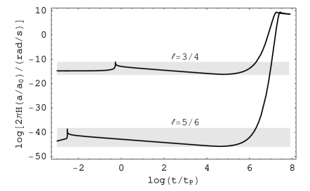
Figure 5: Today’s frequency of a gravitational wave as a function of the time at which this wave first crossed the Hubble horizon. For $\ell=3/4$, gravitational waves generated in the early universe have frequencies, today, of the order of $(10^{-11}-10^{-17})\mbox{ rad/s}$ (shaded region), corresponding to wavelengths of the order or smaller than the Hubble horizon today. For $\ell=5/6$, gravitational waves generated in the early universe have, today, frequencies of the order of $(10^{-38}-10^{-45})\mbox{ rad/s}$, corresponding to wavelengths much bigger than the Hubble horizon today. For both cases today’s maximum frequency of the gravitational waves is of the order of $10^{9}\mbox{ rad/s}$, corresponding to waves that crossed the Hubble horizon at the end of the inflationary period ($t\sim 3\times 10^{7}\,t_{\textsc{P}}$).

For the case $j=2000$ the situation is similar to the one described above (see Fig. 6). Loop quantum effects leave an imprint on the gravitational-wave spectrum only if the ambiguity parameter $\ell$ takes such a value ($\ell=1/2$) that the universe expands about $60$ $e$-folds during the inflationary period. If the universe expands much more than $60$ $e$-folds (for instance, in the case $\ell=3/4$ the scale grows about $240$ $e$-folds), the gravitational waves generated before the inflationary period have wavelengths, today, much bigger than the Hubble horizon and, consequently, they leave no imprint on the gravitational-wave energy spectrum.

Figure 6: Gravitational-wave spectra for $\ell=1/2$ and $\ell=3/4$ (dashed line). In both cases $j=2000$.

We have been assuming that the ambiguity parameter $\ell$ is quantized, taking values $\ell=1-1/(2n)$, with $n\in\mathbb{N}$. If, however, we consider $\ell$ to be a free parameter, changing continuously from $0$ to $1$, then our conclusions need to be slightly adapted. Namely, for each value of $j$ there is a critical value of the ambiguity parameter, $\ell_{\mbox{\scriptsize crit}}$, for which the universe expands $60$ $e$-folds during the inflationary period, the minimum required in standard inflationary cosmology. For values of $\ell$ close to $\ell_{\mbox{\scriptsize crit}}$, the gravitational waves generated during the pre-inflationary epoch leave an imprint on the spectrum at low frequencies. As we (continuously) increase $\ell$, this imprint shows up at lower and lower frequencies, completely disappearing when today’s frequency of the generated waves is so low ($\omega_{0}\lesssim 10^{-17}\mbox{ rad/s}$), that it corresponds to a wavelength greater than the Hubble horizon. On the contrary, if we consider values of $\ell$ smaller than the critical one (in which case the scale factor does not grow enough during the inflationary period), the imprint of the pre-inflationary gravitational waves appears on the spectrum at higher frequencies.

The above conclusions are illustrated in Fig. 7. For $j=100$ the critical value of the ambiguity parameter $\ell$ is about $0.75$ (see Fig. 2). In this case, loop quantum effects leave their signature on the spectrum at frequencies $\omega_{0}\lesssim 10^{-12}\mbox{ rad/s}$. For $\ell=0.70$ and $\ell=0.73$ the gravitational waves generated prior to the inflationary period leave an imprint at frequencies higher than in the critical case, $\omega_{0}\lesssim 10^{-5}\mbox{ rad/s}$ and $\omega_{0}\lesssim 10^{-8}\mbox{ rad/s}$, respectively. However, for such values of the ambiguity parameters, the scale factor grows about $45$ and $54$ $e$-folds, respectively, during the inflationary period, which is less than required by standard inflationary cosmology. For the $\ell=0.77$ (above $\ell_{\mbox{\scriptsize crit}}=0.75$) the signature of loop quantum cosmology is located at frequencies lower than in the critical case, $\omega_{0}\lesssim 10^{-16}\mbox{ rad/s}$. In this case, the scale factor grows about $71$ $e$-folds during the inflationary period.

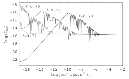
Figure 7: Gravitational-wave spectra for $\ell=0.70$, $0.73$, $0.75$ and $0.77$ ($j=100$ in all cases). Loop quantum effects leave a signature on the spectra, namely, an over-production of gravitational waves at low frequencies. As $\ell$ increases this signature is located at increasingly lower frequencies. For $\ell=0.77$ the signature moved to frequencies so low, that it becomes almost unnoticeable in the spectrum.

To conclude, let us compare gravitational-wave spectra for a fixed value of $\ell$ (say, $\ell=0.6$) and varying $j$. For $\ell=0.6$, enough growth of the scale factor during the inflationary period is guaranteed for $j\gtrsim 560$ (see Fig. 2). Therefore, as expected, for $j=560$ loop quantum effects leave their imprint at low frequencies, $\omega_{0}\lesssim 10^{-11}\mbox{ rad/s}$ (see Fig. 8). For $j=750$ the loop quantum signature moves to lower frequencies, $\omega_{0}\lesssim 10^{-14}\mbox{ rad/s}$, while for $j=100$ it moves to higher frequencies, $\omega_{0}\lesssim 10\mbox{ rad/s}$. In the latter case, the imprint of loop quantum cosmology lies in the frequency band accessible to the Laser Interferometer Space Antenna (LISA) and, in principle, could be seen by this detector. Note, however, that the growth of the scale factor during the inflationary period in this case is just about $28$ $e$-folds, which is manifestly insufficient within standard inflationary cosmology.

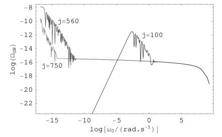
Figure 8: Gravitational-wave spectra for $j=100$, $560$ and $750$ ($\ell=0.6$ in all cases). As $j$ increases the loop quantum signature shows up at increasingly lower frequencies.

To finish this section, let us point out that measurements of the cosmic microwave background radiation can be used to derive an upper limit on the gravitational-wave spectral energy density parameter, namely, $\Omega_{\textsc{gw}}<1.4\times 10^{-10}$ for $\omega_{0}=1.4\times 10^{-17}\mbox{ rad/s}$ allen97 . Some gravitational-wave spectra shown in this paper do not satisfy this bound. Taking into account that the inflaton mass $m_{\phi}$ determines the overall vertical displacement of the gravitational-wave spectrum, one just needs to consider lower values of $m_{\phi}$ in order to make these spectra compatible with the above mentioned upper limit.

IV Conclusions

In this work we have investigated the generation of gravitational waves within loop quantum cosmology models. For such models, the evolution of the universe is naturally divided in two stages, corresponding to the semiclassical and the classical regimes. In the former, loop quantum effects introduce modifications to the dynamical equations describing the evolution of the early universe, while in the latter the evolution proceeds according to the usual general relativity equations. The transition between the two regimes takes place at very early times.

For the semiclassical regime we have assumed that the corrections to the dynamical equations are of the inverse-volume type, leaving for a future investigation the holonomy corrections. Inverse-volume corrections involve two ambiguity parameters, $j$ and $\ell$, which we have assumed to be free parameters.

For the classical regime, we have assumed that the evolution of the universe proceeds according to the usual standard inflationary model, i.e., a inflationary epoch (of the chaotic type) is followed by reheating and then, successively, by radiation-dominated, matter-dominated and dark energy-dominated periods of evolution.

We have also assumed that, initially, the inflaton field $\phi$ is located near the origin of the chaotic-type potential, taking values much smaller than the Planck mass. This choice of initial conditions is admissible, since loop quantum corrections to the dynamical equations guarantee that the scalar field $\phi$ is pushed up the potential, reaching maximum values of the order of the Planck mass at the beginning of the inflationary period (see Fig. 1), which is required to obtain enough inflation.

The assumption that $\phi_{i}\ll m_{\textsc{P}}$ and $\dot{\phi}_{i}\ll m_{\textsc{P}}^{2}$, together with the requirement that initially the scalar field satisfies marginally the uncertainty principle, imposes a lower bound on the value of the ambiguity parameter $j$, namely, $j\gtrsim 100$. Another constraint on the values of $j$ and $\ell$ comes from the requirement that the scale factor grows at least $60$ $e$-folds during the inflationary period. Our numerical calculations show that this condition is satisfied just for the values of the ambiguity parameters $j$ and $\ell$ corresponding to the shaded region of Fig. 2.

Loop quantum effects introduce modifications not only to the dynamical equations describing the evolution of the universe, but also to the equation of tensor modes. However, in this paper, we have taken into account only the modifications to the dynamical equations, thus simplifying considerably the calculations without loosing the main features of the gravitational-wave energy spectrum.

To calculate the full gravitational-wave energy spectrum we have used the method of continuous Bogoliubov coefficients. Our analysis shows that, for certain conditions, loop quantum effects leave a clear signature on the spectrum, namely, an over-production of low-frequency gravitational waves. This signature is present on the gravitational-wave spectrum only if the growth of the scale factor during the inflationary period does not exceed significantly the minimum growth required in standard inflationary cosmology, namely, $60$ $e$-folds. If the scale factor grows much more than this value, gravitational waves generated prior to the inflationary period have, today, a wavelength much bigger than the Hubble horizon, leaving no imprint on the gravitational-wave spectrum. On the other hand, if the growth of the scale factor during the inflationary period is smaller than $60$ $e$-folds, then the imprint of loop quantum cosmology is clearly seen on the gravitational-wave spectrum, at frequencies which increase with decreasing number of $e$-folds of expansion during inflation. For example, in the case $\ell=0.6$ and $j=100$, for which about $28$ $e$-folds of expansion are obtained during inflation, loop quantum effects leave their signature at LISA frequency band. Taken into account the above comments, we conclude that the values of the ambiguity parameters $j$ and $\ell$ for which a signature of loop quantum cosmology shows up on the gravitational-wave spectrum are those corresponding to a narrow band around the thick line of Fig. 2, i.e., these values for which the scale factor grows about $60$ $e$-folds during the inflationary period.

Our results shows that, contrary to what is usually assumed, inflation does not necessarily erase all the information on physical features present in the pre-inflationary era. Indeed, as we have shown, within loop quantum cosmology physical processes taking place in the very early universe, prior to the inflationary period, leave their imprint on the spectrum of the gravitational waves at very low frequencies, corresponding to wavelengths of the order of the Hubble distance. Despite the fact that the gravitational-wave spectral energy density parameter $\Omega_{\textsc{gw}}$ for such frequencies may be quite high, a direct detection is not possible. Nevertheless, these gravitational waves may have left their imprint on the cosmic microwave background radiation and on large scale structures, in which case they will allow us to test present-day theories about the quantum origin of the universe.

- (1) C. Rovelli, Living Rev. Relativity 11, 5 (2008).
- (2) M. Bojowald, Class. Quantum Grav. 17, 1489 (2000); 17, 1509 (2000); 18, 1055 (2001); 18, 1071 (2001); 18, L109 (2001); 19, 2717 (2002); 19, 5113 (2002); 20, 2595 (2003); Phys. Rev. Lett. 86, 5227 (2001); 87, 121301 (2001); 89, 261301 (2002); Phys. Rev. D 64, 084018 (2001); Adv. Theor. Math. Phys. 7, 233 (2003).
- (3) M. Bojowald, Living Rev. Relativity 11, 4 (2008).
- (4) M. Bojowald, J. E. Lidsey, D. J. Mulryne, P. Singh, and R. Tavakol, Phys. Rev. D 70, 043530 (2004).
- (5) S. Tsujikawa, P. Singh, and R. Maartens, Class. Quantum Grav. 21, 5767 (2004).
- (6) G. M. Hossain, Class. Quantum Grav. 22, 2511 (2005).
- (7) E. J. Copeland, D. J. Mulryne, N. J. Nunes, and M. Shaeri, Phys. Rev. D 77, 023510 (2008).
- (8) M. Bojowald and G. Calcagni, JCAP 03 032 (2011).
- (9) M. Bojowald, G. Calcagni, and S. Tsujikawa, “Observational constraints on loop quantum cosmology”, arXiv:1101.5391 [astro-ph.CO].
- (10) M. Bojowald, G. Calcagni, and S. Tsujikawa, “Observational test of inflation in loop quantum cosmology”, arXiv:1107.1540 [gr-qc].
- (11) J. Mielczarek and M. Szydlowski, Phys. Lett. B 657, 20 (2007).
- (12) J. Grain, A. Barrau, and A. Gorecki, Phys. Rev. D 79, 084015 (2009).
- (13) M. Bojowald, Pramana 63, 765 (2004).
- (14) K. A. Meissner, Class. Quantum Grav. 21, 5245 (2004).
- (15) L. P. Grishchuk, Sov. Phys. JETP 40, 409 (1974).
- (16) A. A. Starobinskii, JETP Lett. 30, 682 (1979).
- (17) L. F. Abbott and D. D. Harari, Nucl. Phys. B 264, 487 (1986).
- (18) B. Allen, Phys. Rev. D 37, 2078 (1988).
- (19) V. Sahni, Phys. Rev. D 42, 453 (1990).
- (20) L. P. Grishchuk and M. Solokhin, Phys. Rev. D 43, 2566 (1991).
- (21) B. Allen, in Proceedings of the Les Houches School on Astrophysical Sources of Gravitational Waves (Les Houches, France, 1995), edited by J.-A. Marck and J.-P. Lasota (Cambridge University Press, Cambridge, England, 1997), p. 373.
- (22) L. Parker, Phys. Rev. 183, 1057 (1969).
- (23) A. B. Henriques, Phys. Rev. D 49, 1771 (1994).
- (24) R. G. Moorhouse, A. B. Henriques, and L. E. Mendes, Phys. Rev. D 50, 2600 (1994).
- (25) L. E. Mendes, A. B. Henriques, and R. G. Moorhouse, Phys. Rev. D 52, 2083 (1995).
- (26) A. B. Henriques, Class. Quantum Grav. 21, 3057 (2004); 24, 6431(E) (2007).
- (27) P. M. Sá and A. B. Henriques, Phys. Rev. D 77, 064002 (2008).
- (28) P. M. Sá and A. B. Henriques, Gen. Relativ. Gravit. 41, 2345 (2009).
- (29) A. B. Henriques, R. Potting, and P. M. Sá, Phys. Rev. D 79, 103522 (2009).
- (30) P. M. Sá and A. B. Henriques, Phys. Rev. D 81, 124043 (2010).