Phase velocity and particle injection
in a self-modulated proton-driven plasma wakefield accelerator

Abstract

It is demonstrated that the performance of the self-modulated proton driver plasma wakefield accelerator (SM-PDPWA) is strongly affected by the reduced phase velocity of the plasma wave. Using analytical theory and particle-in-cell simulations, we show that the reduction is largest during the linear stage of self-modulation. As the instability nonlinearly saturates, the phase velocity approaches that of the driver. The deleterious effects of the wake’s dynamics on the maximum energy gain of accelerated electrons can be avoided using side-injections of electrons, or by controlling the wake’s phase velocity by smooth plasma density gradients.

A plasma is a promising medium for high gradient acceleration of charged particles. It can sustain fields orders of magnitude higher than the breakdown fields of conventional accelerators tajima dawson . One can excite strong plasma waves either with lasers or with charged particle beams joshi malka ; joshi scientific american . One of the very attractive approaches is to use already existing TeV proton beams as a driver to generate plasma wake fields. Due to the limitation set by the transformer ratio, the energy gain of the witness beam cannot be much larger than the driver energy TR . Employing a TeV proton driver allows in principle to accelerate an electron bunch to TeV energies in one single stage thus alleviating the technical burden of multistaging.

It has recently been shown using detailed simulations pwa ; lotov that a high gradient plasma wake fields can be generated with an ultra-short bunch of protons. In that scenario, the proton bunch was shorter than the plasma wavelength. Unfortunately, such ultra-short proton bunches are not presently available. The length of existing TeV-class proton bunches is of order $L\sigma_{z}\sim 10$cm. The characteristic plasma field, the so called wave breaking field is $E_{\textup{WB}}=mc\omega_{p}/e\approx 96\sqrt{n_{e}({\rm cm}^{-3})}$V/m, where $\omega_{p}=\sqrt{4\pi n_{e}e^{2}/m}$ is the plasma frequency defined by the electron density $n_{e}$. Accelerating gradients of a GV/m-scale require a plasma density of at least $n_{e}=10^{14}$cm^-3 corresponding to the plasma wavelength $\lambda_{p}\equiv 2\pi/k_{p}\equiv 2\pi c/\omega_{p}\sim 3$mm. Thus, the existing proton bunches correspond to $\sigma_{z}=(10-100)\lambda_{p}$ and cannot efficiently generate wake fields in such plasma. The situation with the proton bunches is very much the same as it was with laser pulses in the 1980’s. The availability of long laser pulses necessitated the invention of a self-modulated laser wakefield accelerator (SM-LWFA)esarey sm . Subsequent progress in ultra-short pulse laser technology removed the need for self-modulation and led to successful mono-energetic electron acceleration in the bubble regime bubble that reached GeV energies.

A long proton bunch propagating in an overdense plasma is also subject to self-modulation at the background plasma wavelength kumar sm . The effect of self-modulation opens a possibility to use existing proton bunches for large amplitude wake field excitation. An experimental program is currently under consideration at CERN. The Super Proton Synchrotron (SPS) bunch with $450$ GeV protons is proposed as the driver for the initial stage of the experimental campaign. The wake field will be used for accelerating externally injected electrons. The injected particles must be trapped in the wake field. The trapping condition depends on the wake field amplitude and phase velocity esarey review . Because it is expected that the SPS bunch will generate a weakly-nonlinear plasma wave with the same phase velocity $\upsilon_{{\rm ph}}$ as the speed of the driver, it is natural to assume that the gamma-factor of the injected electrons $\gamma_{{\rm el}}$ must be comparable to that of the proton driver $\gamma_{{\rm p}}$ for them to be trapped. As demonstrated below, that is not the case because the spatio-temporal nature of the self-focusing instability of the proton bunch considerably reduces $\upsilon_{{\rm ph}}$.

Although it has been realized for some time andreev vph that the phase velocity of the plasma wake produced by the self-modulation instability of a laser pulse is slower than the pulse’s group velocity, this was not an important issue because the laser group velocity was usually modest. For the self-modulated proton-driven plasma wakefield accelerator (SM-PDPWA), the wake slowdown is of critical importance. Here we show that the phase velocity of the unstable wave is defined not so much by the driver velocity, but mainly by the instability growth rate. The wake field is greatly slowed down at the linear instability stage when the growth rate is at its maximum. At the nonlinear saturation stage, the wake reaches the driver phase velocity. We also propose a method to manipulate the wake phase velocity by smooth longitudinal density gradients.

To describe the wake slowdown analytically, we adopt the formalism developed  within the framework of the envelope description of the driver kumar sm . We assume an axisymmetric bunch driver and utilize the co-moving and propagation distance variables $\xi=\beta_{0}ct-z$ and $\tau=z/c$, respectively, where $\beta_{0}=\upsilon_{z}/c$ ($\upsilon_{z}$ is the velocity of the bunch) and $z$ is the bunch propagation direction is $z.$ Further, the driver bunch is assumed stiff enough so that its evolution time is slow $\partial_{\tau}\ll c\partial_{\xi}$. The bunch is assumed to be long: $\omega_{p}\sigma_{z}/c\gg 1$. The assumed bunch density profile is $\rho(r,\xi)=\rho_{0}\,\psi(r)f(\xi)$, where $\rho_{0}=n_{b}e$ is the charge density of the proton bunch. For simplicity, the step-like radial profile $\psi(r)=\Theta(r_{b}-r)$ is assumed, where $r_{b}(\xi,\tau)$ is the evolving radius of the bunch’s envelope, and $\Theta(r_{b}-r)$ is the Heaviside step-function. The betatron frequency and wavenumber of the self-focused bunch are defined as $\omega_{\beta 0}\equiv ck_{\beta 0}=\sqrt{4\pi n_{b}e^{2}/2\gamma_{b}m_{p}}$, where $m_{p}$ is the proton mass. In the limit of a thin bunch $(k_{p}r_{b}\ll 1)$ and linear plasma response, the equation of motion for the bunch’s radius (in normalized coordinates $\tilde{r}_{b}=r_{b}/r_{b0},\,\tilde{\tau}=\omega_{\beta 0}\tau,\,\tilde{\xi}=k_{p}\xi$) is given by kumar sm

$$\frac{\partial^{2}\tilde{r}_{b}(\tilde{\xi})}{\partial\tilde{\tau}^{2}}-\frac{\tilde{\epsilon}_{n}^{2}}{\tilde{r}_{b}^{3}(\tilde{\xi})}=-\int_{0}^{\tilde{\xi}}\frac{I(\tilde{\xi}^{\prime})}{\tilde{r}_{b}(\tilde{\xi}^{\prime})}\,\text{sin}(\tilde{\xi}-\tilde{\xi}^{\prime})d\tilde{\xi}^{\prime},$$ (1)

where $\tilde{\epsilon}_{n}=\sigma_{\theta}/(k_{\beta 0}r_{b0})$ with $\sigma_{\theta}$, $r_{b0}$ being the bunch angular divergence, initial radius, and longitudinal current profile, respectively, and $I(\xi)=f(\xi)\tilde{r}_{b}^{2}(\tilde{\xi},\tilde{\tau})$. Perturbing Eq.(1) about the initial radius $\tilde{r}_{b}=1+\delta r_{b}$, yields the linearized equation kumar sm :

$$\left(\frac{\partial^{2}}{\partial\tilde{\xi}^{2}}+1\right)\left(\frac{\partial^{2}\delta r_{b}}{\partial\tilde{\tau}^{2}}+3\tilde{\epsilon}_{n}^{2}\delta r_{b}\right)=\delta r_{b}.$$ (2)

Following the approach of Bers bers , we find an asymptotic solution of this equation for sufficiently late times, $\tilde{\tau}>L_{e}$, where $L_{e}\sim 1/\Gamma$ is the $e$-folding length, and $\Gamma$ is the growth rate of the instability. Substituting of $\delta r_{b}=\delta\hat{r}_{b}\,\text{exp}(-i\delta\omega\tilde{\tau}+ik\tilde{\xi})$ into Eq. (2) yields the dispersion equation $\delta\omega(k)$. The peak growth rate is calculated bers by introducing $\delta\omega^{{}^{\prime}}=\delta\omega-\upsilon k$, where $\upsilon=\tilde{\xi}/\tilde{\tau}$, and requiring that $D(\delta\omega^{{}^{\prime}},k)=0$ and $\partial D(\delta\omega^{{}^{\prime}},k)/\partial k=0$:

$$(1-k^{2})(-\delta\omega^{2}+3\tilde{\epsilon}_{n}^{2}) = 1,$$ (3)

$$-k(-\delta\omega^{2}+3\tilde{\epsilon}_{n}^{2})-\delta\omega\upsilon(1-k^{2}) = 0.$$ (4)

Equations (3) and (4) lead to the standard dispersion relation typical of the beam-breakup instability which is known whittum_prl91 to always possess a growing mode with $\Im(\delta\omega)>0$. To simplify the algebra, we assume that $3\tilde{\epsilon}_{n}^{2}$ is small and consider the initial stage of the instability corresponding to $k=1+\delta k$, where $\delta k\ll 1$. In this limit $\delta\omega\gg\tilde{\epsilon}_{n}$, and Eqs. (3),(4) reduce to the dispersion relations $\delta\omega^{3}=-\upsilon,$ and $\delta\omega=-2v\delta k$. The complex roots are given by

$$\delta\omega_{\pm}=\frac{1\pm i\sqrt{3}}{2}\left(\frac{\tilde{\xi}}{\tilde{\tau}}\right)^{1/3},\;\delta k=-\frac{1\pm i\sqrt{3}}{4}\left(\frac{\tilde{\tau}^{2}}{\tilde{\xi}^{2}}\right)^{1/3}.$$ (5)

In physical units, the condition for $\delta\omega\gg\tilde{\epsilon}_{n}$ can be expressed as

$$t\ll t_{{\rm short}}\equiv{\gamma_{b}^{2}}\frac{\xi}{c}\frac{n_{b}m}{n_{e}m_{p}}\left(\frac{k_{p}r_{b0}^{2}}{\varepsilon_{n}}\right)^{3},$$ (6)

where $\varepsilon_{n}=\gamma_{b}\sigma_{\theta}r_{b}$ is the normalized beam emittance. The number of e-foldings is given by $N_{e}=\Im(\delta\omega)\tilde{\tau}-\Im(\delta k)\tilde{\xi}=3\Im(\delta\omega)\tilde{\tau}/2$, and therefore the growth rate $\Gamma=3\Im(\delta\omega)/2=3\sqrt{3}\left(\tilde{\xi}I(\tilde{\xi})/\tilde{\tau}\right)^{1/3}/4$. In dimensional variables, the instability growth rate is expressed as

$$\Gamma= \frac{3\sqrt{3}}{4}\omega_{p}\left(\frac{n_{b}m}{2n_{e}m_{p}\gamma_{b}}\frac{\xi}{ct}\right)^{1/3},$$ (7)

and the maximum number of e-foldings achieved at $t=t_{{\rm short}}$ is $N_{e}\approx(3\sqrt{3}/4)\tilde{\xi}^{1/3}\tilde{\tau}^{2/3}=(3\sqrt{3}/4)k_{p}\sigma_{z}\tilde{\epsilon}_{n}^{-2/3}$. Note that for the typical parameters of the SPS bunch and plasma density $n_{e}=10^{14}\ldots 10^{15}$cm^-3, $N_{e}\approx 100$. Therefore, it is most likely that the self-modulation instability will enter the nonlinear regime prior to $t=t_{{\rm short}}$, and the above assumptions will remain valid throughout the linear stage of the instability.

The crucial observation is that $\delta\omega$ and $\delta k$ have not only imaginary parts responsible for instability growth, but also real parts. It is these real parts that change the wake phase velocity. The wake phase is $\psi_{e}=(1+\Re(\delta k))\tilde{\xi}-\Re(\delta\omega)\tilde{\tau}$, and the phase velocity $\upsilon_{\mathrm{ph}}=\upsilon_{b}+(\partial\psi/\partial\tilde{\tau})/(\partial\psi/\partial\tilde{\xi})\omega_{\beta 0}/\omega_{p}$. Substituting (5) for $\delta\omega$ and $\delta k$ and neglecting small terms on the order of $\upsilon^{-2/3}$, we obtain the phase velocity of the growing mode

$$\upsilon_{\mathrm{ph}}=\upsilon_{b}\left[1-\frac{1}{2}\left(\frac{\xi}{ct}\right)^{1/3}\left(\frac{n_{b}m}{2n_{e}m_{p}\gamma_{b}}\right)^{1/3}\right].$$ (8)

The wake phase velocity (8) can be significantly lower than the speed of the bunch due to the instability dispersion. The relativistic $\gamma-$factor of the wake phase velocity $\gamma_{ph}=\left(1-\upsilon_{ph}^{2}/c^{2}\right)^{-1/2}$ can be an order of magnitude lower than that of the driving bunch. This effect will prohibit electron acceleration to high energies at the growing instability stage. Yet, one can easily see from the formulas that the phase velocity decrease is closely connected to the instability growth rate. Thus, one may expect that when the instability saturates, the phase velocity of the wake becomes close to that of the bunch. This effect might help to inject low energy electrons into the wake of a highly relativistic proton bunch at a later stage of the instability, just before the nonlinear saturation of the instability.

We should mention here that the dispersion relation allows also for a purely oscillating mode with $\delta\omega_{0}=-\left(\tilde{\xi}/\tilde{\tau}\right)^{1/3},\;\delta k=\frac{1}{2}\left(\tilde{\tau}/\tilde{\xi}\right)^{2/3}.$ This mode has the superluminous phase velocity

$$\upsilon_{0\mathrm{ph}}=\upsilon_{b}\left[1+\left(\frac{\xi}{ct}\right)^{1/3}\left(\frac{n_{b}m}{2n_{e}m_{p}\gamma_{b}}\right)^{1/3}\right].$$ (9)

Stable propagation of a modulated beam has been observed recently in simulations Lotov2011 .

The envisioned experimental program at CERN will use the SPS bunch. It normally delivers $1.15\cdot 10^{11}$ protons at 450 GeV/c with the normalized emittance $\epsilon_{n}=3.5\mu$m and the length $\sigma_{z}=12$cm. We use these bunch parameters in our 3D PIC simulations with the newly developed hybrid code H-VLPL3D tobi2010 . This new code simulates the background plasma hydrodynamically while high energy bunches are treated with a full kinetic algorithm. The hydrodynamic part of the code introduces much less numerical dispersion into the plasma waves than a PIC code with the same resolution. The bunch focused to $\sigma_{r}=0.19\,$mm is sent through plasma with the free electron density $n_{e}=7.76\cdot 10^{14}\,$cm^-3. The maximum bunch density on axis is $n_{b}=1.5\cdot 10^{12}\,$cm^-3. To avoid beam hosing and to seed the self-modulation, we assumed the bunch is hard-cut in the middle kumar sm .

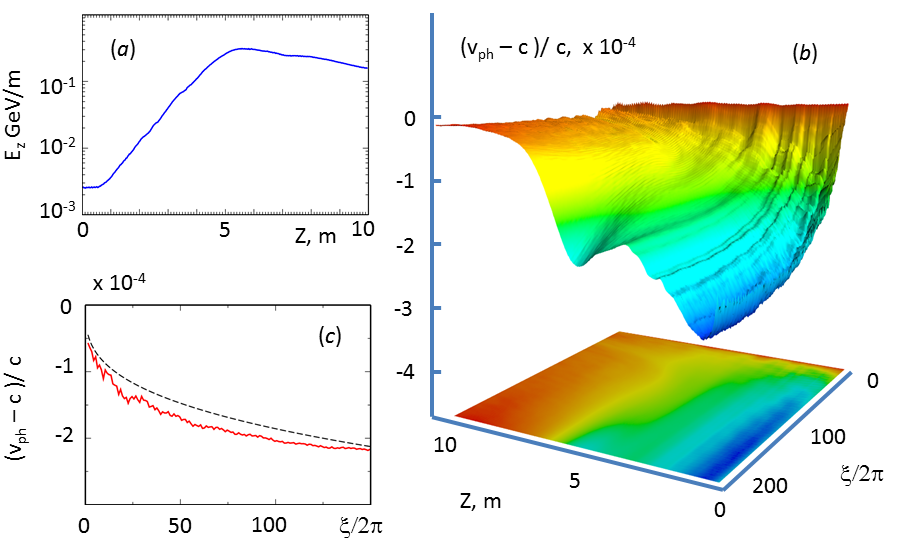
Figure 1: (color online) A 3D hybrid PIC simulation of SPS bunch self-modulation in plasma with constant density $n_{e}=7.76\cdot 10^{14}$ cm^-3. Frame (a) shows the evolution of the maximum accelerating field. The linear instability persists for some 5 meters before the nonlinear saturation. Frame (b) shows the phase velocity of the wake as a surface dependent on the propagation distance $z$ and the bunch coordinate $\xi$. The phase velocity experiences a deep drop towards the tail of the bunch at the linear stage of the instability. When the bunch is completely modulated and the instability saturates at $z>5$m, the wake phase velocity surges up to that of the driving bunch. Frame (c) gives a snapshot of the wake phase velocity after 2.5 meters of propagation distance (the solid red line). The broken line gives the analytical expression (8).

The simulation results are presented in Fig. 1. From the frame (a) we see that the linear instability stage lasts during the first 5 meters of propagation. Then, the bunch is completely modulated and the nonlinear saturation is reached. The wake phase velocity is shown in the frame (b). A significant slowdown of the wake is observed during the instability and along the bunch. The lowest phase velocity is The lowest relative phase velocity is ($\upsilon_{\mathrm{ph}}-c)/c\approx-3.5\cdot 10^{-4}$, corresponding to a wake $\gamma_{ph}\approx 38$. This is an order of magnitude lower than the $\gamma-$factor of the driving bunch. Frame (c) compares the simulation result (the solid red curve) with the analytic expression (8), in which we substituted the SPS bunch parameters. This snapshot of the wake phase velocity has been taken at $z=2.5\,$m, in the middle of the linear instability stage. A reasonable agreement between the simulation and the analytical theory is observed.

The wake slowdown has a dramatic impact on the electron trapping and acceleration. First, it allows for trapping of low energy electrons whose velocities are comparable with the wake velocity. However, the energy gain in the slow wake is very limited due to fast dephasing. The energy gain is given by $\Delta W\approx 4\gamma_{ph}^{2}mc^{2}(E_{max}/E_{WB})$ esarey review . At the linear stage we have $E_{max}\ll E_{WB}$ and the energy gain is low for small $\gamma_{ph}$. The dephasing, however, has a much worse effect : if the electrons have been injected into the early instability phase of the slow wake, they can be lost when they overtake the wave and enter its defocusing phase. The dephasing distance is $k_{p}L_{d}\approx 2\pi\gamma_{ph}^{2}$ and for the slow wake field it can be shorter than the distance needed for the instability to develop. For this reason, the electrons must be injected late in the development of the instability, when the phase velocity begins to grow. In our simulation, the optimum point for injection is located around $z=5\,$m. The wake phase velocity is still low here, but starts growing rapidly as the bunch reaches complete modulation.

A possibility to inject electrons into the wake is side injection side injection . In this case, a bunch of electrons is propagating at a small angle with respect to the driver. The advantage of side injection over on-axis injection is that electrons are gradually “sucked-in” at the right phase by the wake transverse field. This leads to high quality quasi-monoenergetic acceleration of electrons.

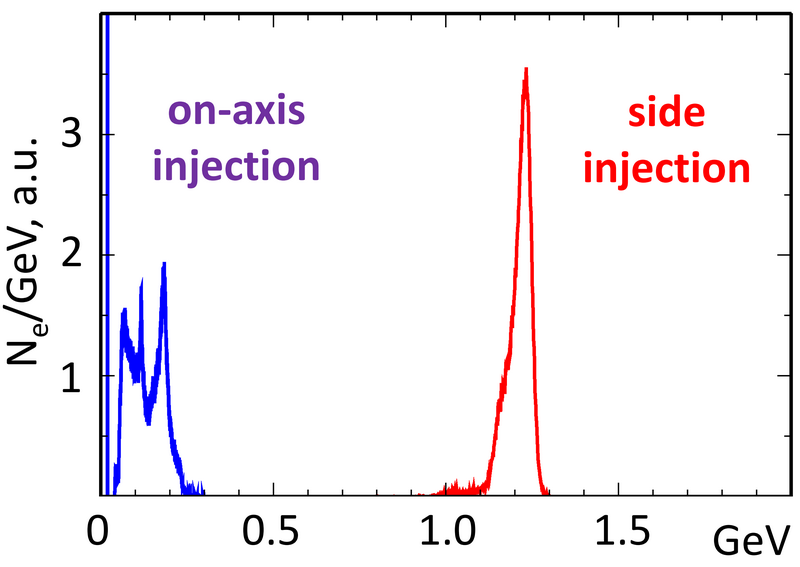
Figure 2: (color online) Electron energy spectra at $z=10\,$m. There were two groups of electrons. One was injected on-axis at the plasma entrance; another was side-injected at the angle of 0.005 radian. In the latter case, the electron bunch trajectory should cross the driver axis at $z=6\,$m, $\xi=20\,$cm behind the bunch head. The on-axis injection lead to a broad spectrum and low energy gain. The side injection resulted in a quasi-monoenergetic beam at 1.2 GeV energy and about 1% energy spread. Initial electron energy was 20 MeV for on-axis injection and 10 MeV for side injection.

In our simulation, we have injected two bunches of test electrons. The first bunch of 20 MeV electrons was injected on-axis at the plasma entrance. This electron energy roughly corresponded to the minimum wake phase velocity at the tail of the driver. We found that during the linearly growing instability stage, these electrons underwent more than one oscillation in the ponderomotive bucket. Finally, after 10 meters of propagation, the maximum energy gain was about 200 MeV with a rather broad energy spectrum as seen in Fig. 2.

The second electron beam with 10 MeV energy was side-injected at an angle of 0.005 radian. The electron bunch trajectory was designed to cross the driver axis at $z=6\,$m, $\xi=20\,$cm behind the bunch head. Due to the small injection angle, however, the electrons were sucked in into the wake much earlier, at the position $z\approx 5$m. The wake transverse fields have put most of the bunch electrons into the focusing and accelerating phase. The electron beam and field configuration just after the electrons entered the wake is shown in Fig. 3. The electron beam is split into micro-bunches located exactly in the accelerating and focusing phases of the wake. Due to this configuration, the side injected beam resulted in a maximum energy gain of 1.2 GeV and a rather narrow energy spectrum.

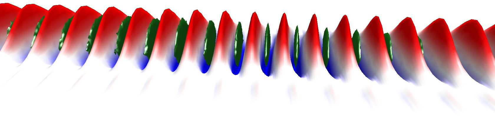
Figure 3: (color online) Test electron bunch (dark green discs) and the accelerating field (the red-blue wave) at $z=5\,$m. The electrons are captured and split into micro bunches located exactly in the accelerating and focusing phases of the wake.

The low energy spread and efficient acceleration of the side injected electrons are also due to the fast rise in the wake phase velocity just after the injection position, as seen in Fig. 1(b). The electrons gain energy while staying in the accelerating phase of the wake.

We have seen above that the growing mode (5) has the low phase velocity (8). There is a way, however, to manage the phase velocity of the wake by employing a gentle longitudinal plasma density gradient as it was discussed in pukhov kostyukov . To elucidate the effect, we have performed an additional simulation with the same beam parameters, but introducing a positive plasma density gradient: $n_{e}(z)=n_{e0}(1+z/d)$ with the characteristic length $d=200$m. The phase velocity obtained in this simulation is shown in Fig. 4.

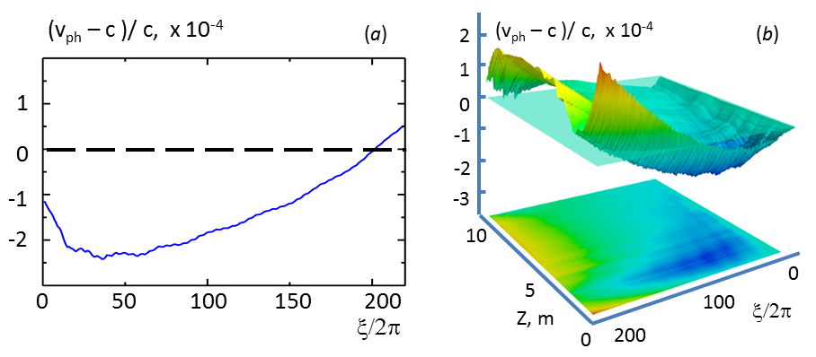
Figure 4: (color online) Phase velocity control by positive plasma density gradient. a) Phase velocity at z=2.5 m. b) Full dynamics picture; the transparent plane marks the speed of light.

The phase velocity at the head of the beam takes a dive as defined by the growing mode dispersion. However, the positive plasma density gradient compensates for the mode dispersion and at the tail of the beam the wake phase velocity becomes equal to the speed of light and even superluminous.

In summary, we have shown that the self-modulational instability of a charged beam in plasma corresponds to a growing mode with a slow phase velocity. The wake velocity is much lower than that of the driver. The wake slowdown is due to the real part of the frequency of the unstable mode. Although this effect limits electron energy gain at the stage of the linear instability growth, the low phase velocity can be harnessed to inject low energy electrons into the wake of a highly relativistic driver. We also have shown that the side injection of electrons at a small angle with respect to the driver axis may drastically improve the quality of acceleration. The transverse field of the wake sucks in the injected electrons and automatically puts them into the right acceleration phase. Finally, we show that the wake phase velocity can be controlled by a longitudinal plasma density gradient.

This work was supported by DFG. V.K., C. S., and G. S. acknowledge funding support from the US Department of Energy under the grant DE-FG02-04ER41321.

References

- (1) T. Tajima and J. M. Dawson, Laser Electron Accelerator, Phys. Rev. Lett. 43, 267–270 (1979).
- (2) Chan Joshi and Victor Malka "Focus on Laser- and Beam-Driven Plasma Accelerators". New Journal of Physics. (2010); C. Joshi et al., Phys. Plasmas 9, 1845–1855 (2002).
- (3) ] C. Joshi, "Plasma Accelerators," Scientific American (February 2006), 294, 40-47
- (4) K. L. Bane, P. Chen, and P. B. Wilson, IEEE Trans. Nucl. Sci. 32, 3524 (1985).
- (5) ] A. Caldwell, K. Lotov, A. Pukhov, and F. Simon, Nat Phys, 5, 363 (2009);
- (6) K.V.Lotov Phys. Rev. ST-AB, 13 041301 (2010).
- (7) E. Esarey, J. Krall, and P. Sprangle, Phys. Rev. Lett., 72, 2887 (1994).
- (8) A. Pukhov and J. Meyer-ter Vehn, Applied Physics B: Lasers and Optics, 74, 355 (2002).
- (9) N. Kumar, A. Pukhov, K. Lotov. Phys. Rev. Lett. 104, 255003 (2010).
- (10) E. Esarey, et al. Rev. Mod. Phys. 81, 1229 (2009).
- (11) N. E. Andreev et al., IEEE TPS 24, 363 (1996).
- (12) A. Bers, “Basic plasma physics 1,” (North-Holland Publishing Company, 1983) Chap. 3.2.
- (13) K.V.Lotov, Phys. Plasmas {\bf 18} 024501 (2011).
- (14) T. Tueckmantel et al, IEEE TPS 38, 2383 (2010).
- (15) S. Yu. Kalmykov et al., Phys. Plasmas 13, 113102 (2006).
- (16) A. Pukhov, I. Kostyukov, Phys. Rev. E 77, 025401 (2008).
- (17) D. Whittum et. al., Phys. Rev. Lett. 67, 991 (1991).