Bubble collisions and measures of the multiverse
Abstract:
To compute the spectrum of bubble collisions seen by an observer in an eternally-inflating multiverse, one must choose a measure over the diverging spacetime volume, including choosing an “initial” hypersurface below which there are no bubble nucleations. Previous calculations focused on the case where the initial hypersurface is pushed arbitrarily deep into the past. Interestingly, the observed spectrum depends on the orientation of the initial hypersurface, however one’s ability observe the effect rapidly decreases with the ratio of inflationary Hubble rates inside and outside one’s bubble. We investigate whether this conclusion might be avoided under more general circumstances, including placing the observer’s bubble near the initial hypersurface. We find that it is not. As a point of reference, a substantial appendix reviews relevant aspects of the measure problem of eternal inflation.
1 Introduction
String theory argues for the existence of an enormous landscape of classically-stable, positive-energy vacua (in addition to other states) [1, 2, 3]. The semi-classical methods of Coleman and De Luccia (CDL) indicate that such vacua can decay via bubble nucleation, the internal bubble geometry described by an open Friedmann–Robertson–Walker (FRW) metric, with decay rates (per unit volume) that are generically exponentially suppressed [4, 5, 6]. Meanwhile, in sufficiently long-lived, positive-energy vacua, spacetime expands at a rate faster than it succumbs to decay, hence the volume grows without bound [7, 8]. Thus emerges a picture of spacetime in which our local Hubble volume is merely part of the inside of an open-FRW bubble, which (likely) nucleated in some other bubble, and so on; where in each positive-energy bubble other bubbles endlessly nucleate and sometimes collide [9].
Although in this picture our local Hubble volume resides entirely within one such bubble, collisions between our bubble and others are potentially observable, if they occur within our past lightcone. The probability distribution of observable bubble collisions was first estimated by Garriga, Guth, and Vilenkin (GGV) [10]. The calculation involves choosing a measure over the diverging spacetime volume of potential bubble-nucleation sites, including choosing an “initial” hypersurface below which there are no bubble nucleations. Motivated in part by the expectation of exponentially-suppressed transition rates, GGV took the initial hypersurface to correspond to a constant-time slice in the infinite past (in a spatially-flat de Sitter chart). Remarkably, the spatial distribution of bubble collisions across an observer’s sky features an anisotropy, indicating the orientation of the initial hypersurface, despite its relegation to the infinite past, a phenomenon dubbed “persistence of memory.”
Freivogel, Kleban, Nicolis, and Sigurdson (FKNS) later studied the same question in what is expected to be a more realistic cosmology, in which the energy density of the vacuum in which our bubble nucleates—the “parent” vacuum—is much greater than that of the inflationary epoch within our bubble [11]. In this case the effects of the initial hypersurface are heavily suppressed, in particular the spatial distribution of bubble collisions becomes isotropic except over a solid angle that is too small to reasonably expect enough bubble collisions there to reveal the anisotropy. Thus, the relatively small (inflationary) vacuum energy of our bubble effectively screens this information about initial conditions.
While it is reasonable to push the initial hypersurface to past infinity, it is worthwhile to consider what might be the signatures of other possibilities. In particular, one might speculate that if our bubble nucleates not far from the initial hypersurface, then the orientation of the hypersurface might leave some mark in the spatial distribution of bubble collisions in our sky. As a point of motivation, one might imagine that semi-classical spacetime emerges from some more quantum state via what appears within the semi-classical spacetime to be a “tunneling from nothing” transition [12], with an “initial,” near-Planck scale vacuum rapidly decaying in a cascade of CDL bubble nucleations, one of which is our bubble. An immediate objection to this picture is that CDL transition rates are proportional to , where is the Euclidean action of the instanton minus that of the background (in Planck units), and in the semi-classical limit where the analysis can be trusted should be very large. However, it is possible that semi-classical methods give a qualitative description of the geometry even at near-Planck scales, in which case transition rates may frequently be only weakly suppressed. Another reason one might be skeptical of this possibility is that it assumes we live among first wave of bubble nucleations, as opposed to among the diverging number of bubbles that nucleate far from the initial hypersurface (in the global spacetime, assuming eternal inflation). Yet, some phenomenologically viable measures weigh events in spacetime according to their occurrence within the vicinity of a single worldline originating in the initial vacuum (surveying all semi-classical future histories of the worldline). In this case our residence in one of the early bubbles is not necessarily very surprising, since the probability of residing in a given bubble is suppressed by the branching ratio implied by the series of transitions required to reach it from along a worldline originating in the initial vacuum.
In light of possibilities like this, we study the spatial distribution of bubble collisions in an observer’s sky, while remaining open to the possibility that our bubble resides near the initial hypersurface below which there are no bubble nucleations, and being mindful of other considerations raised by choosing a measure over the diverging volume of eternal inflation. (We include a partial review of the measure problem, insofar as it pertains to the issue of bubble collisions, in the appendix.) We focus on two basic choices for the initial hypersurface, (1) the minimal spacelike Cauchy surface in the closed de Sitter chart (which can be seen as the surface defining initial conditions in the wake of a tunneling-from-nothing event), and (2) the null cone representing the past-directed boundary of an open de Sitter chart (which can seen to approximate the bubble wall of the parent vacuum). Either of these will look like the GGV choice of initial hypersurface in the limit where the hypersurface is pushed in the deep past. The effect of the measure is to prescribe at what global time coordinates bubbles like ours typically nucleate (the focus of this paper being times on order of the Hubble rate in the initial vacuum) and at what FRW radial coordinate observers typically arise.
We find that the FKNS prediction of an isotropic distribution of bubble collisions is robust with respect to all of these considerations; the only scenario in which the distribution is anisotropic over an appreciable fraction of the observer’s sky is when the vacuum energy density of the parent vacuum is not much larger than the inflationary energy density in our bubble, in which case the likelihood to observe a significant number of bubble collisions appears to be small. (We assume the relevant portion of the multiverse has 3+1 large spacetime dimensions. Significant anisotropy in the distribution of bubble collisions can result if the parent vacuum has fewer than three large spatial dimensions, as in [13].)
This work benefits from techniques largely developed elsewhere [14, 15, 16, 17, 18, 19], including the references above. Although we do not discuss any specific observational signatures of bubble collisions—focusing instead on the potential to observe such effects by studying the overlap of causal domains—there is a growing body of literature exploring these signals [20, 21, 22]. Indeed, [23, 24] have developed a search algorithm for some of these effects in the cosmic microwave background data, indicating features consistent with (but not demonstrative of) bubble collisions. For a recent review of these and other topics, see [25].
The remainder of this paper is organized as follows. We establish the geometry under consideration in Section 2; the main deviation from previous work occurs in Section 2.2, where we describe our choices for the initial hypersurface. The distribution of (potentially) observable bubble collisions is calculated in Section 3. In Section 4, we perform a quick study of the impact of other bubble collisions in our past lightcone. Concluding remarks are given in Section 5. The appendix provides a partial review of the measure problem of eternal inflation, with the focus on issues relevant to the study of bubble collisions.
2 Geometry
We consider cosmologies in which our local Hubble volume is contained within an open FRW bubble, “our bubble,” which formed via CDL barrier penetration in a landscape of metastable vacua. The progenitor of our bubble, the “parent” vacuum in which our bubble nucleates, has positive vacuum energy density, so as to permit such a transition. We take the bubble walls to be thin and approximate their trajectories as following null cones emanating from the centers of essentially point-like bubble nucleations. Roughly speaking, these approximations are valid when the tension of the bubble wall is small compared to the energy difference between the vacua, in units of the curvature radius of the parent vacuum [4]. Outside the context of a specific model of the landscape, it is unclear how easily this condition is made consistent with rapid bubble nucleation rates. Therefore, our calculations should be interpreted as providing only qualitative insight. We everywhere work in 3+1 spacetime dimensions.
2.1 Coordinate systems
Among the consequences of the above approximations is the geometry of the parent vacuum is subset of de Sitter (dS) space. We make use of the closed dS chart, with the line element
| (1) |
where and . Here and below gives the line element on the unit two-sphere, and denotes the dS curvature radius. It is convenient to refer to an embedding of the geometry in (4+1)-dimensional Minkowksi space, with
| (2) |
dS space (with curvature radius ) is then the geometry induced on the hyperboloid
| (3) |
The closed dS chart covers the entire hyperboloid, as indicated by the embedding
| (4) | |||||
| (5) | |||||
| (6) | |||||
| (7) | |||||
| (8) |
We also make use of the spatially-flat dS chart, with the line element
| (9) |
where and . This covers only half of the full dS hyperboloid (corresponding to ), as can be seen from the embedding in Minkowski space,
| (10) | |||||
| (11) | |||||
| (12) | |||||
| (13) | |||||
| (14) |
The embedding space makes clear how to transform between the charts. Coordinates on the unit two-spheres can be matched trivially. The remaining coordinates are then related by
| (15) |
Let us now consider our bubble. The discussion is simpler if we first imagine that the geometry of our bubble is also a subset of the dS geometry, with curvature radius (with ). The corresponding hyperboloid in the embedding space can be shifted in the direction, so as to allow for a continuous (though not smooth) matching between it and the parent-vacuum hyperboloid, at what will be understood as the bubble wall. In particular, we momentarily consider the bubble geometry to be that induced on the hyperboloid
| (16) |
It can be seen that the two hyperboloids intersect on the plane . This corresponds to bubble nucleation at , i.e. in the closed dS chart (we often suppress the coordinates on the unit two-sphere). Per our assumption of negligible initial bubble radius, the bubble wall is defined by (i.e. the intersection of the future lightcone of the point of nucleation and the hyperboloid), which gives
| (17) |
Of course, we are interested in bubbles featuring an inflationary and big-bang cosmology consistent with our observations, as opposed to the empty dS space on (16). The geometry of such bubbles can be covered with open FRW coordinates, with the line element
| (18) |
where (given positive vacuum energy in our bubble) and . It is often convenient to refer to the conformal time in the bubble, defined by
| (19) |
The time dependence of the scale factor , and likewise the maximum time , depends on the matter content of the bubble. We adopt a simple approximation of the standard inflationary plus big-bang cosmology, the details of which are described as they become relevant below. It is possible to embed this generic open FRW geometry in the higher-dimensional Minkowski space. With some hindsight regarding the appearance of , we write
| (20) | |||||
| (21) | |||||
| (22) | |||||
| (23) | |||||
| (24) |
where the function corresponds to a solution of the differential equation
| (25) |
dots here denoting derivatives with respect to .
Although the CDL instanton generates a homogeneous and isotropic FRW bubble, it is necessary for there to be a round of slow-roll inflation within the bubble. This is to redshift away the large initial spatial curvature of the bubble, so as to agree with our observation of an approximately flat FRW geometry. For simplicity, we treat the inflaton energy density as equivalent to vacuum energy density, taking . Furthermore we assume nothing else contributes significantly toward the energy density of the bubble, until reheating. The scale-factor solution before reheating is then
| (26) |
which incorporates the appropriate CDL boundary conditions. We have set an integration constant so that proper and conformal time in the bubble are related during inflation by
| (27) |
This scale-factor solution corresponds to the open dS chart, and is embedded into the higher-dimensional Minkowski space by inserting it into (20)–(24), with . This inflationary geometry therefore coincides with the dS geometry induced on the hyperboloid (16), and therefore matches continuously onto the parent vacuum geometry at the bubble wall. Of course, the geometry of the bubble after reheating is no longer locally dS space, and will therefore deviate from the dS hyperboloid.
2.2 The initial hypersurface
Our cosmological setup involves an initial hypersurface, below which we presume there are effectively no bubble nucleations. We consider two possibilities, which are most easily described starting with pure dS space (i.e. without any bubble nucleations). Then, the hypersurface could correspond to the surface of initial conditions in a “tunneling from nothing” scenario [12], while the hypersurface could correspond to what might roughly appear like an initial hypersurface if for example the bubble wall of the parent vacuum is such that it screens the effects of all bubble nucleations outside of it. For brevity we henceforth refer to these as the “tunneling from nothing” and “bubble wall” initial hypersurfaces.
These hypersurfaces break a dS symmetry, a consequence of which is we cannot place the nucleation of our bubble at without loss of generality. (The remaining dS symmetries still allow us to place the nucleation of our bubble at .) Instead, our bubble generically nucleates at some point , . Note however that the point can be translated to the point by performing a boost in the embedding Minkowski space; in particular by taking
| (28) | |||||
| (29) |
where , , and are unchanged, and where with
| (30) |
Here is the proper time between and , keeping all other coordinates fixed at the origin. Thus, we have the option of working with the initial hypersurfaces or , with our bubble nucleating at , or working with the boosted initial hypersurfaces (see below), with our bubble nucleating at . We choose the latter.
The would-be initial hypersurface corresponds to what would have been the plane in the embedding coordinates. Boosting this hypersurface so as to translate our bubble to the origin, we have , which corresponds to
| (31) |
Meanwhile, the would-be hypersurface corresponds to what would have been the plane in the embedding coordinates. Boosting this hypersurface so as to translate our bubble to the origin, we have , which corresponds to
| (32) |
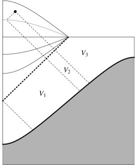
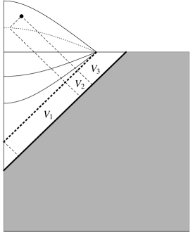
Two toy conformal diagrams of the bubble plus parent vacuum geometry, including the boosted initial hypersurfaces, are displayed in Figure 1.
 |
 |
It is convenient to perform another boost, so as to translate an observer in our bubble from the random position , to the more central position position . (Rotational invariance has allowed us to set without loss of generality. Although unbroken FRW and dS symmetries would also allow us to set , we have already exploited the corresponding symmetry to set .) In light of the embedding (20)–(24), we see this can be accomplished (for arbitrary scale-factor ) with the boost
| (33) | |||||
| (34) |
keeping , , and fixed, where with
| (35) |
Note that this boost leaves intact the trajectory of the bubble wall: in terms of the embedding coordinates, we have .
Aside from translating the observer to the “center” of our bubble, the effect of the above boost is to perform a second rotation on the initial hypersurface. For the initial hypersurface of (31), we have , or
| (36) |
This describes the embedding of the “tunneling from nothing” initial hypersurface as seen by an observer in our bubble who places herself at . For the initial hypersurface (32), we have , which corresponds to
| (37) |
This describes the embedding of the “bubble wall” initial hypersurface as seen by the above-mentioned observer. Note that this boost has introduced -dependence in both initial hypersurfaces. This can be seen in Figure 1 in the following way. Take the toy conformal diagrams there to display the geometry for (). Then we can augment the diagrams with the geometry at () by attaching the mirror image of each diagram to its left. Then it can be seen that the observer, by virtue of residing to the right of the origin, has more of the initial hypersurface in her past lightcone to the right () than to the left ().
The ultimate cause of this anisotropy is the breaking of a background dS symmetry by the choice of initial hypersurface, and it is the root of the “persistence of memory” effect mentioned in a slightly different context in the introduction. In particular, if we take the late-nucleation-time limit (corresponding to and ), we find both initial hypersurfaces (36) and (37) become
| (38) |
which corresponds to the GGV surface mentioned in the introduction.
2.3 Matching coordinates inside and outside the bubble
Our calculations require us to map null rays from the parent vacuum into our bubble. We are only interested in incoming, radial null rays, and we match them by identifying coordinates at the bubble wall, using the Minkowski embedding space described in Section 2.1. In terms of the closed dS chart of the parent vacuum, we can label a given null ray according to the coordinates at which it originates, its trajectory given by . In this chart the bubble wall corresponds to , and so according to the embedding (4) we have at the bubble wall. In the open dS chart of our bubble, the bubble wall corresponds to and , with held constant, and so according to the embedding (20) with the scale-factor solution (26) we have . Performing the matching, we find its trajectory in terms of the FRW bubble coordinates to be
| (39) |
For later reference we also construct a mapping between certain geodesics in the parent vacuum and their extensions into our bubble. The calculation is a bit technical, and benefits from reference to [26, 27] (see [28, 29] for more background). Again, we make use of the Minkowski embedding space, and suppress the unit two-sphere by defining
| (40) |
Our approach takes advantage of the fact that geodesics in dS correspond to the intersection of the dS hyperboloid and plane hypersurfaces that pass through the origin of the hyperboloid, in the embedding geometry.111The author thanks Daniel Harlow and Leonard Susskind for pointing this out. For geodesics in the parent vacuum, we write the plane
| (41) |
For example, a geodesic with constant radial coordinate in the spatially-flat dS chart has , as can be seen via the embedding (10)–(14). A geodesic with constant radial coordinate in the closed dS chart has , , c.f. (4)–(8). We can use (29) to boost this plane so as to describe a geodesic that is orthogonal to the initial hypersurface (36); this gives and .
Since we approximate the inflationary phase within our bubble as pure vacuum-energy domination, geodesics in the inflating spacetime can also be described as the intersection of a plane hypersurface and a dS hyperboloid. In this case we write the plane
| (42) |
where accounts for the translated origin of the dS hyperboloid describing the inflationary epoch within our bubble, (16). In order for this geodesic to describe the extension of the parent-vacuum geodesic given by (41), the plane (42) should intersect (41) at the bubble wall (given by ), and the tangents to the geodesics should each make the same angle with the tangent to the bubble wall (at the point of intersection). Solving for and in terms of and in this way provides a map between geodesics in the parent vacuum and geodesics in the inflating region of the bubble. Since during inflation in the bubble geodesics rapidly asymptote to comoving in the bubble FRW frame, this serves as a map between geodesics in the parent vacuum and comoving geodesics in the bubble.
The algebra is a bit messy, so we only lay it out symbolically. Combining (41) with the hyperboloid constraint (3), we can solve for the components and of the geodesic as a function of . We thus write the geodesic as a curve in the embedding space,
| (43) |
where the index is understood to run over the three components of the vector. Likewise, combining (42) with (16), we obtain the curve . The curve describing the bubble wall is simply . Using this we can compute the (Minkowski) times at which the curves and intersect the bubble wall. These are, respectively
| (44) |
We denote the tangents to and with and , respectively. For example,
| (45) |
where is an infinitesimal proper time interval, , with denoting the Minkowski metric on the embedding space with the unit two-sphere suppressed. For the tangent to the bubble wall we can simply take . As described above, we solve for and in terms of and by solving
| (46) |
where all expressions are evaluated at the bubble wall, i.e. at (44). The solution is
| (47) |
The inflationary geometry within the bubble is embedded by using (20)–(24) with the scale-factor solution (26). Inserting this into (42), one can solve for the radial coordinate of the geodesic in terms of and , in the limit . This gives
| (48) |
For a geodesic that is initially comoving at radial coordinate with respect to the spatially-flat dS chart, combining this with (47) and the results below (41) gives
| (49) |
For a geodesic that is orthogonal to the initial hypersurface (36) in the closed dS chart,
| (50) |
Although the above matching has been performed only with respect to the inflationary geometry within the bubble, the dS coordinate matches trivially onto the post-inflationary open-FRW coordinate denoted by the same symbol.
Finally, for later reference we also compute the scale-factor time between some reference hypersurface—here taken to be the surface of fixed time in the spatially-flat dS chart—and a fixed FRW time hypersurface in the bubble. Consider a congruence of initially constant- geodesics that enter our bubble and become comoving along the set of radial coordinates , according to (49). Note that, tracing along these geodesics, a small coordinate separation at evolves into a comoving coordinate separation
| (51) |
at . Thus, a radial comoving rod covering physical distance at covers a physical distance at . Moreover, a comoving “annulus” centered at with physical three-volume at covers an annulus centered at with physical three-volume at . Defining the scale-factor time to be one third the logarithm of the implied expansion factor, we see
| (52) |
where we have exploited the symmetry of the annulus to equate the change in logarithm of its volume expansion factor with the change in logarithm of the local volume expansion factor.
2.4 Bubble collision geometry
With the parent vacuum and our bubble in place, we now introduce an additional bubble, the colliding bubble, the effects of which we hope to observe. The collision between the colliding bubble and our bubble occurs along the bubble walls, but in our approximation of point-like bubble nucleation with thin bubble walls, this corresponds to at the intersection of the future lightcones of the bubble nucleation events. We focus on the possibility that the bubble collision leaves some imprint on the cosmic microwave background—small enough to have so far evaded unambiguous detection, but not so small so as to be undetectable—in which case we are interested in the intersection of the past lightcone of the observer, the hypersurface of recombination, and the future lightcone of the colliding bubble nucleation event.
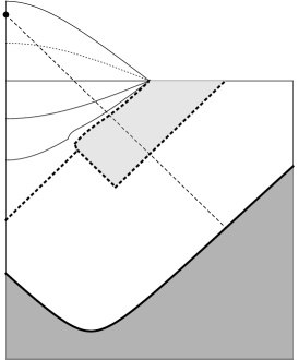
Although our analysis avoids reference to the microphysics of the collision, it might help to draw a more concrete picture. Consider a landscape effectively described by some number of scalar fields, the metastable states in the landscape corresponding to local minima in the scalar-field potential. Bubble nucleations occur via CDL barrier penetration, but in vacua like ours the instanton itself does not take the tunneling field all the way to the local minimum; instead it arrives at rest on the other side of the potential barrier, drives slow-roll inflation as it classically evolves down a shallow slope in the potential, and reheats the bubble as the field finally oscillates around the local minimum. When our bubble collides with another one, a domain wall forms between our vacuum and another one (the other vacuum is not necessarily that of the colliding bubble [30, 31]). This domain wall moves away from the center of our bubble, unless the vacuum energy behind the domain wall is smaller than ours, in which case the tension of the domain wall is important for determining its trajectory [14]. In the first case, the domain wall does not follow precisely what would have been the trajectory of the bubble wall in the absence of a collision, and so the domain wall can perturb the initial value of the inflaton field in the bubble. (The left panel of Figure 2 provides a cartoon illustration.) This perturbation might be large, but it is redshifted during inflation, and if inflation does not last too long (not more than roughly ten -folds more than is necessary to solve the flatness problem), it might produce small but observable signatures [20, 21, 22].
 |
 |
On the other hand, if the aforementioned domain wall moves toward the center of our bubble, it significantly disrupts the FRW geometry in its wake. (The right panel of Figure 2 provides a cartoon illustration.) In regions within our bubble where inflation proceeds more or less as before, we have the same story as above. In regions where inflation is significantly disrupted (including regions in the colliding bubble vacuum on the other side of the domain wall), it is reasonable to expect that observers like us who reside in large galaxies do not arise to observe the effects. At this point, we must simply assume that most of the volume within our bubble (after regulating the diverging volume with a spacetime measure, see the appendix) falls into one of these categories, so that it is not unusual for observers like us to observe a (nearly) flat FRW Hubble volume as we do.
Proceeding now with our analysis, we denote the location of the point of nucleation of the colliding bubble , where we have used the remaining symmetry on the unit two-sphere to place both the observer and the center of the colliding bubble nucleation event at . For notational simplicity we work on a hypersurface of constant and suppress the dependence on ; in the end the complete results are easily obtained by utilizing the rotational symmetry of the problem.
It is complicated to work out the coordinates of the future lightcone of the colliding bubble nucleation event, let alone transform and evolve them in terms of our bubble coordinates. Instead we approximate the relevant portion of the lightcone—that is, the portion that will intersect the past lightcone of the observer and the surface of last scattering—as a constant “front” (following [11]). That is, we start with the future lightcone in the plane,
| (53) |
Using (39), we match the null ray onto the open FRW coordinates of our bubble, giving
| (54) |
The observable portion of the future lightcone of the colliding bubble nucleation event is then approximated as a plane orthogonal to this trajectory, i.e.
| (55) |
The above approximation is accurate because the intrinsic curvature on the hypersurface corresponding to the future lightcone of the colliding bubble, after propagation into our bubble, is of order the curvature radius of our bubble, which is empirically much larger than the distance to (and across) the surface of last scattering.
In Section 2.2 we performed a boost in the Minkowski embedding geometry, so as to place an arbitrary observer in the bubble at . The surface of last scattering for this observer then corresponds to the two-sphere with radial coordinate , on the hypersurface , where is the FRW (conformal) time of the observer and is the time at recombination. The intersection of the surface of last scattering and the future lightcone of the colliding bubble nucleation event then corresponds to the region . Thus, the effects of the bubble collision are limited to
| (56) |
Let us discuss the meaning of (56). When , the collision occurs too late for its future lightcone to intersect the surface of last scattering. These bubble collisions are unobservable by virtue of causality. They correspond to bubble nucleations in the region marked in Figure 1 (note that Figure 1 displays the geometry before the boost that takes ). When , the collision occurs so early that its future lightcone covers the entire cosmic microwave sky of the observer. These bubble collisions are in principle observable, but the redshifting of their features during inflation combined with the lack of contrast with an unaffected region on the cosmic microwave background would seem to make them undetectable. They correspond to bubble nucleations in the volume marked in Figure 1. Only bubble nucleations in the volume marked in Figure 1 intersect the surface of last scattering so as give a real, non-zero solution for in (56), corresponding to the angular scale of the collision region on the observer’s sky. We consider only these bubble collisions potentially observable.
Before proceeding, for future reference we compute the solid angle subtended by the intersection of our bubble wall and the colliding bubble wall, as a function of time. That is, at any given time the bubble wall of our bubble is a two-sphere, as is the bubble wall of any colliding bubble, and we compute the solid angle of the intersection of these two two-spheres, from the perspective of within our bubble. As always we suppress the coordinate, and for simplicity we take the colliding bubble to nucleate at (symmetry guarantees that the final result is independent of ). It is easiest to work in terms of the Minkowski embedding coordinates. Then the future lightcone of the colliding bubble corresponds to the intersection of the future lightcone of its nucleation point,
| (57) |
and the dS hyperboloid of the parent vacuum, (3). We have used the embedding (4)–(8) to convert the colliding bubble nucleation point into embedding coordinates. The future lightcone of our bubble is simply . It is straightforward to solve this system of equations for the angle of their intersection, which gives
| (58) |
as a function of the closed dS chart time along the intersection.
3 Distribution of observable bubble collisions
To compute the spatial distribution of bubble collisions on an observer’s sky, we integrate over the spacetime volume available for colliding bubble nucleations, as a function of the coordinates on the unit two-sphere parametrizing the observer’s sky. The differential number of bubbles nucleating as a function of the closed dS coordinates can be approximated
| (59) |
where is the bubble nucleation rate per unit four-volume . This is only an approximation because it treats the four-volume in the future lightcone of any bubble nucleation event the same as the four-volume of the parent vacuum, when in fact the geometry and the bubble nucleation rate will in general be different there. We return to this issue in Section 4.
The available volume for colliding bubble nucleations naturally divides into three sectors, labeled , , and in Figure 1. As described in Section 2.4, in this work we consider only colliding bubble nucleations in region to be observable. Thus, we are interested in the spatial distribution of bubble collisions coming from there. The corresponding volume is bounded in part by our bubble wall, which is approximated as the future lightcone of the center of our bubble nucleation event. This gives the constraint
| (60) |
The region is additionally bound by the requirement that (56) has a real solution for the coordinate on the observer’s sky; this gives the constraints
| (61) |
Finally, is bounded by the initial hypersurface below which we presume there are no bubble nucleations. According to our assumptions, this is given by either (36) or (37).

These constraints suggest a new set of coordinates, , where
| (62) |
Hypersurfaces of constant or constant are lightsheets, with corresponding to the past lightcone of our bubble nucleation event, and corresponding to its future lightcone, as indicated in Figure 3. We take to run from minus one to one, so that the (suppressed) coordinate runs from zero to . The region corresponds to intervals
| (63) | |||||
| (64) |
where we have used . In the case of the initial hypersurface (36), is given by
| (65) |
while in the case of the initial hypersurface (37), it is given by
| (66) |
The parameters , , , and are determined by the proper time between the initial hypersurface and our bubble, and the FRW radial coordinate of the observer in our bubble; see Section 2.2. In terms of these coordinates, the differential volume element is given by
| (67) |
3.1 Assumptions about model parameters
Integrating the differential volume element (67) within the regions delineated above is rather complicated. It is therefore convenient to introduce some simplifying approximations. To begin, note that the current observational bound on the spatial curvature, (WMAP+BAO+SN 95% confidence level bound for prior [32]), implies that the comoving distance to the surface of last scattering satisfies . We therefore expand in . Meanwhile, the current observational bound on the amplitude of tensor perturbations on the surface of last scattering implies [32]. While it is not necessary that the parent vacuum have near Planck-scale energy density, this seems like a plausible assumption for typical states in the landscape, and appears to be required to permit the rapid decay rates we consider in this paper. Therefore we also assume .
To further simplify results, it is often assumed that the original FRW radial coordinate of the unboosted observer, , tends to infinity. This is justified as follows. The FRW symmetries of the bubble would seem to make any unit three-volume on a given constant–FRW time hypersurface as likely as any other to contain an observer. At the same time, the hyperbolic geometry of the constant-FRW time hypersurface implies that the three-volume is dominated by regions at large . One would therefore expect a randomly-selected observer to reside at large , with in the limit of considering the entire bubble geometry. However, these assumptions are problematic on multiple levels. The result itself points to an unregulated divergence, stemming from the diverging volume in the bubble. Regulating this divergence requires introducing a measure over the diverging volume of eternal inflation. As it stands, it is unclear what the “correct” spacetime measure is, and different seemingly natural choices give very different cosmological predictions. In the appendix we provide a detailed, if partial, review of the measure problem of eternal inflation.
At present, there is no viable measure that assigns equal likelihood (on average) for an observer to arise in any unit three-volume on a constant-FRW time hypersurface in the bubble, and is at the same time sufficiently precisely defined so as to predict, for example, the spatial distribution of bubble collisions on an observer’s sky. Measures that have been understood to provide such a prediction have been found to suffer from Boltzmann brain domination and runaway inflation (see the appendix). Moreover, it must be acknowledged that while the FRW symmetries that motivate such an approach hold to good approximation in some regions within a given bubble, they do not constitute a set of global symmetries on which a measure can be constructed, because of the effects of bubble collisions.
The various measure proposals described in the appendix all point toward the same qualitative prediction: observers like us typically reside at , with the distribution falling off exponentially with for greater than one. Therefore, we take and make the corresponding assumption for . We also take and make the corresponding assumption for . Here is the proper time between the nucleation of our bubble and the initial hypersurface (in the comoving frame of the parent vacuum). Note that although we are interested in rapid vacuum decay rates, decays rates that are minuscule next to the Hubble rate of the parent vacuum would preclude the very notion of a metastable parent vacuum. (A more precise statement of the assumption used below is , which might be seen to offer greater leeway toward considering rapid parent-vacuum decay rates.) As a point of reference, note that the transition to eternal false-vacuum inflation occurs when the total decay rate satisfies [8]
| (68) |
where is determined numerically to be . This corresponds to the rough expectation at the transition to eternal inflation.
Finally, consider the cosmology within our bubble. This begins with a period of curvature domination, with the subsequent period of inflation beginning when ; recall the scale-factor solution (26). Empirically, the number of -folds of inflation is large, , meaning that by the end of inflation the FRW conformal time has become very small in magnitude, . It can be shown that during its subsequent evolution, the conformal time becomes positive (since radiation domination lasts for a proper time interval ), but the total change in is dominated by its growth between recombination and the present (since the present FRW proper time is much greater than it was at recombination), during which changes by an amount
| (69) |
Thus, and the present conformal time can be approximated
| (70) |
Because we work in terms of conformal time, and because we are only interested in the potential observability of bubble collisions due to the causal structure of the multiverse, this is the only cosmology in our bubble on which we rely.
3.2 Analysis of the distribution function
It is straightforward to integrate (67) with respect to , and doing so we find
| (71) |
Notice that the result is greatly simplified if we assume and , in accordance with the assumptions about model parameters outlined in Section 3.1 above (we discuss this approximation in greater detail below). Then we find
| (72) |
independent of . The independence of indicates that the spectrum of observable bubble collisions is dominated by collisions with bubbles that nucleate near , i.e. near the bubble wall of our bubble. Likewise, the differential number of bubbles is isotropic with respect to the coordinates on the two-sphere of the observer’s sky.
The integral over is now trivial. Before we report the result, note that there is a simple correspondence between the coordinate and the angular scale of the region affected by the bubble collision on the observer’s sky. Defining the angular scale to be the largest value of affected by the bubble collision, from (56) we see
| (73) |
Thus, , i.e. we obtain the standard result that the distribution of angular scales is uniform in . Returning to (72) and performing the integrations, we obtain
| (74) |
where we have expanded in . This confirms the well-known result, giving hope for observable bubble collisions if and are not too small.
The comoving distance to the surface of last scattering falls off exponentially with the number of -folds of inflation in our bubble, . In light of (74), one might worry that an overwhelming probability for to be significantly larger than the current observational constraint makes the expected number of (observable) bubble collisions far below one. While this is a valid concern, there are reasons to be hopeful. The expected number of -folds of inflation depends on the landscape distribution of and on the measure regulating the diverging spacetime volume of eternal inflation. In the first case, there is cause to expect that a large number of -folds might be difficult to achieve in the string landscape, with the admittedly crude estimation of [33] indicating a distribution that falls off like . Meanwhile, measure proposals that weigh by the inflationary expansion factor in a bubble suffer from runaway inflation in a large landscape, giving cause to exclude them (see the appendix). Indeed, none of the measure proposals described in Section A.2 give a preference for one bubble over another based on it having a larger number of -folds of inflation. Indeed in several cases the distribution of the curvature parameter has been predicted, conditioning on present observational constraints, and in each case one finds a roughly one in ten chance that (corresponding to ) [34, 35, 36].
It is informative to reconsider the inequalities that lead to the result (72). After restricting attention to “observable” bubble collisions, which limits to lie in the interval (63), the inequality follows directly from our assumption . For the moment take this as given, and consider the inequality . In the case of the “tunneling from nothing” initial hypersurface of (36), is given by (65). Then the inequality can only fail if is very near to one. This implies that must be large, and the inequality fails either when or when , depending on whether or not (recall that ). The first possibility actually does not admit a solution for , while the second possibility holds only when falls within a narrow window near minus one (if also ). The number of bubble collisions coming from this angular region in the observer’s sky would be . Even under our assumption of rapid decay rates, it is hard to accept that this number could be large enough to detect a significant deviation from the otherwise isotropic distribution of bubble collisions.
A similar analysis applies to what we have called the “bubble wall” initial hypersurface of (37), for which is given by (66). In particular, assuming as before , the inequality fails only when is very near to one, and even in that case only when lies within a narrow window near minus one. The specifics differ only in the placement of factors of and , and assuming the former isn’t too small (i.e. assuming ), then we reach the same qualitative conclusion: the anisotropy in the spectrum of bubble collisions is limited to an angular region (if also ), from which a negligible number of bubble collisions are available to experimentally resolve the anisotropy.
These arguments fail when is not large, i.e. when . In this case the integration over covers only a small interval , which allows us to approximate the integral by keeping the argument fixed, evaluated at the mean value . This gives
| (75) |
By inspecting (65) and (66), we see that the magnitude of is never much greater than one (given the present hypothesis that is not much greater than one), and at the same time is always positive and is always negative, so (75) does not feature any poles. Thus we come back to the conclusion from above: although now features anisotropy over a broad angular region, the total number of bubble collisions coming from this region is small, and therefore the anisotropy is unobservable. We note that this is the same effect found by FKNS in their study of the GGV “persistence of memory,” in the case where the initial hypersurface is pushed far into the past of our bubble.
The above analysis considers only two orientations of the initial hypersurface. However it seems reasonable to suppose that insofar as the semi-classical multiverse can be described in terms of evolution from an initial hypersurface below which there are no bubble collisions, that such a hypersurface will thread somewhere between the two orientations that we consider, in which case we expect the same results. Thus we conclude that if the effects of a significant number of bubble collisions are observable, the distribution of these collisions on an observer’s sky will appear isotropic, with the angular scale of collision regions distributed uniformly with respect to , regardless of our proximity to any surface specifying initial conditions.
4 “Unobservable” bubble collisions
In studying the distribution of bubble collisions in Section 3, we ignored colliding bubbles coming from the region in Figure 1, because as explained in Section 2.4 the causal futures of these collisions cover the entire surface of last scattering. However, although such bubble collisions are likely to be difficult to observe directly, they can have important consequences. If, for example, the number of these bubble collisions is very large, then it also seems the probability is large for there to be intrusive domain walls such as in the right panel of Figure 2. As remarked in Section 2.4, this would not necessarily disagree with our observation of a (nearly) flat FRW Hubble volume, but it would seem to imply that selection effects play an important role in placing observers like us at special locations in their bubbles.
To begin, we compute the expected number of bubble collisions coming from region . This region corresponds to the coordinates and of (67) lying in the intervals
| (76) | |||||
| (77) |
where is given by (65) or (66), depending on the choice of initial hypersurface. The range of has the same form as in region , and so we again obtain (71). Likewise, in the subset of the parameter space in which and , the expression simplifies to (72). These inequalities are invalidated at the lower limit of the integration, where , but let us ignore that for the moment. The expression (72) is then easily integrated to give
| (78) |
where we have expanded in . As before, the inequality can fail even when is large, if falls into a narrow window , but by the same arguments given above this region of parameter space does not contribute significantly toward . This leaves the subset of the integration space where the inequality fails because is small.
If we take , then is not extremely close to one, and consequently for either initial hypersurface is well-behaved (that is, of order or of order unity) as is taken to zero. Meanwhile, since is always negative, the magnitude of the denominator of (71) is always greater than one. Therefore the distribution (71) is dominated by large values of , as is the integration over , validating the result (78).
If instead we consider large values of , then can become very close to one and can grow large in the limits of integration where and . Given our setup, it is complicated to carefully analyze this limit. Nevertheless, in the limit of small and large , the distribution (71) becomes proportional to , which can be integrated and evaluated in the above limits. We find that when , receives a contribution that grows linearly with increasing , .
Section 3.1 argues that the distribution of observers falls off exponentially with , and so a typical observer should expect the result (78). If one resists those arguments and instead takes observers to arise at arbitrarily large , then at first glance it seems that a typical observer would have an arbitrarily large number of bubble collisions in his past lightcone. On the other hand, in a sufficiently large landscape there is a finite probability for any random bubble collision to create a domain wall that moves toward the center of the bubble, disrupting the open FRW symmetry in its wake, and in particular supplanting some of the would-be large- volume in the observer’s bubble with the vacuum type of the colliding bubble (as in the right panel of Figure 2). The probability to have encountered such a disruptive bubble collision in the past lightcone grows with , yet so does the would-be available three-volume on a fixed (open) FRW time hypersurface in the bubble. It can be shown that, after accounting for the volume subtracted by disruptive bubble collisions, the three-volume still diverges at large (if inflation is eternal in the parent vacuum); only it does so along special angular directions that by chance have not experienced any significantly disruptive bubble collisions in their past lightcones (see for example [18]).
Returning to the assumption , the number of bubble collisions coming from the region is given by (78), which is “larger” than the number of observable bubble collisions (74) by a factor of . Given the constraint , this factor is not necessarily very large, but one can imagine parameters for which the number of observable bubble collisions is significant and at the same time the number of unobservable bubble collisions is much larger. If one or more of these latter collisions occurs sufficiently early and creates a domain wall that moves toward the center of our bubble, then it can significantly deform the rotational symmetry of our bubble wall. For example, the collision illustrated in the right panel of Figure 2 can be seen to create a large “dimple” in the would-be two-sphere corresponding to our bubble wall (at some fixed time after the collision). If a significant number of bubble collisions come from bubbles that nucleate within this first bubble (i.e. within the lightly-shaded region in Figure 2), then their distribution across the observer’s sky will not be isotropic, due to the dimple deformation. Furthermore, it is frequently argued that bubble collisions do not generate significant levels of gravitational radiation, due to a generalization of Birkhoff’s theorem applied to the SO(2,1)-symmetric geometry in the wake of the collision [37]. Yet, for the “bubble-in-bubble” collision sequences described above, there is no symmetry argument precluding the generation of significant gravity waves.
Note that domain walls move toward the center of our bubble only when the vacuum energy behind the domain wall is less than that in our bubble [14]. Since the instantons describing the decay of low-energy vacua are likely to have large (Euclidian) actions, these colliding bubbles are unlikely to produce many colliding bubble nucleations within them. Indeed, it might be seen that the parent vacuum does not decay to any dS vacua with lower energy than ours (the relevant energy scale in our bubble is the inflationary scale, not the scale of the present-day cosmological constant, however even the former could be unusually small in magnitude among states in the landscape). On the other hand, perhaps even the domain walls of large vacuum-energy colliding bubbles sufficiently break the symmetries of our bubble wall for subsequent collisions to generate significant gravity waves.
It is difficult to gauge the likelihood of these possibilities, but we suggest the following calculation as an intuitive guide. As we have remarked, at any given time the bubble wall of our bubble is a two-sphere, and the domain walls of previous bubble collisions can be seen as “dimples” on this two-sphere. We estimate the solid angle subtended by these dimples, at the last moment that the bubble wall of our bubble is within our past lightcone. (At our level of approximation, which expands in , this is equivalent to estimating the solid angle subtended by these dimples at the time right before bubble collisions become “observable.”) The hope is that this captures an essence of the likelihood that a given bubble collision occurs in the wake of another one (since such collisions would correspond to “dimples in dimples” on the bubble wall). Note that this cannot be the precise quantity that we wish it to be, for one because the solid angle subtended by a given dimple is independent of the vacuum energy and the decay rate within the colliding bubble that produced it, yet these quantities are important for determining the likelihood of bubble-in-bubble collisions.
The angular size of the dimple coming from a single bubble collision is given by (58). We are interested in evaluating this expression at the intersection of the bubble wall with our past lightcone, which corresponds to the closed dS time , where as before. In terms of the coordinates and of (62) and the solid angle , we write
| (79) |
We estimate the fraction of the total solid angle subtended by bubble collisions as
| (80) |
where is given by (67), and the range of integration covers and . Note that this is an overestimate, because it double-counts the solid angles in bubble-in-bubble collisions. The factor of interferes with the approximation methods we have used so far. Therefore, we instead note that all of our calculations for have been consistent with the results for , to leading order in . Therefore we approximate the above integral using evaluated at , i.e. we set and . Expanding the result to leading order in , we find for both initial hypersurfaces
| (81) |
(For the “tunneling from nothing” initial hypersurface, the correction to the logarithm is a -dependent term that never exceeds magnitude 1/2. For the “bubble wall” initial hypersurface, the corresponding correction is , which can become important when . This also suggests that the result for this case could be significantly changed by reintroducing . Of course, the exact expressions in each case are always positive. The “fraction” (81) can be greater than one because of double counting.)
If the decay rate of the parent vacuum is hardly suppressed in Hubble units, then for large the fraction of the bubble wall available for bubble-in-bubble collisions can be significant, however it seems more plausible that this fraction is small. Furthermore, note that since the total number of colliding bubbles is given by (78), the solid angle subtended by any single collision is on average . This is indication that most of the bubble collisions occur at late times, subtending a minuscule fraction of the total bubble wall in our past lightcone (do not confuse this with the fraction of the cosmic microwave sky affected by the bubble collision), and that an appreciable value of would be due primarily to a very large number of bubble collisions.
5 Conclusions
Spacetime on very large scales could feature false-vacuum eternal inflation, in which case our local Hubble volume is part of an infinite, open FRW universe contained within a CDL bubble. Our bubble will generically collide with other bubbles, and under appropriate circumstances the effects of a bubble collision could leave observable imprints on, for example, the cosmic microwave background, if the collision occurs within our past lightcone.
The potential to observe such bubble collisions, including their spatial distribution across the CMB sky, the distribution of angular scales of collision-effected regions on the sky, and various other observational signatures, has been studied extensively in the literature (see the introduction). To predict the spatial distribution of bubble collisions one must choose a measure to regulate the diverging volume of the eternally-inflating multiverse, including choosing an initial hypersurface below which there are no bubble nucleations. This initial hypersurface defines a comoving frame for the multiverse, and Garriga, Guth, and Vilenkin found that this frame can in principle affect the spatial distribution of bubble collisions across an observer’s sky, even in the limit where the initial hypersurface is pushed arbitrarily far into the past. On the other hand, Freivogel, Kleban, Nicolis, and Sigurdson (FKNS) found that this information about the initial hypersurface is effectively screened when the inflationary Hubble rate within our bubble is much smaller the expansion rate outside, .
We study the effect of this initial hypersurface under more general considerations, in particular envisioning our bubble to be very near to it. We find the conclusion of FKNS to be robust; so long as , any effects associated with the placement and orientation of the initial hypersurface are relegated to an angular region , over which the expected number of bubble collisions is less than the dimensionless decay rate of the parent vacuum. We show this explicitly for two choices of initial hypersurface, however the analysis suggests a more generic result. This is because the vast majority of colliding bubbles nucleate very near to our bubble, and at the latest times consistent with their being observable. We review of the measure problem of eternal inflation in the appendix.
Acknowledgments.
The author thanks Adam Brown, Ben Freivogel, Daniel Harlow, Shamit Kachru, Radford Neal, Steve Shenker, and Vitaly Vanchurin for helpful discussions. The author is also grateful for the support of the Stanford Institute for Theoretical Physics, and for the hospitality of the Perimeter Institute, where some of this work was completed.Appendix A The measure problem: a partial review
We here briefly review the measure problem of eternal inflation. The goal of this appendix is to provide context and justification for various claims asserted in the main text. As such, we do not provide a thorough overview of the subject; rather we focus on issues that relate to the phenomenology of bubble collisions. Likewise, references are included to point toward proximate supporting literature, and not to provide a proper historical account of original work. For other, more complete reviews see for example [38, 39, 40, 41].
Eternal inflation generates diverging spacetime volume. In a theory of multiple metastable states, this translates to a diverging number of bubble nucleations. Environmental variables, such as the local vacuum energy density, or the distribution of high- and low-temperature perturbations to the local cosmic microwave background, take all possible values an endless number of times. A proposal for how to make predictions is called a measure. It is worth emphasis that a measure is a necessary prerequisite to any probabilistic prediction—the measure is just the probability space—and that the standard “Born rule” measure of quantum mechanics is by itself insufficient in the context of diverging spacetime volume [42].

Figure 4 provides a cartoon conformal diagram of a subsection of a single, semi-classical realization of spacetime. “Semi-classical” here refers to an understanding that the spacetime evolves classically, but with probabilistic quantum transitions (such as bubble nucleations) inserted randomly by hand. A spacelike hypersurface is indicated, along with a worldline . The dotted lines correspond to the boundaries of the past lightcone and causal diamond of , treating as an initial hypersurface. From the perspective of quantum theory, we consider this realization of spacetime as one among an ensemble, the elements of the ensemble corresponding to the various possibilities for the locations and types of bubble nucleations (and other probabilistic quantum transitions), weighted by the branching ratios implied by the various tunneling (and other) transition rates. We refer to these as “future histories.”
Figure 4 displays a subset of the multiverse populated by CDL transitions to bubbles of positive vacuum energy (dS bubbles for short), negative vacuum energies (AdS bubbles for short), and precisely zero vacuum energy (Minkowski bubbles for short), all within an inflating false-vacuum background. The dS bubbles feature eternal inflation in their interiors; meanwhile Minkowski bubbles evolve toward null future infinity and AdS bubbles end in a spacelike singularity [4]. Note that any of these bubbles could feature slow-roll inflation followed by reheating and big bang evolution. In addition to the false-vacuum eternal inflation above, the multiverse could in general feature stochastic eternal inflation [43, 44], which occurs when scalar field potentials are sufficiently shallow and field distributions sufficiently smooth that the random quantum fluctuations of fields as modes exit the Hubble radius during inflation compete with the classical evolution of such fields toward some local minimum. To simplify the discussion we set aside this possibility; it is straightforward to generalize.
With this view of the multiverse in mind, we describe two common approaches toward constructing a measure. One approach focuses on the (semi-classical) evolution of a finite, spacelike, “initial” hypersurface, for instance in Figure 4. If contains an eternal worldline, its future evolution contains diverging spacetime volume. Nevertheless, given a foliation (with for example on ), one can consider the finite spacetime volumes between and the constant- hypersurfaces . Calculations proceed by assuming the spacetime obtained by restricting attention to the sample between and faithfully represents the whole, in the limit . For example, to compute the relative probability of experimental outcomes and , one studies a future history between and , counting the number of times the experiment leads to , and the number of times it leads to . The relative probability is then the ratio, in the limit ,
| (82) |
One could in principle expand the program to include an ensemble of initial conditions on , and/or the ensemble of semi-classical future histories of . However, in the cases of interest it is argued that the statistics of such ensembles are faithfully captured by the above limiting procedure, applied to a single (infinite) semi-classical realization of the spacetime. This class of measure proposals is referred to as “global” measures. Examples of global measures include the proper-time cutoff measure [45], which takes to be the proper time along a congruence of geodesics initially orthogonal to , and the scale-factor cutoff measure [46, 47, 48], which take to reflect the integrated expansion along such a congruence (see below).
The second approach centers the analysis on the future histories surrounding a single worldline, for instance in Figure 4. In particular, the measure provides a rule for assigning a finite spacetime volume to a finite worldline in a given semi-classical realization of spacetime, and then expands the program to include all future histories surrounding the worldline, each future history weighted according to the branching ratio implied by any quantum transitions occurring in the spacetime. (The proposals tend to remain uncommitted to any rule for weighting across different initial conditions, on which the predictions of these measures generically depend [49], though such a rule could be selected arbitrarily from existing proposals [50, 51]). For example, in the causal diamond measure the rule is to count only those events that occur within the causal diamond of the given worldline. In the practical terms used above, the relative probability of experimental outcomes and is computed by counting the number of experiments leading to and to within the causal diamond of the worldline in a given semi-classical realization of spacetime, multiplying these numbers by the branching ratio of that realization of spacetime, summing these numbers over all semi-classical realizations, and performing a weighted sum over initial conditions, taking the ratio in the end. Such a program would seemingly fail for an eternal worldline; however such worldlines form a subset of measure zero. (Put another way, the branching ratios of semi-classical histories in which the worldline avoids terminating on an AdS singularity decrease exponentially with increasing worldline length. At the formal level, any stable Minkowski vacua must be ignored.) Such measures are referred to as “local” measures. Examples of local measures include the causal patch measure [52] and fat geodesic measure [48] (see below).
Note that both of these approaches to the measure problem establish a preferred frame in each semi-classical realization of spacetime. In the global measures, this frame is defined by the initial hypersurface , or, alternatively, the orthogonal congruence of geodesics that emanate from it. In the local measures, this frame is defined by the specification of initial conditions for the semi-classical histories surrounding the worldline (including the orientation of the initial tangent of with respect to those initial conditions).
In what follows, we frequently refer to “observers like us” and to bubbles/vacua “like ours.” Unless otherwise noted, these are intended as precise conditioning statements, focusing in on observers who share our beliefs about the world in which we live, and what those beliefs imply about that world given the theoretical context outlined above. Such precise conditioning is appropriate for making predictions (as opposed to postdictions), and also serves to simplify the discussion. More general considerations are discussed in [53]. As in the main text, we everywhere work in 3+1 spacetime dimensions.
A.1 Phenomenological pathologies
A.1.1 Youngness paradox
Before describing a few measures in greater detail, we take a moment to discuss some of the criteria used to favor these measures over others. To begin, we study the youngness paradox of the proper-time cutoff measure. This refers to the prediction that it is overwhelmingly more likely that we would have arisen at some earlier FRW time than the present (and for example measured some higher CMB temperature than 2.73 K) [54, 40, 55].
For simplicity, imagine that there is only one vacuum like ours in the landscape, and it can arise (via CDL bubble nucleation) in only one type of parent vacuum, with dS curvature radius . An “initial” () hypersurface defines a proper-time foliation , and if intersects an eternal worldline, then for sufficiently large , a constant- hypersurface will intersect many bubbles containing our vacuum. We focus on two subsets of these bubbles: “early” bubbles, which nucleate a proper time below , and “late” bubbles, which nucleate a proper time below , with . Then the volume available for late bubble nucleations is larger than that available for early bubble nucleations by a factor , meaning the number of late bubbles is larger than the number early bubbles by that factor. Although the early bubbles expand for more time before than the late bubbles (both in terms of their bubble wall trajectories and in terms of their scale-factor evolution), if , and if the Hubble rate in our bubble is significantly smaller than , then both of these effects are negligible next to the factor [55].
To draw just one consequence of this, consider the physical three-volume at two temperatures, and (), in each subset of bubbles. Since early bubbles nucleate with more time below , regions below in their interiors can reach lower temperatures, and we set so that there are regions in early bubbles that reach this temperature, but not so in late bubbles. Then the statement of the previous paragraph is this: although the three-volume below at temperature in a given early bubble can be greater that at temperature in a given late bubble, the ratio of these volumes is negligible next to the factor of accounting for the greater number of late bubbles, if the time required to cool from to is much greater than . In bubbles like ours, regions with a CMB temperature of 2.75 K correspond to 150 million years before the present FRW time and, after accounting for the greater number of late bubbles, would occupy times more volume than regions at 2.73 K, for GUT-scale . While it might be less probable per unit volume for observers otherwise like us to arise at that time, it is unclear how such an effect could possibly compensate this enormous volume factor. Note that although our discussion refers to a specific hypersurface , the results hold in the limit . Thus we conclude that the proper-time cutoff measure is inconsistent with the world we observe.
A.1.2 Runaway inflation
At first thought, it might seem natural for the measure to weight spacetime regions in such way that regions in the wake of slow-roll inflation receive additional weight due to the volume expansion factor . In a sufficiently large landscape, however, this leads to the problem of runaway inflation, where one expects cosmological parameters related to the inflationary history to take values very different than the ones we observe [56, 57, 58].
Consider for example a landscape of vacua in which both the number of -folds of slow-roll inflation and the primordial density contrast depend parametrically on some variable , which takes an effectively continuous range of values. For example, could be a coupling specifying the self-interaction of the inflaton field. If the measure weights regions according to their volume expansion factor, then we can write the regulated distribution of
| (83) |
Here denotes the number of observers who would measure a given value of , is the average density of observers, which for simplicity we assume to depend on only via its dependence on (we comment on this below), and is the volume the measure assigns to vacua with a given value of , modulo the volume-expansion factor that has been factored out. (A given measure will not always lend itself to an intuitive factorization of this form, but it is straightforward to translate the argument to more specific proposals.)
Observers reside predominantly in regions where is near a peak in , i.e. in regions where is valued near a solution of . Writing this out explicitly,
| (84) |
There is no reason to expect the distribution to have precisely the exponential dependence on required to offset the last term in (84), at values of near an anthropic window. This implies that the cancellation of the last term comes almost entirely from the first term. And since depends parametrically on , this means should depend exponentially on (we emphasize this is a very strong exponential dependence, since in our bubble). Yet such a strong exponential dependence is in conflict observation, given for instance that the value of is such that galaxies like ours are rather typical, as opposed to exponentially unlikely. (The dependence of on is studied more carefully in [59].)
Note that we encounter the same issue if the (3+1)-dimensional gravitational constant depends parametrically on some parameter that scans effectively continuously across the landscape (for example, a modulus coupling determining the volume of compact dimensions). This is because and generically depend parametrically on (regardless of the inflationary parameters), which is itself a cosmological parameter that in our universe evidently sits comfortably within its anthropic window [58].
This argument is not airtight. For instance in the example above, could depend on more than just via its dependence on . Then there could be some “hidden” (sharp) anthropic dependence on , for instance in dynamics associated with baryo/leptogenesis [60]. However this would have to be the case for all runaway parameters (all effectively continuously scanning parameters on which , , and depend), which seems very unlikely in an enormous landscape such as the string landscape. It is also possible that for every potential runaway parameter , has a sharp feature at a value of that coincides with sitting comfortably within the anthropic range. This too seems unlikely in an enormous landscape, but it is admittedly hard to anticipate whether allowing a large number of additional parameters to scan might allow for a large number of anthropic windows, some of which coincide with the extremal values of the runaway parameters.
A.1.3 Boltzmann brains
CDL bubble nucleations are presumably not the only quantum transitions allowed in locally–dS space. The possibility to nucleate an observer (along with any supporting environment deemed necessary to properly condition the predictions of the observer) directly out of an otherwise empty, positive-energy vacuum poses a challenge to the standard view of cosmology: if such observers, generically referred to as “Boltzmann brains” (BBs), are predicted to vastly outnumber the observers arising in the wake of hot big-bang evolution following reheating (“normal observers,” or NOs), then our observations appear very atypical, calling into question the theoretical premise of the original prediction [61, 62, 63, 64, 47]. It is worthwhile to spell this out explicitly with a concrete example.
For simplicity imagine that within the eternally-inflating multiverse there is only one vacuum with the low-energy degrees of freedom necessary to create observers of any type, and it resembles ours. Then, roughly speaking, the measures described below predict that the balance of BBs and NOs depends on whether the decay rate of the anthropic vacuum is greater than or less than the BB formation rate , with BBs dominating when . Suppose we are confident in the theoretical setup, and only uncertain as to the decay rate . Before considering the issue of BBs, we divide the space of theories into two classes, in which , and in which , and consider either class to be roughly equally likely. Then we update based on the available evidence.
To be concrete, we focus on a single question of conditional probability: given being an observer like any of us living on a planet like ours, what is the probability that we find ourselves in a galaxy, surrounded by other galaxies? Because it is far more likely for quantum transitions to form a BB that, by virtue of false memories, believes it is an observer like any of us living on a planet like ours, than to actually create the observer and the planetary environment, we should phrase the question in terms of observers holding certain beliefs. We denote the belief in being an observer like any of us living on a planet like ours , and that along with the additional belief of living in a galaxy surrounded by other galaxies . Since we believe , the relative posteriori probability of theories and is
| (85) |
Depending on perspective, we can take to be unity (reflecting the fact that theory predicts with certainty the existence of observers with belief ) or combine it with as part of what we mean by the prior probability. In either case the last two factors in the numerator are roughly equal to the last two factors in the denominator, by hypothesis. Meanwhile, theory predicts that the number of observers who believe is roughly the same as the number of observers who believe , since this theory is dominated by NOs whose beliefs correlate with the world around them, and whose solar systems typically arise as part of a galaxy surrounded by other galaxies. Therefore . On the other hand, theory predicts that the number of observers who believe is much smaller than the number of observers who believe . In the case of BBs whose beliefs correlate with the world around them, this is because a quantum transition is far less likely to create a large number of galaxies than to create a single solar system, due to the difference in mass. In the case of BBs with false memories, this is because a quantum transition is far less likely to create beliefs than to create beliefs , due to the difference in entropy (information). Therefore is exponentially suppressed [47], and we conclude that theory is far more probable than theory .
In the context of the measure problem, one usually compares theories with the same local physics (including vacuum decay rates and BB nucleation rates), but with different measures. Then, in analogy to the above argument, measures that predict that BBs vastly outnumber NOs are deemed far less probable than measures that do not, all else being roughly equal. This line of reasoning argues against the pocket-based measure [65], or any other measure that respects the internal symmetries of a CDL bubble by giving equal weight to all comoving volumes at all times in a given bubble. (Indeed, the diverging number of BBs in a fixed comoving volume in a dS bubble as FRW time runs to infinity is a symptom of the fact that such a measure prescription does not completely regulate the diverging spacetime volume. Note that such measures also suffer from runaway inflation.) On the other hand, avoiding BB domination is a non-trivial matter for any measure that does not face the other phenomenological pathologies. In the case of the causal patch, fat geodesic, scale-factor, lightcone time, and CAH+ measures described below, it requires, roughly speaking, that the decay rate of any vacuum in which BBs are produced be larger than the BB formation rate in that vacuum, in some cases in addition to other criteria [64, 47, 48].
A.1.4 “End of time”
Both the global and the local approaches to the measure problem feature an unsettling relationship between the probabilistic outcomes of experiments and the times taken to perform the experiments [66, 67]. While this feature is not a paradox in the traditional sense—measures can have this effect while at the same time being logically consistent and in agreement with all available data [67]—we discuss it here in the interest of completeness.
Consider two sequences of events, and , with the interval between the first and last event being and (with ) respectively. To help visualize, consider again Figure 4, and imagine that each of these sequences of events has the same, uniform probability per unit three-volume to begin on the future lightcone of the nucleation event of the largest CDL bubble displayed there. Also, imagine that we are in the process of computing the relative number of these sequences, and are correspondingly looking at regions below the cutoff or in the past lightcone of , as indicated in the diagram. Even though the starting points of each sequence are given the same distribution across , since the sequence takes less time than the sequence , more complete sequences can be fit under the cutoff. This conclusion is unchanged when we consider sequences within an ensemble of different bubbles, across an ensemble of different semi-classical realizations of spacetime. Therefore, these measures assign higher probability to the sequence than to .
While it does not seem there is anything logically inconsistent in this result, it can be phrased in terms of fanciful thought experiments that lead to unsettling conclusions. (In particular, insistence on evolving local initial data according to unitary operators seems to imply one must insert an “end of time” to reproduce the predictions of these measures [66].) For example, the first event in each sequence could be the flipping of a fair coin, which determines how long a subject will be put to sleep. Right after the coin is flipped, the subject should predict equal likelihood for heads/tails, reflecting the uniform distribution of starting points of the sequences and . However if the subject is unaware of the outcome of the coin flip, and is asked upon waking what was the outcome, the subject should predict higher likelihood for the outcome that results in being put to sleep for less time, reflecting the greater number of sequences than under the cutoff. Roughly speaking, for the measures discussed below the ratio of probabilities is of the form , where is the difference in intervals of the two sequences, and is of order the Hubble rate over the course of the sequences (for more precise statements, see [66, 67]). Thus, the effect is only significant for differences in intervals on order the Hubble time, and in particular does not contradict the outcomes of any known local experiments.
A.2 Measure proposals
We now briefly describe several measure proposals. The measures considered here are selected because they have been studied in detail and are known to avoid each of the phenomenological pathologies of Section A.1 (except the “end of time” issue, which as we have discussed is not a phenomenological pathology in the sense that it does not lead to conflict with any available data). We have two main goals. One is to provide a sufficiently precise definition to build intuition for the predictions of each measure, as well as to raise any known phenomenological issues. The other is provide the distribution of observers like us in bubbles like ours over the open FRW radial coordinate of a CDL bubble geometry, as this is relevant to the expected spatial distribution of bubble collisions one should expect to observe.
A.2.1 Causal patch measure
As mentioned above, the causal patch measure is a local measure, which uses the causal patch surrounding a given worldline—either the region within the past lightcone of the endpoint of the worldline (where it hits an AdS singularity), or the causal diamond, the region within the intersection of this past lightcone with the future lightcone of the origin of the worldline—to determine which events to count and which to ignore.
One considers all future histories of the worldline, so that the relative number of times the worldline encounters a bubble of vacuum type is given by the sum over branching ratios to semi-classical spacetimes where this happens. Symbolically, we write this number [52]
| (86) |
where is the branching ratio for a vacuum of type to transition to a vacuum of type , in the vicinity of the worldline, the sum is over all sequences of transitions that can take vacuum to vacuum (in any number of steps), and the asterisk denotes the initial vacuum in which the worldline begins. The branching ratios can be written , where
| (87) |
with being the decay rate (per unit four-volume) of vacuum to vacuum . It is common to refer to the “prior” probabilities among vacua in the multiverse, which reflects the probability assigned to vacua before conditioning effects are included. In the case of the causal patch measure, the prior for vacuum is given by
| (88) |
After some reasonable approximations, it is not difficult to include conditioning effects in the causal patch measure. If we focus on the predictions of observers who reside in large gravitationally-collapsed structures, then we focus on vacua with a very small cosmological constant . Transitions to vacua with larger vacuum energies are suppressed by a factor relative to transitions to smaller vacuum energies [5]. Insofar as is unusually small, it is unlikely that any of the direct, fastest decay channels connect to a dS vacuum with smaller , and so one expects the decay rate to be dominated by transitions to AdS vacua. This implies that bubbles of such small- vacua are typically situated at the future tip of the causal diamond, right before the worldline encounters an AdS bubble / singularity. Furthermore, the past lightcone emanating (backward) from the future tip of the casual patch will typically closely resemble the past lightcone of an eternal worldline in the bubble, because typical decays will be to vacua with order Planck-scale AdS curvature radii. To be concrete, we focus on the case where the causal patch is the past lightcone of the endpoint of the worldline. (The past lightcone and the causal diamond of a worldline frequently enclose the same post-inflationary spacetime volume in bubbles near the future tip of the causal patch, implying that their predictions for such regions would approximately be the same, however we have not performed a quantitative study of when this is and is not the case.)
Accordingly, one usually writes the relative number of events of type
| (89) |
where the number of events of type in a typical bubble of type is estimated by integrating over time the physical volume enclosed by the past lightcone of an eternal worldline in vacuum , multiplied by the four-density of events of type in vacuum . Each vacuum is weighted by the prior probability of this measure, and then one sums over vacua . In AdS vacua the upper limit of integration should be the maximum FRW proper time reached in such bubbles. (We suppress the dependence on the initial conditions.)
Note that this probability distribution raises a few concerns. In [68] it was shown that the factor is much larger for observers like us in bubbles like ours but with negative cosmological constant, indicating a strong preference for observers otherwise like us to measure . A more careful consideration of very small vacuum energies has revealed a far more severe issue: the distribution of grows like for small negative , and like for small positive [69, 70]. It seems the situation can only be resolved if we presume the correct measure takes a different form when describing AdS bubbles, and if the ultimately discrete distribution of vacuum energies allows for a consistent explanation for the value of we observe.
The expression (89) assumes that the events are distributed according to an FRW symmetry within the bubble, and correspondingly ignores the FRW radial coordinate in the bubble. As explained in the main text, the distribution of the effects of bubble collisions on the surface of last scattering generically depends on this coordinate, so we would like to know the distribution of observers like us as a function of their position in bubbles like ours.
The worldline defining the causal patch measure could intersect our bubble at any point along the bubble wall, depending on where our bubble nucleates in relation to the worldline. The nucleation of our bubble is a local, random phenomenon, and therefore across the ensemble of semi-classical future histories surrounding the worldline, the point of nucleation is uniformly distributed with respect to the comoving frame established by the initial conditions. From the perspective of our bubble, the ensemble describes a congruence of comoving worldlines, uniformly distributed in the comoving frame of the initial conditions.
We first take the spatially-flat chart to provide the comoving frame set by the initial conditions, which is appropriate for bubble nucleations that are far from the the initial hypersurface. Then the distribution of worldlines is simply , which can be expressed in terms of the bubble coordinate via (49). If we take all observers to sit precisely on the worldline defining the measure, this gives
| (90) |
We may also consider the closed dS chart to provide the comoving frame set by the initial conditions. This would be appropriate in the “tunneling from nothing” scenario mentioned in the main text. Then the distribution of worldlines is , which can be expressed in terms of the bubble coordinate via (50). The resulting distribution is a complicated function of , , and , yet with the aid of a computer it can be seen to exhibit the same qualitative features as (90): the distribution falls off quadratically with for , and exponentially with for . Indeed, for all positive the latter distribution is more sharply peaked at smaller values of than (90). (As expected, the two distributions converge in the limit where the bubble nucleates far from the initial hypersurface, .)
The distribution (90) refers to observers who sit precisely on the worldline defining the measure, however the causal patch measure counts not just these observers but all observers contained in the volume surrounding this worldline. Therefore, technically, we should convolute the distribution (90) over this volume, with evaluated at the time of the observer, . Nevertheless, for observers like us (who arise after inflation) in bubbles like ours (where cosmological constant-domination occurs before there can be spatial-curvature domination), it can be shown that covers a comoving volume that is smaller than the curvature radius; therefore such a convolution does not qualitatively change the distribution (90).
A.2.2 Fat geodesic measure
The fat geodesic measure [48] is defined in the same manner as the causal patch measure, but instead of counting only events within the causal patch of a given worldline, it counts only events within a (small) fixed physical distance orthogonal to the worldline. (This should also provide a good approximation of the semi-classical approximation of the measure proposed in [71], modulo a theory of initial conditions.) As with the causal patch measure, at the formal level one should ignore stable Minkowski vacua, because the fat geodesic would enclose a four-volume that diverges with proper time in the bubble. (At the practical level, however, we expect the number of events of any type within the fat geodesic to be finite in Minkowski bubbles, due to dilution in the expanding FRW background.)
Clearly, the “prior” probability the fat geodesic measure assigns to a given vacuum is the same as that assigned by the causal patch measure, that is (88) above.
Proceeding in analogy to with the causal patch measure, one might suppose the relative number of events of type can be written the same as (89), but with the volume of the causal patch in vacuum replaced by the fixed physical volume orthogonal to the fat geodesic (which would then factor out of the expression). Taking the worldline prescription more seriously, however, it makes a difference whether the “thickness” of the fat geodesic is very large or not when compared to the typical separation between gravitationally-collapsed objects. Taking this thickness to be very small (compared to any scale of interest), the fat geodesic will tend to fall into gravitationally bound structures, creating some bias for events in those regions. (This effect is unimportant in the causal patch measure, because is very large compared to the typical separation between gravitationally collapsed structures.) Usually one is interested in precisely such events, for example the measurements of observers residing in large galaxies. We account for this by noting that the fraction of comoving worldlines that become bound by gravitationally-collapsed structures with mass greater than , is precisely the corresponding collapse fraction of non-relativistic matter, . Moreover, the rate at which worldlines are captured by structures with mass equal to is . Thus, the relative number of these events can be written
| (91) |
where is the density of events in collapsed structures that have mass at time . In the absence of gravitational collapse, the naive expectation is correct, and we have
| (92) |
The fat geodesic measure has one phenomenological issue that might raise concern [70]. The measure is defined to count all events within a fixed physical distance of a given worldline, but in AdS vacua the scale factor goes to zero at the AdS singularity, meaning the fat geodesic grows to enclose a diverging comoving volume, and likewise counts a diverging quantity of matter there. It is unclear how seriously to take this effect, since it seems reasonable to suppose that the crunching bubble destroys all observers long before the singularity. Still, it is possible that among a class of observers among whom we should consider ourselves typical, the vast majority arise after scale-factor turnaround in an AdS bubble.
The above distributions assume the events are uncorrelated with the open FRW radial coordinate , which has been ignored. The distribution of observers like us as a function of this coordinate can be computed in analogy to in Section A.2.1 (the bias resulting from the tendency of the worldline to gravitate toward bound structures is on average independent of ). In the case of the fat geodesic measure, convolution over the volume of the causal region should be replaced by convolution over the fixed volume contained within the fat geodesic. The latter is taken to be very small, and therefore does not affect the distribution. Therefore, assuming the fat geodesic is comoving in the spatially-flat dS frame, we have
| (93) |
As described in Section A.2.1, the distribution when the fat geodesic is comoving in the closed dS frame is qualitatively similar, but more sharply peaked at a somewhat smaller value of .
A.2.3 Scale-factor cutoff measure
As a global measure, the scale-factor cutoff begins with a finite, spacelike hypersurface , on which the “scale-factor time” is set to zero, and studies the evolution of along a congruence of geodesics orthogonal to . The scale-factor time is defined according to
| (94) |
where is some measure of the expansion along the congruence and is the proper time. To be concrete, we choose , i.e. we take to be a third of the divergence of the four-velocity field along the congruence. (At caustics one uses the smallest scale-factor time.) The scale-factor cutoff measure counts only those events that occur between and a constant scale-factor hypersurface , in the end taking . As we have defined it, the cutoff hypersurface develops a very complicated intrinsic geometry in the vicinity of gravitationally-bound structures. One might expect the “correct” measure to be more smooth over such scales. As a technical matter this can be accomplished by augmenting the cutoff hypersurface with the future lightcones of all points on [47]. This also gives a prescription for how to deal with AdS bubbles. Outside of AdS bubbles, the resulting cutoff closely resembles the cutoff that results from defining to be the FRW Hubble rate [46] (this is because the light-crossing time between voids is much smaller than the Hubble time), but has the advantage of being simple to define in geometries that lack any of the FRW symmetries. The cutoff in AdS bubbles is described below.
Because spacetime volume grows exponentially with scale-factor time, most of the four-volume between the hypersurfaces and is near . Moreover, the physical three-volume of a given dS vacuum on approaches an attractor with increasing . This can be seen by studying the coarse-grain rate equation [65, 47],
| (95) |
Coarse-graining in this context means treating a bubble nucleation as an instantaneous swap of volume of the decaying vacuum for the same volume of vacuum , and ignoring any transitory evolution between bubble nucleation and false-vacuum energy domination. The subsequent change in volume due to expanding bubble walls is negligible next to the growth in volume due to scale-factor expansion, represented by the first term in (95).
The solution of (95) can be written (for a dS vacuum ) [65, 47]
| (96) |
where is the eigenvector of the matrix with the smallest-magnitude eigenvalue (it happens that is always pure-real and positive), and the ellipses denote terms that grow more slowly than . In the simplest case, one finds one component of to be much larger than the rest; it corresponds to the slowest-decaying dS vacuum, called the dominant vacuum, which has a total decay rate given by , up to corrections proportional to the “upward” tunneling rates to states with larger vacuum energies. (More complicated scenarios include when an isolated set of vacua collectively behave as the dominant vacuum, see [47].) The other components of are suppressed relative to the dominant one by factors including the upward tunneling rate from the dominant vacuum.
Going beyond the coarse-grain distribution of volume fractions, the relative number of events of type can be approximated as
| (97) |
which we describe as follows. The two integrations to the right count the number of events of type in a bubble of vacuum below the cutoff , this cutoff determining the limits of integration and . The other integral sums over bubble nucleation times (up to the cutoff time ), while the factors out front account for the probability to nucleate a vacuum of type in a parent of vacuum type , times the volume fraction in vacuum , summed over all vacua and . The factor comes from (96); however next to the volume expansion factor it can be ignored.
The limits of integration and are determined as follows. If the bubble of vacuum nucleates more than a few Hubble times after its parent of vacuum , then the congruence that defines the measure will be comoving in the spatially-flat frame. For simplicity we use the spatially-flat frame to provide a qualitative picture of the general case. In dS bubbles the hypersurface can then be approximated by (52), substituting and . Solving this equation for gives ; solving for with gives . In AdS bubbles, can become timelike—label the earliest point at which this happens —then one should use when (with determined by solving for ), otherwise proceeding as before.
Notice that in dS bubbles, we can write , where . Performing the integral over in (97), reversing the order of integration between and , exchanging for , and finally integrating over (noting the limit ), we obtain
| (98) |
where we have dropped a -independent dimensionless integral involving the ratio . One can perform the same manipulations in the case of AdS bubbles, but the lightcone prescription described above prevents the anticipated simplifications. An alternative, qualitative approximation is to use the lightcone prescription to approximate using the FRW Hubble rate in the bubble, but instead of using the cutoff when , simply ignore all events that occur after scale-factor turnaround at time . Then we find
| (99) |
where we have dropped the same dimensionless integral as in (98). These distributions are studied in [46, 35] and do not appear to have any phenomenological shortcomings.
We can also use (97) to compute the distribution of observers like us over the radial FRW coordinate . Conditioning on our observation of the present FRW time , we write . Reversing the order of integration between and , and then reversing the order of integration between and , integrating over and , and then taking as the argument of the remaining integral over , we obtain
| (100) |
Interestingly, it is the same distribution as for the local measures computed above, when they are defined with respect to a geodesic that is comoving in the spatially-flat frame.
A.2.4 Global time cutoffs and bulk/boundary duality
Motivated by the hope that gravitational physics in “bulk” spacetime might be dual to a (Euclidian) conformal theory on the boundary at future infinity, there has been recent interest in understanding what (if any) bulk global time cutoff might correspond to an ultra-violet (UV) cutoff on the boundary theory. This approach to the measure problem was first described in [72, 73], where it was suggested that a UV cutoff on the boundary theory might correspond to a scale-factor cutoff in the bulk. However, it was later argued in [74, 75] that a global “lightcone time” cutoff better captured the spirit of AdS/CFT correspondence. Roughly speaking, the lightcone time at a given point in spacetime corresponds to some measure of the size of the future lightcone of the point at future infinity. (Defining the metric over points at future infinity, including how to address AdS and Minkowksi bubbles, is a crucial outstanding problem; [72] and [75] suggest two different proposals.) As a global time cutoff, the lightcone time measure features an attractor solution to the volume-fraction rate equations in a coarse-grained description of the multiverse (as described for the scale-factor cutoff measure above), yet its predictions are otherwise the same as for the causal patch measure, after choosing suitable initial conditions for the latter [76]. Therefore, we do not comment further on this measure, ascribing to it the results of Section A.2.1.
It has also been suggested that a UV cutoff on the boundary theory corresponds to a (lower) cutoff on the size of the comoving apparent horizon (CAH) in the bulk, with “comoving” coordinates defined with respect to a congruence orthogonal to some initial spacelike hypersurface [77]. (With the same approach to constructing a measure over points at future infinity, the lightcone time cutoff could be viewed as a comoving horizon cutoff in the bulk.) For practical purposes, the “CAH time” can be defined
| (101) |
where is the expansion factor along the congruence emanating from , and the dot denotes differentiation with respect to proper time (see [77] for a more general discussion). As it is here defined, the CAH time can halt and even decrease as a function of proper time along a given element of the defining geodesic congruence. This can be dealt with in the same way that the same underlying issue was handled with respect to the scale-factor cutoff measure: by augmenting the cutoff hypersurface with the future lightcones of all points on [77]. The resulting measure has been called CAH+, and its phenomenology is studied in [36].
In the context of the coarse-grained picture described for the scale-factor cutoff in Section A.2.3, the rate equation (95) is modified by the variable transformation in switching from scale-factor time to CAH time, and a factor that appears within the first sum on the right-hand size of (95) [36]. Here is a “universal” scale that must be introduced; it can be taken to correspond to the CAH time on the initial hypersurface . The solution is simply related to (96); for a dS vacuum
| (102) |
where the quantities and are all the same as for the scale-factor cutoff, and the ellipses denote terms that do not grow as quickly as .
Going beyond the coarse-grained description, in analogy to with the scale-factor cutoff measure the relative number of events of type can be approximated
| (103) |
As before, the power of can be ignored. The limits of integration and are determined as follows. As with the the scale-factor cutoff measure, we take the comoving frame set by the initial hypersurface to correspond to the spatially-flat dS frame in the vicinity of the bubble. The corresponding CAH cutoff inside the bubble is calculated in [36], and gives
| (104) |
where is some reference time deep within the inflationary epoch. Inverting this equation gives ; solving for with gives . The resulting cutoff hypersurface becomes null near the onset of reheating—label the point at which this happens —in this case one should use when (with determined by solving for ), unless the hypersurface provides a stronger cutoff. In AdS and Minkowksi bubbles, the above null surface defines the cutoff at all times after reheating. In dS bubbles, for sufficiently large and at sufficiently late FRW times in the bubble (long after cosmological-constant domination in bubbles like ours), the hypersurface can provide a stronger cutoff than the above null surface.
The expression (103) can be manipulated as was done for the corresponding expression in the scale-factor cutoff measure. The details are discussed in [36], and give
| (105) |
In dS bubbles is the smaller of and , where is the FRW conformal time in the bubble (defined so that deep within the inflationary epoch), is the number of inflationary -folds of expansion, and consistent with the notation above is the Hubble rate associated with the late-time cosmological constant domination. In AdS and Minkowksi bubbles, is always given by (and the upper limit of integration should be the maximum FRW proper time reached in such bubbles). The above result is valid only at times after reheating, and we have dropped a -independent dimensionless integral involving the ratio . As described in [36], the result does not appear to have any phenomenological shortcomings.
Finally, we can use (103) to compute the distribution of observers like us over the radial FRW coordinate . As before, we condition on our observation of the present FRW time , and write . Reversing the order of integration between and , and then reversing the order of integration between and , integrating over and , and then taking as the argument of the remaining integral over , we obtain
| (106) |
where is the change in FRW conformal time between reheating and the time of observers. The distribution differs from those above only in the appearance of in some of the exponents, which arise as an effect of the null surface cutoff. Because (see Section 3.1) this is not a qualitatively significant difference.
References
- [1] R. Bousso and J. Polchinski, Quantization of four-form fluxes and dynamical neutralization of the cosmological constant, JHEP 06 (2000) 006, [hep-th/0004134].
- [2] S. Kachru, R. Kallosh, A. D. Linde, and S. P. Trivedi, De Sitter vacua in string theory, Phys.Rev. D68 (2003) 046005, [hep-th/0301240].
- [3] L. Susskind, The anthropic landscape of string theory, hep-th/0302219.
- [4] S. R. Coleman and F. De Luccia, Gravitational Effects on and of Vacuum Decay, Phys. Rev. D21 (1980) 3305.
- [5] K.-M. Lee and E. J. Weinberg, DECAY OF THE TRUE VACUUM IN CURVED SPACE-TIME, Phys. Rev. D36 (1987) 1088.
- [6] A. R. Brown and E. J. Weinberg, Thermal derivation of the Coleman-De Luccia tunneling prescription, Phys.Rev. D76 (2007) 064003, [arXiv:0706.1573].
- [7] A. H. Guth, The Inflationary Universe: A Possible Solution to the Horizon and Flatness Problems, Phys. Rev. D23 (1981) 347–356.
- [8] A. H. Guth and E. J. Weinberg, Could the Universe Have Recovered from a Slow First Order Phase Transition?, Nucl. Phys. B212 (1983) 321.
- [9] J. Garriga and A. Vilenkin, Recycling universe, Phys.Rev. D57 (1998) 2230–2244, [astro-ph/9707292].
- [10] J. Garriga, A. H. Guth, and A. Vilenkin, Eternal inflation, bubble collisions, and the persistence of memory, Phys.Rev. D76 (2007) 123512, [hep-th/0612242].
- [11] B. Freivogel, M. Kleban, A. Nicolis, and K. Sigurdson, Eternal Inflation, Bubble Collisions, and the Disintegration of the Persistence of Memory, JCAP 0908 (2009) 036, [arXiv:0901.0007].
- [12] A. Vilenkin, Creation of Universes from Nothing, Phys.Lett. B117 (1982) 25.
- [13] M. P. Salem, A Signature of anisotropic bubble collisions, Phys. Rev. D82 (2010) 063530, [arXiv:1005.5311].
- [14] S. Chang, M. Kleban, and T. S. Levi, When worlds collide, JCAP 0804 (2008) 034, [arXiv:0712.2261].
- [15] A. Aguirre, M. C. Johnson, and A. Shomer, Towards observable signatures of other bubble universes, Phys.Rev. D76 (2007) 063509, [arXiv:0704.3473].
- [16] A. Aguirre and M. C. Johnson, Towards observable signatures of other bubble universes. II: Exact solutions for thin-wall bubble collisions, Phys.Rev. D77 (2008) 123536, [arXiv:0712.3038].
- [17] A. Aguirre, M. C. Johnson, and M. Tysanner, Surviving the crash: assessing the aftermath of cosmic bubble collisions, Phys.Rev. D79 (2009) 123514, [arXiv:0811.0866].
- [18] A. Dahlen, Odds of observing the multiverse, Phys.Rev. D81 (2010) 063501, [arXiv:0812.0414].
- [19] A. Aguirre and M. C. Johnson, A Status report on the observability of cosmic bubble collisions, Rept.Prog.Phys. 74 (2011) 074901, [arXiv:0908.4105].
- [20] S. Chang, M. Kleban, and T. S. Levi, Watching Worlds Collide: Effects on the CMB from Cosmological Bubble Collisions, JCAP 0904 (2009) 025, [arXiv:0810.5128].
- [21] K. Larjo and T. S. Levi, Bubble, Bubble, Flow and Hubble: Large Scale Galaxy Flow from Cosmological Bubble Collisions, JCAP 1008 (2010) 034, [arXiv:0910.4159].
- [22] B. Czech, M. Kleban, K. Larjo, T. S. Levi, and K. Sigurdson, Polarizing Bubble Collisions, JCAP 1012 (2010) 023, [arXiv:1006.0832].
- [23] S. M. Feeney, M. C. Johnson, D. J. Mortlock, and H. V. Peiris, First Observational Tests of Eternal Inflation, Phys.Rev.Lett. 107 (2011) 071301, [arXiv:1012.1995].
- [24] S. M. Feeney, M. C. Johnson, D. J. Mortlock, and H. V. Peiris, First Observational Tests of Eternal Inflation: Analysis Methods and WMAP 7-Year Results, Phys.Rev. D84 (2011) 043507, [arXiv:1012.3667].
- [25] M. Kleban, Cosmic Bubble Collisions, arXiv:1107.2593.
- [26] A. Vilenkin and S. Winitzki, Probability distribution for omega in open universe inflation, Phys.Rev. D55 (1997) 548–559, [astro-ph/9605191].
- [27] D. Harlow, S. Shenker, D. Stanford, and L. Susskind, Eternal Symmetree, arXiv:1110.0496.
- [28] W. Israel, Singular hypersurfaces and thin shells in general relativity, Nuovo Cim. B44S10 (1966) 1.
- [29] S. K. Blau, E. Guendelman, and A. H. Guth, The Dynamics of False Vacuum Bubbles, Phys.Rev. D35 (1987) 1747.
- [30] R. Easther, J. T. Giblin, Jr, L. Hui, and E. A. Lim, A New Mechanism for Bubble Nucleation: Classical Transitions, Phys. Rev. D80 (2009) 123519, [arXiv:0907.3234].
- [31] M. C. Johnson and I.-S. Yang, Escaping the crunch: Gravitational effects in classical transitions, Phys.Rev. D82 (2010) 065023, [arXiv:1005.3506].
- [32] WMAP Collaboration, E. Komatsu et. al., Seven-Year Wilkinson Microwave Anisotropy Probe (WMAP) Observations: Cosmological Interpretation, Astrophys. J. Suppl. 192 (2011) 18, [arXiv:1001.4538].
- [33] B. Freivogel, M. Kleban, M. Rodriguez Martinez, and L. Susskind, Observational consequences of a landscape, JHEP 0603 (2006) 039, [hep-th/0505232].
- [34] R. Bousso and S. Leichenauer, Predictions from Star Formation in the Multiverse, Phys.Rev. D81 (2010) 063524, [arXiv:0907.4917].
- [35] A. De Simone and M. P. Salem, The distribution of from the scale-factor cutoff measure, Phys. Rev. D81 (2010) 083527, [arXiv:0912.3783].
- [36] M. P. Salem and A. Vilenkin, Phenomenology of the CAH+ measure, arXiv:1107.4639.
- [37] A. Kosowsky, M. S. Turner, and R. Watkins, Gravitational radiation from colliding vacuum bubbles, Phys.Rev. D45 (1992) 4514–4535.
- [38] S. Winitzki, Predictions in eternal inflation, Lect. Notes Phys. 738 (2008) 157–191, [gr-qc/0612164].
- [39] A. Vilenkin, A measure of the multiverse, J. Phys. A40 (2007) 6777, [hep-th/0609193].
- [40] A. H. Guth, Eternal inflation and its implications, J. Phys. A40 (2007) 6811–6826, [hep-th/0702178].
- [41] B. Freivogel, Making predictions in the multiverse, arXiv:1105.0244.
- [42] D. N. Page, The Born Rule Dies, arXiv:0903.4888.
- [43] A. Vilenkin, The Birth of Inflationary Universes, Phys. Rev. D27 (1983) 2848.
- [44] A. D. Linde, Eternally Existing Selfreproducing Chaotic Inflationary Universe, Phys. Lett. B175 (1986) 395–400.
- [45] A. Vilenkin, Predictions from quantum cosmology, Phys. Rev. Lett. 74 (1995) 846–849, [gr-qc/9406010].
- [46] A. De Simone, A. H. Guth, M. P. Salem, and A. Vilenkin, Predicting the cosmological constant with the scale-factor cutoff measure, Phys. Rev. D78 (2008) 063520, [arXiv:0805.2173].
- [47] A. De Simone et. al., Boltzmann brains and the scale-factor cutoff measure of the multiverse, Phys. Rev. D82 (2010) 063520, [arXiv:0808.3778].
- [48] R. Bousso, B. Freivogel, and I.-S. Yang, Properties of the scale factor measure, Phys.Rev. D79 (2009) 063513, [arXiv:0808.3770].
- [49] V. Vanchurin, Geodesic measures of the landscape, Phys.Rev. D75 (2007) 023524, [hep-th/0612215].
- [50] J. Hartle and S. Hawking, Wave Function of the Universe, Phys.Rev. D28 (1983) 2960–2975.
- [51] A. Vilenkin, Quantum Creation of Universes, Phys.Rev. D30 (1984) 509–511.
- [52] R. Bousso, Holographic probabilities in eternal inflation, Phys. Rev. Lett. 97 (2006) 191302, [hep-th/0605263].
- [53] J. Garriga and A. Vilenkin, Prediction and explanation in the multiverse, Phys. Rev. D77 (2008) 043526, [arXiv:0711.2559].
- [54] M. Tegmark, What does inflation really predict?, JCAP 0504 (2005) 001, [astro-ph/0410281].
- [55] R. Bousso, B. Freivogel, and I.-S. Yang, Boltzmann babies in the proper time measure, Phys.Rev. D77 (2008) 103514, [arXiv:0712.3324].
- [56] B. Feldstein, L. J. Hall, and T. Watari, Density perturbations and the cosmological constant from inflationary landscapes, Phys.Rev. D72 (2005) 123506, [hep-th/0506235].
- [57] J. Garriga and A. Vilenkin, Anthropic prediction for Lambda and the Q catastrophe, Prog.Theor.Phys.Suppl. 163 (2006) 245–257, [hep-th/0508005].
- [58] M. L. Graesser and M. P. Salem, The scale of gravity and the cosmological constant within a landscape, Phys.Rev. D76 (2007) 043506, [astro-ph/0611694].
- [59] M. Tegmark and M. J. Rees, Why is the CMB fluctuation level 10**(-5)?, Astrophys.J. 499 (1998) 526–532, [astro-ph/9709058].
- [60] L. J. Hall, T. Watari, and T. Yanagida, Taming the runaway problem of inflationary landscapes, Phys.Rev. D73 (2006) 103502, [hep-th/0601028].
- [61] L. Dyson, M. Kleban, and L. Susskind, Disturbing Implications of a Cosmological Constant, JHEP 10 (2002) 011, [hep-th/0208013].
- [62] A. Albrecht and L. Sorbo, Can the universe afford inflation?, Phys. Rev. D70 (2004) 063528, [hep-th/0405270].
- [63] D. N. Page, Is our universe likely to decay within 20 billion years?, Phys. Rev. D78 (2008) 063535, [hep-th/0610079].
- [64] R. Bousso and B. Freivogel, A paradox in the global description of the multiverse, JHEP 06 (2007) 018, [hep-th/0610132].
- [65] J. Garriga, D. Schwartz-Perlov, A. Vilenkin, and S. Winitzki, Probabilities in the inflationary multiverse, JCAP 0601 (2006) 017, [hep-th/0509184].
- [66] R. Bousso, B. Freivogel, S. Leichenauer, and V. Rosenhaus, Eternal inflation predicts that time will end, Phys.Rev. D83 (2011) 023525, [arXiv:1009.4698].
- [67] A. H. Guth and V. Vanchurin, Eternal Inflation, Global Time Cutoff Measures, and a Probability Paradox, arXiv:1108.0665.
- [68] M. P. Salem, Negative vacuum energy densities and the causal diamond measure, Phys.Rev. D80 (2009) 023502, [arXiv:0902.4485].
- [69] R. Bousso, B. Freivogel, S. Leichenauer, and V. Rosenhaus, A geometric solution to the coincidence problem, and the size of the landscape as the origin of hierarchy, Phys.Rev.Lett. 106 (2011) 101301, [arXiv:1011.0714].
- [70] R. Bousso, B. Freivogel, S. Leichenauer, and V. Rosenhaus, Geometric origin of coincidences and hierarchies in the landscape, arXiv:1012.2869.
- [71] Y. Nomura, Physical Theories, Eternal Inflation, and Quantum Universe, arXiv:1104.2324.
- [72] J. Garriga and A. Vilenkin, Holographic Multiverse, JCAP 0901 (2009) 021, [arXiv:0809.4257].
- [73] J. Garriga and A. Vilenkin, Holographic multiverse and conformal invariance, JCAP 0911 (2009) 020, [arXiv:0905.1509].
- [74] R. Bousso, Complementarity in the Multiverse, Phys. Rev. D79 (2009) 123524, [arXiv:0901.4806].
- [75] R. Bousso, B. Freivogel, S. Leichenauer, and V. Rosenhaus, Boundary definition of a multiverse measure, Phys. Rev. D82 (2010) 125032, [arXiv:1005.2783].
- [76] R. Bousso and I.-S. Yang, Global-Local Duality in Eternal Inflation, Phys. Rev. D80 (2009) 124024, [arXiv:0904.2386].
- [77] A. Vilenkin, Holographic multiverse and the measure problem, JCAP 1106 (2011) 032, [arXiv:1103.1132].