Revisiting Degree Distribution Models for
Social Graph Analysis
Abstract
Degree distribution models are incredibly important tools for analyzing and understanding the structure and formation of social networks, and can help guide the design of efficient graph algorithms. In particular, the Power-law degree distribution has long been used to model the structure of online social networks, and is the basis for algorithms and heuristics in graph applications such as influence maximization and social search.
Along with recent measurement results, our interest in this topic was sparked by our own experimental results on social graphs that deviated significantly from those predicted by a Power-law model. In this work, we seek a deeper understanding of these deviations, and propose an alternative model with significant implications on graph algorithms and applications. We start by quantifying this artifact using a variety of real social graphs, and show that their structures cannot be accurately modeled using elementary distributions including the Power-law. Instead, we propose the Pareto-Lognormal (PLN) model, verify its goodness-of-fit using graphical and statistical methods, and present an analytical study of its asymptotical differences with the Power-law. To demonstrate the quantitative benefits of the PLN model, we compare the results of three wide-ranging graph applications on real social graphs against those on synthetic graphs generated using the PLN and Power-law models. We show that synthetic graphs generated using PLN are much better predictors of degree distributions in real graphs, and produce experimental results with errors that are orders-of-magnitude smaller than those produced by the Power-law model.
1 Introduction
Graph degree distributions are fundamental tools used in the study of complex networks such as online social networks. Not only do they reveal insights into the structure and formation of these networks, but they also lay the foundation for modeling network dynamics and help guide the design of graph algorithms and applications. In particular, it is widely believed that the Power-law distribution accurately captures node degrees in complex networks such as online social networks, i.e. their degree distribution follows a Power-law function , for some normalization constant and exponent . As a result, the Power-law model has already played a significant role in guiding the design of algorithms on social network problems such as influence maximization [9], landmark selection [28], and link privacy protection [17].
Deviating from Power-law. Our interest in verifying the Power-law model for social graphs was first sparked by our own efforts to partition social graphs. In a recent project, we searched for an efficient way to partition and divide large social graphs across distributed machines for parallel graph computation. The goal is to minimize edges between partitions, thereby reducing data dependencies between machines when resolving graph queries.
Given the known density of social graphs, it was not surprising when popular partitioning algorithms such as Metis produced poor partitions (those with low modularity) from our Facebook graphs [39]. Our next step was to leverage the known fact that Power-law graphs are vulnerable to targeted attacks, i.e. they quickly fragment when their “supernodes” are removed [4]. We evaluated a new partitioning approach where a small portion of nodes with the highest degree are replicated across all machines. This allows us to essentially “remove” the supernodes from the graph, which should fragment the graph into numerous disconnected or weakly connected subgraphs, which are easily partitioned.
Surprisingly, our results showed that unlike prior results on peer-to-peer networks [34], social graphs were extremely resilient to this approach. On one of our typical Facebook graphs with 500K nodes, cutting the top 10% (50K) supernodes had no impact on the connected graph. Nearly all of the remaining nodes (440K nodes) were still connected in a strongly connected component.
Revisiting degree models. These surprising results led us to re-examine how well social graphs obey the Power-law degree model. Recent measurements of popular online social networks have shed light on their internal structure, and also produced a number of real social graphs suitable for model validation [39, 23, 38, 24]. Despite using the Power-law parameter as a popular graph metric, it is increasingly evident that the Power-law only captured a portion of the degree distribution curve. While never explained, several results consistently show that the Power-law distribution over-predicts the number of “high-degree nodes” in social networks [2, 14]. Similar divergence has also been observed in Internet topology and web graphs or mobile cell graphs [27, 35].
In this paper, we revisit the problem of modeling node degree distributions in online social networks. We question existing assumptions, propose the use of an alternative distribution model, and show that choosing an appropriate degree distribution model has dramatic impact on a wide-range of OSN and graph applications. We are primarily interested in answer three key questions. First, how significant is the fitting error when modeling degree distributions using the Power-law and other elementary distributions? Second, can we propose an alternative distribution that provides a fit with significantly better accuracy? Finally, what is the real impact of switching to this alternative distribution from Power-law, and how does it impact real graph applications?
Results and Contributions. In addressing the questions outlined above, our work makes several contributions to the problem of developing a more accurate degree distribution model for online social networks.
First, we assert that the seminal Power-law distribution does not accurately model degree distributions in OSNs. We verify this hypothesis using a number of measured social graphs from the Facebook and Orkut OSNs, and show that other elementary distribution also perform poorly. Second, we search for a more accurate model by examining complex distributions, and propose the use of the Pareto-Lognormal (PLN) distribution. Intuitively, the Power-law distribution forms when each new node joins the network via a bootstrap node , and builds edges using the “rich-get-richer” model in some graph neighborhood around . In contrast, the PLN distribution forms when each new node joins multiple communities and uses a stochastic process to drive connections within each community. To support PLN’s use in analysis, we analytically describe its probability distribution function, cumulative distribution function, and maximum likelihood function. Using three different error measures, we compare the accuracy of PLN, Power-law and 5 other models on 7 different OSN social graphs ranging in size from 740K edges and 14K nodes, to 118 million edges and 1.6 million nodes. Our results confirm that PLN provides the most accurate edge distribution model.
Third, we highlight the differences between the PLN and Power-law models, quantifying the asymptotic differences between them when predicting high degree nodes in the network. For both models, we derive a close form to bound the lowest degree of a node for any percentile of high-degree nodes in the network. We then make predictions of the cardinality of nodes in that percentile. Using our social graph data, we validate the predictions from both models, and find that PLN generally produces errors that are at least two-orders-of-magnitude smaller than those of Power-law.
Fourth, we examine the end-to-end impact of degree distribution models on multiple graph applications, including graph partitioning, influence maximization [9], and attacks on social graph link privacy [17]. Prior studies of these applications used assumptions of Power-law graphs to drive their algorithm design. We implement each application, and show that running them on synthetic Power-law graphs produced dramatically different results from those on real social graphs . In contrast, we show that running applications on synthetic PLN graphs produces results nearly identical to those produced using real social graphs. Finally, we give some preliminary intuition towards the ongoing design of a generative model that both captures the temporal evolution of social networks and produces degree distributions matching our PLN model. We draw insights from a series of daily snapshots of a Facebook social graph that capture dynamic growth over a period of a month.
Social Graph Datasets. To evaluate our models, we use 7 real social graphs gathered from recent measurements of popular online social networks. The majority of our datasets come from Facebook, the most popular OSN today with more than 500 million users. We use traces gathered through crawls of the Facebook network in , when Facebook was structurally organized into geographical/regional networks. We had crawled and analyzed over million users (15% of Facebook in 2008), as part of an earlier measurement study [39]. For this paper, we utilize anonymized social graphs representing a range of network sizes, from a small Monterey, CA graph ( nodes, edges) to a large London graph ( million nodes, million edges). We also include in our study the “Manhattan Random Walk” Facebook graph from [14], which has been proven to be a representative uniform random sampling of the total Facebook graph. We use this graph to validate the representativeness of our Facebook results. Finally, we also include a public social graph from the Orkut OSN [23]. With 3 million nodes, 111 million edges, it has more nodes but less edges than our largest Facebook graph (London). Our datasets and their key statistics are summarized in Table 1.
Roadmap. We begin in Section 2 by examining how well elementary functions fit degree distributions from real social graphs. Next, in Section 3, we describe the PLN model through its PDF, CDF and maximum likelihood functions, and show the accuracy of this model through statistical analysis. Then, we quantify asymptotic differences between the models in Section 4, present experimental application-level results in Section 5, and discuss intuition for a generative model in Section 6. Finally, we discuss related work in Section 7 and conclude in Section 8.
2 Elementary Distributions
We start by examining how well elementary distribution models fit real social graphs from deployed OSNs. We include in our analysis the three elementary distributions: Power-law, Lognormal and Exponential distributions [25, 11]. We leave out the formal introduction of these models, and instead focus on presenting the results of our experimental analysis.
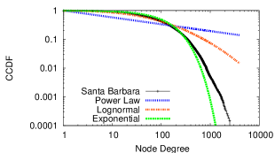
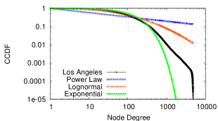
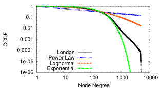
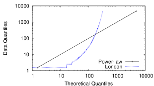
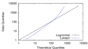
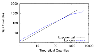
Fitting Models to Real Datasets. We fit each distribution model to our real OSN datasets, using an optimal estimator to derive the best model parameters [11].
For each considered distribution model, we analyze the quality of the fit on our real data through three probability plots: the probability distribution, the complementary cumulative distribution (CCDF), and the “quantile-quantile” plot.
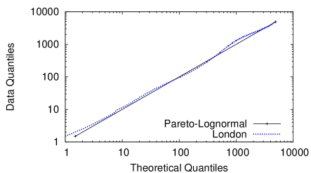
The probability distribution function is an important metric for understanding the portion of nodes that have a certain degree value. For example, the seminal Power-law model predicts that a large number of nodes have a high degree. The CCDF quantifies how often a node’s degree is above a value. It is particularly useful for identifying the general slope of OSN connectivity. Finally, the Quantile-Quantile analysis can graphically compare different distributions, in our case a theoretical model and a real social graph. The plot shows the discrepancy between degree values that correspond to the same quantile in both distributions. The greater the distance from the reference line, the stronger the evidence that the dataset follows a different distribution.
Experimental Results. We perform experiments on our Facebook datasets, the random walk Facebook graph, and the Orkut dataset. Results across all graphs are highly consistent, and we only show 3 graphs for brevity, Santa Barbara Los Angeles and London Facebook networks. These social graphs range in size from K to M nodes.
Figure 2 plots the CCDF of the fitted models on the three datasets. The CCDF presents a detailed view on the tail of these distributions. We see that none of the presented models accurately captures the decay slope shown by the real datasets. Both the Power-law and the Lognormal distributions overestimate the tail. Take London for example (Figure 2). The Power-law model overestimates the highest degree nodes by up to orders of magnitude compared to the real graph. In contrast, the Exponential distribution decays sharply, and significantly underestimates the number of high degree nodes. On the London graph, this error reaches orders of magnitude for nodes with degrees of .
The quantile-quantile plot formally quantifies the distance between the real data and the model. Figure 2 shows that both the Power-law and the Lognormal model underestimate nearly of nodes (i.e. Figure 2, -axis ) and largely overestimate the very high degree nodes. In contrast, the Exponential distribution model exhibits a reasonably good behavior along the lower tail and the body of the distribution compared to the dataset, although a strongly diverging slope is displayed on the high degree nodes.
We do not include plots on the comparison of probability distribution functions because of space constraints. However, they lead to the same conclusion: the high density of nodes with low degree are not well predicted by the Power-law and Lognormal models, and all models fail to accurately predict the number of high degree nodes. Finally, while this section only reports results from graphical assessment of goodness-of-fit, we confirm our observations using statistical error measures later in Section 3.3.
3 Complex distribution models
Our experimental results show that none of the elementary distributions, including the Power-law distribution, provide a satisfactory fit for degree distributions in today’s OSNs. These results, however, do lead to an intuition where low degrees are distributed following a Pareto model while higher degrees can be modeled with an asymptotically faster decaying distribution. We believe a combination of two models will offer a better representation of the complex phenomena observed on the OSNs. Similar approach has been successfully used by other fields, for example, modeling actuarial data in economics [29].
In this section, we test our intuitions by evaluating four distribution models with a Pareto component, each with varying degrees of accuracy and fitting complexity. Ultimately, we confirm via both graphical and statistical analysis that the beginning of these distributions is characterizable as a Pareto and the upper tail decays as a Lognormal, and that the Pareto-Lognormal distribution provides the best combination of accuracy and fitting overhead.
3.1 Pareto with Exponential Cutoff
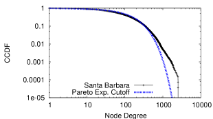
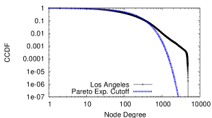
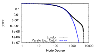
Prior work has proposed modeling human behavior using the Pareto with Exponential cutoff distribution [36], where the beginning of the distribution follows a Pareto and the tail exponentially decays. This formulation is particularly interesting to our study given the decay observed in the tail of our data (see Figure 2). We study this distribution using the derivations from [15].
Fitting to real datasets. Figure 3 shows how well the Pareto with Exponential cutoff distribution fit the Santa Barbara, Los Angeles and London datasets. We plot the CCDF to graphically show how the tail of this distribution decays compared to real datasets. While this model is able to closely fit the low degree nodes of the real data, it fails short in capturing the upper tail by underestimating the density of nodes with high degrees. We conclude that the exponential cutoff is too sharp to properly capture OSN connectivity of central (high-degree) nodes. Intuitively, we are looking for a more gradual decay slope.
3.2 Pareto-Lognormal Distribution
Given the low accuracy in modeling the upper tail of our data with the Pareto with exponential cutoff, we turn our attention to a family of distributions that mixes Pareto with Lognormal distributions. These models, compared to the Pareto with exponential cutoff model, provide a smother decay on the upper tail that provides a better match for our real data. We start with the Double Pareto-Lognormal (DPLN) distribution introduced by Reed in [32]. The DPLN is a complex model with the ability to fuse two Pareto and a Lognormal distribution. It includes four parameters: two Pareto exponents and that identify the slope of the upper and lower tails of the distribution, and and that describe the Lognormal parameters connecting the two Pareto tails. The DPLN also gives rise to two other distributions [32]: the Pareto-Lognormal (PLN) and the Lognormal-Pareto (LNP). Both are expressed by three parameters: Pareto exponent , and Lognormal components and .
Next, we derive the precise formulation of the PLN distribution in terms of the PDF, CDF and the likelihood function. We omit the detailed derivation on DPLN and LNP for brevity. In Section 3.2 and 3.3, we use both graphical and statistical assessments of goodness-of-fit to compare these three distributions.
Pareto-Lognormal PDF and CDF Derivation. The PLN is expressed as the combination of two probability distributions.
We derived the correct formula of this distribution (which is a limit form of the DPLN) using results on the DPLN [32]. The Pareto-Lognormal probability distribution function is:
| (1) |
where characterizes the slope of the lower tail of this distribution which follows a Pareto behavior, and and characterize the body and the upper tail of this distribution, which approximate a Lognormal decline. We also derived the Pareto-Lognormal cumulative distribution function, formalized as follows:
| (2) |
with and . In Section 4, we will analyze the CDF and formally prove that the Pareto component describes the low values of the distribution and the Lognormal one dominates the high values.
Pareto-Lognormal Likelihood Derivation

The likelihood function estimates the parameters of a distribution function in light of the observed data. The likelihood is a function of parameters of the distribution and is defined as follows:
Using the definition of the Pareto Lognormal distribution in Equation 1, the likelihood becomes:
The likelihood is defined as a product, and maximizing a product is usually more difficult than maximizing a sum. Instead, we use a monotonously increasing conversion function to transform the function into a new function , such that and have their maximum values for the same , and values. The monotonous transformation we use is the logarithmic function, which turns the maximization of a product into an easier maximization of a sum. For simplicity, let be , then
| (3) |
We use (3) to estimate the parameters , and in order to fit the Pareto-Lognormal model to our real OSN graphs. We also reverse the sign of (3) such that the likelihood to fit the data is maximized by minimizing .
| Real | Statistical | Distribution Models | ||||||
| Graph | Methods | Power-law | Lognormal | Exponential | Pareto-Exp. | LNP | PLN | DPLN |
| Monterey | Log L. | 8.75338e+04 | 7.83008e+04 | 7.78214e+04 | 7.76411e+04 | 7.76411e+04 | 7.74057e+04 | 7.74089e+04 |
| nodes | AIC | 1.75069e+05 | 1.56605e+05 | 1.55644e+05 | 1.55188e+05 | 1.55288e+05 | 1.54817e+05 | 1.54825e+05 |
| edges K | RSS | 3.05267e+02 | 2.07443e+00 | 4.86935e-01 | 3.43766e-01 | 2.59320e-01 | 2.26463e-02 | 2.32905e-02 |
| Santa Barbara | Log L. | 1.80247e+05 | 1.63328e+05 | 1.61209e+05 | 1.60516e+05 | 1.61152e+05 | 1.60448e+05 | 1.60455e+05 |
| nodes | AIC | 3.60497e+05 | 3.26660e+05 | 3.22421e+05 | 3.21036e+05 | 3.22311e+05 | 3.20902e+05 | 3.20919e+05 |
| edges M | RSS | 4.38954e+02 | 5.81415e+00 | 7.31640e-01 | 3.37774e-01 | 6.10471e-01 | 7.44256e-02 | 7.74719e-02 |
| Egypt | Log L. | 1.62073e+06 | 1.53376e+06 | 1.53832e+06 | 1.50289e+06 | 1.49892e+06 | 1.49855e+06 | 1.49830e+06 |
| nodes K | AIC | 3.24148e+06 | 3.06754e+06 | 3.07664e+06 | 3.00579e+06 | 2.99785e+06 | 2.99710e+06 | 2.99661e+06 |
| edges M | RSS | 1.17928e+03 | 7.68335e+00 | 1.69934e+00 | 3.43834e-01 | 2.13671e-01 | 1.58090e-01 | 2.03417e-01 |
| Los Angeles | Log L. | 3.81640e+06 | 3.45975e+06 | 3.44290e+06 | 3.42677e+06 | 3.41280e+06 | 3.40372e+06 | 3.40379e+06 |
| nodes K | AIC | 7.63281e+06 | 6.91950e+06 | 6.88581e+06 | 6.85354e+06 | 6.82561e+06 | 6.80745e+06 | 6.80759e+06 |
| edges M | RSS | 1.74060e+03 | 8.60777e+00 | 1.50800e+00 | 8.55362e-01 | 5.02215e-01 | 4.82168e-02 | 4.75582e-02 |
| New York | Log L. | 5.66194e+06 | 5.23512e+06 | 5.17802e+06 | 5.12808e+06 | 5.13177e+06 | 5.11728e+06 | 5.11753e+06 |
| nodes K | AIC | 1.13239e+07 | 1.04702e+07 | 1.03560e+07 | 1.02561e+07 | 1.02635e+07 | 1.02345e+07 | 1.02350e+07 |
| edges M | RSS | 1.81230e+03 | 1.65956e+01 | 1.87038e+00 | 5.88628e-01 | 7.90849e-01 | 1.70891e-01 | 1.65433e-01 |
| Manhattan R.W. | Log L. | 6.76810e+06 | 5.92193e+06 | 5.86365e+06 | 6.02838e+06 | 5.89459e+06 | 5.85632e+06 | 5.85679e+06 |
| nodes K | AIC | 1.35362e+07 | 1.18438e+07 | 1.17273e+07 | 1.20567e+07 | 1.92208e+07 | 1.17126e+07 | 1.17135e+07 |
| edges M | RSS | 1.31910e+03 | 4.01862e+00 | 9.62000e-02 | 8.07448e+00 | 6.29269e-01 | 2.44948e-02 | 2.34597e-02 |
| London | Log L. | 1.07131e+07 | 9.75799e+06 | 9.60413e+06 | 9.65522e+06 | 9.61043e+06 | 9.56562e+06 | 9.56626e+06 |
| nodes M | AIC | 2.14262e+07 | 1.95159e+07 | 1.92082e+07 | 1.92104e+07 | 1.17892e+07 | 1.91312e+07 | 1.91325e+07 |
| edges M | RSS | 1.79927e+03 | 1.24657e+01 | 7.33091e-01 | 2.30840e-01 | 1.26502e+00 | 1.99847e-01 | 2.12646e-01 |
| Orkut | Log L. | 1.81346e+07 | 1.63179e+07 | 1.62442e+07 | 1.61573e+07 | 1.61822e+07 | 1.60868e+07 | 1.60829e+07 |
| nodes M | AIC | 3.62692e+07 | 3.26358e+07 | 3.24885e+07 | 3.23147e+07 | 3.23645e+07 | 3.21738e+07 | 3.21659e+07 |
| edges M | RSS | 1.94280e+03 | 2.41064e+00 | 3.75274e-01 | 2.95699e-01 | 4.16978e-01 | 1.60096e-02 | 1.01767e-02 |
Parameter estimation. The Pareto-Lognormal distribution has three parameters (i.e. , and ) to estimate in order to fit real data. We perform a grid search, i.e. a multi-dimensional numerical search over the parameters space, to identify the best triplet of values to fit a particular dataset, as in [35].
We bound the search of the parameters and using the Moment Method Estimation to determine the initial values, and then refine the search around those values to identify the best ones. While this methodology could lead to suboptimal results that lower the performance of our models when compared to those using optimal parameter configurations, we choose it because of its computational efficiency.
We use the likelihood metric as the objective function in our parameter search [6], i.e. our goal is to minimize the reverse log likelihood “” when searching for the optimal (, , ) [6]. To show that there is a clear concave trend around the minima, we plot in Figure 4 the values of for the London dataset as a function of . We have identified similar trends in all our datasets.
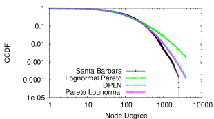
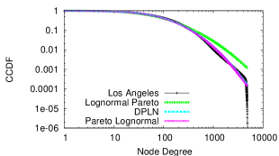
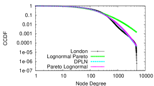
Fitting to real datasets. Figure 5 examines the results of fitting the PLN, DPLN and LNP distributions to our graphs as CCDF plots. Among these three models, LNP overestimates the data on the upper tail, which suggests that the decay of the right tail follows more of a Lognormal model than a Pareto one. The flexibility of the DLPN model, with its four parameters, allows for a very good fit. However, it comes at the cost of a higher fitting complexity which grows exponentially in the number of parameters. On the other hand, the PLN distribution achieves the accuracy of the DPLN, and also has the reduced fitting complexity of LNP (i.e. 3 parameters instead of 4). Figure 5 clearly shows that on all three datasets (i.e. Santa Barbara, Los Angeles and London), PLN and DPLN overlap along the entire distribution. In addition, we use the Quantile-Quantile plot to evaluate the fitting accuracy of PLN, and show the results for London in Figure 6. This plot is representative and others are omitted for brevity. It shows a near perfect fitting from the Pareto-Lognormal to the real London graph.
3.3 Statistical Analysis
The graphical assessments in Section 2 (i.e. the PDF, CCDF and the Quantile-Quantile plot) are the first step towards a complete characterization of these distributions. We now look at statistical measures to quantify how well each model fits real social graphs [10].
Goodness-of-Fit Analysis. We consider three measures to evaluate the goodness of the proposed statistical models, including the likelihood function, the Akaike’s Information Criterion and the Residual Sum of Squares.
The likelihood function is used to quantify the likelihood that a particular model fits a given dataset. Section 3.2 explained how to estimate this function for PLN by computing the minimum of the reverse log likelihood. We compute the minimum of the reverse of the log likelihood function for each model such that the best fit models generate the lowest values. This matches the two other measures, where the best models also generate the smallest fitting errors.
Akaike’s Information Criterion (AIC) [3] is a measure of the quality of the fit that is capable of capturing the tradeoff between accuracy and fitting costs. The AIC value is computed as: where is the number of parameters in the statistical model, and is the maximized value of the likelihood function for the estimated model. The value in the AIC test is used to tradeoff the accuracy of a model with its complexity. The model that shows the lowest AIC is considered the one that best fits the data.
Residual Sum of Squares(RSS) [35] is a statistical method that computes the sum of squares of residuals between the empirical distribution and the data sample. It measures the discrepancy as euclidean distance between the data and the estimation model. A small RSS indicates a tight fit of the model to the data, and it can be formally expressed as: , where is the empirical evaluation and is the estimate value of the statistical model.
Error Measures on Real Traces. We now compare models based on the numerical values of these three statistical methods computed on our OSN datasets. We explore sample size variation to prove that the datasets manifest the same trend across different sample sizes.
In Table 1 we report a set of statistical values to quantify the goodness-of-the-fit for each of the seven analyzed models. We highlight in bold the smallest values (i.e. those that identify the best model) for each metric.
Across all datasets, the Power-law model consistently performs the worst. Its values of Log Likelihood and AIC test are the highest and the RSS values are up to orders of magnitude higher than the best model. The second worst model on our measured datasets is the Lognormal. Its RSS values are up to order of magnitude larger than the best model, due to the high imprecision in estimating the high degree nodes. Exponential, Pareto with Exponential cutoff and LNP provide reasonable accuracy in the sense their values are with order of magnitude from the best.
The two best models are DPLN and PLN. The RSSs for some datasets identify DPLN as the best model, with a very small difference separating it from PLN (on the second or third decimal point). On the other side, the AIC test slightly penalizes the model with more parameters, such as DPLN. Based on the results of both the likelihood and the AIC, we see that PLN does consistently well on all our Facebook datasets. Finally, analysis of the Orkut graph produces results consistent to our Facebook graphs.
Overall we see a consistent trend: Power-law does not produce accurate results, and the best models are PLN and DPLN. Only in a small number of cases, DPLN is slightly more accurate than PLN, but differences are exceptionally small compared to other models. Given the significant increase in fitting complexity for DPLN (i.e. deriving 4 rather than 3 parameters), the PLN model clearly produces the best combination of fitting accuracy and complexity.
4 Implications of the PLN model
We have shown that the PLN model provides a much more accurate fit to today’s OSN graphs. But are these differences large enough to really matter? In this section, we answer this question by quantifying the magnitude of error introduced by the Power-law model, and in the process, show that social algorithms and protocols based on the Power-law assumption must be re-evaluated (and some re-designed) using the PLN model.
The remainder of this section includes three parts. First, we analyze PLN using its CDF to characterize the asymptotical slope of its tail, which we use later to derive more complete bounds, in order to better understand the high degree nodes of these networks. Second, for both PLN and Power-law model, we analytically determine a close form to bound the lowest degree of high degree nodes. By comparing these bounds, we formally quantify the divergence of Power-law from PLN. We also validate our analytical results from empirical analysis on our Facebook and Orkut graphs. Finally, for both models, we approximate the cardinality of high degree nodes (those with degrees in the top 10% of the network), and evaluate the discrepancy between the two. Again, we validate our analytical results using our real datasets to understand the actual prediction errors from both models.
4.1 Modeling High Degree Nodes with PLN
The cardinality of high degree nodes is a key factor in designing social applications and protocols. To characterize this distribution in the PLN model, it is necessary to understand the limit behavior on its CDF (or ), defined by (2). We aim to bound the limit behavior so that we can directly derive the expected number of high degree nodes and their connectivity. Let , , we have
| (4) |
Leveraging the erf function (i.e. the Gauss error function, which is a special function of sigmoid shape), we can express the standard normal cumulative distribution and its complementary form respectively as follows:
| (5) |
| (6) |
with . Note that by definition, and . We can now reformulate (4) through the use of Gauss error functions as:
| (7) |
Next we use the asymptotical expansion of the Gauss error function to further expand . For large , the function can be approximated with the following series:
| (8) |
Without loss of generality, in the remainder of this analysis, we will only use the first term of the series in (8). This is because it achieves enough accuracy to accomplish the goals of this investigation. While we omit a formal error analysis of the loss in the approximation, we will show via experimental analysis that the loss is negligible, and the results are sufficiently accurate. Thus the function is approximated as follows:
| (9) |
Lemma 1
[32] For a sufficiently large , goes to .
The claim states that for large the PLN distribution has a Lognormal form with the parameters of the PLN model. We will use this Lemma extensively in the following discussions.
4.2 Quantile Analysis: a Degree Threshold
Next, we quantify how well the PLN and the Power-law models predict the degree threshold that defines the top subset of the highest degree nodes in the network. In other words, we wish to predict the minimum degree , such that nodes with degree are in the top portion of all nodes sorted by degree. Formally, is the -th quantile of the complementary cumulative distribution. As a concrete example, we will use , i.e. top 10%.
We compute for both models. For the Power-law model, the degree can be expressed as: . To quantify the same quantile for the PLN distribution, we again leverage its limit behavior. We then use the asymptotic expansion of the complementary Gauss error function to obtain a tight upper bound in Lemma 2.
Lemma 2
A tight upper bound of the -th quantile of the PLN distribution is .
Proof 4.1.
Given the result in Lemma 1, we consider for large values of . Since we are
using the Pareto-Lognormal parameters, we can reformulate the
complementary cumulative distribution function for large
values as:
.
In order to derive the minimum degree , which characterizes
the high degree nodes, we first quantify the % of high degree
nodes in the network, and then derive the required degree value. We
leverage the tail of the complementary cumulative distribution from
Lemma 1, and thus, the following holds:
| (10) |
Let , then (10) becomes . Applying the logarithmic function and approximation with the quadratic term, it reduces to . By substituting , we have or which is the minimum degree of the high degree nodes in the -th quantile.
Next, we approximate the differences among the quantiles between the PLN and the Power-law distributions. Note that we are not approximating through a limit formulation but we are estimating the difference of the two, i.e. PLN and Power-law, analytical quantile values when . In order to compute the difference of the estimated by the Power-law and the PLN, we approximate the PLN’s as , since is negligible compared to when is around its typical value .
The Power-law overestimation can be computed as the ratio of the quantiles of the Power-law and the PLN. Since and are approximated by the mean value, , of the sample logarithms, the following theorem applies:
Theorem 4.2.
For , the ratio of the quantiles of the Power-law and PLN is .
Both the PLN and Power-law estimates will express the degree as an exponential function, but they have different bases. For the Power-law, the base of the exponent is ; for PLN it is . This discrepancy accounts for the large difference in the predictions made by the two models. As we will show using experimental validation on real datasets, this difference can be as large as two order of magnitude.
| Real | (see Lemma ) | ||
|---|---|---|---|
| Graphs | Power-law | PLN | Real Data |
| Monterey | 8906 | 582 | 246 |
| Santa Barbara | 160362 | 845 | 345 |
| Egypt | 29987 | 775 | 206 |
| Los Angeles | 170457 | 1101 | 363 |
| New York | 152937 | 1099 | 395 |
| Manhattan R.W. | 357804 | 797 | 583 |
| London | 176742 | 939 | 364 |
| Orkut | 41377 | 369 | 155 |
Experimental Validation on Real Data. Now we aim to validate the theoretical result shown in the previous section using experimental analysis on our datasets. For each dataset presented in Table 1, we compute its value (i.e. the estimated minimum node degree within the % of the highest degree nodes), and compare them against their analytical bounds from the PLN (see Lemma 2) and Power-law models.
We list the results in Table 2. Clearly, our theoretical approximation of values using PLN are consistently more accurate than those from the Power-law model, which over-estimates the real data up to orders of magnitude. For instance, on the New York graph, the value from the real sample is ; our theoretical approximation from PLN is ; but the Power-law predicts .
4.3 Cardinality of High-degree Nodes
We next use the distribution models to predict the cardinality of high-degree nodes in OSN graphs. The cardinality of high-degree nodes is commonly used to design social algorithms and protocols, and to evaluate their performance and complexity. In the following, we first analytically quantify this metric using both the Power-law and PLN models, and then empirically validate our predictions using real datasets.
Power-law model. Using the Power-law density function, we can derive the number of high degree nodes by computing the integral of the upper tail of the distribution. Let be the minimum node degree among the high degree nodes, then the number of high degree nodes is approximated as:
| (11) |
where is the normalization constant, approximated by , and is the minimum node degree in the network.
PLN model. As mentioned before, a high degree node has a degree at least , where can be computed as in Section 4.2. Thus, the next lemma follows:
Lemma 4.3.
Let be the minimum degree for a high degree node, then the number of high degree nodes .
Using Lemma 1, the number of high degree nodes described by the PLN distribution can be studied from the component of the CCDF of the PLN, where is . Thus this number becomes: . Using the approximation in (8), we approximate the number of nodes in the network with degree no less than by
| Real | # of nodes with degree | ||
|---|---|---|---|
| Graphs | Power-law | PLN | Real Data |
| Monterey | 1843 | 1387 | 1385 |
| Santa Barbara | 6763 | 2442 | 2724 |
| Egypt | 61170 | 30387 | 28319 |
| Los Angeles | 141980 | 54894 | 57182 |
| New York | 204540 | 77879 | 85581 |
| Manhattan R.W. | 76133 | 76133 | 72854 |
| London | 398529 | 156850 | 160050 |
| Orkut | 761970 | 334900 | 307240 |
Comparing High-degree Node Cardinality and Connectivity.
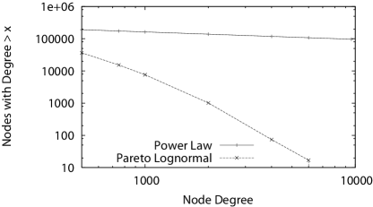
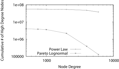
We use two experiments to validate the quality of predictions on high-degree nodes from PLN and Power-law. First, we study the number of high-degree nodes in the measured network datasets, and compare this number with that estimated from the fitted models in Table 3. Specifically, we study the total number of high-degree nodes, defined as the nodes with degree higher than generated from the top of the network as proven in Section 4.2.
Table 3 shows the cardinality of high-degree nodes in the measured networks, as well as those predicted by the PLN and Power-law models. Clearly, the PLN model provides a tight approximation of the real dataset values, while predictions made by the Power-law model generally lead to more than % estimation error.
Empirical results like these can sometimes be biased because of specific distributions in the real data. To eliminate any possible bias, we generate pure sample networks from the Pareto-Lognormal and the Power-law models, then compute and compare each model’s predicted number of high degree nodes and their connectivity.
The pure sample networks are generated as follows. For the Power-law, we take the parameters of a fitted model on a particular real sample, and generate a pure sample by uniformly extracting numbers between and . Then for each extraction , a node with the following degree is generated: , where has the value of the Power-law exponent fitted on a real dataset. For the Pareto-Lognormal, we generate a pure sample as follows: let be a random number uniformly extracted between and , and let be a random number from the exponential distribution with mean parameter . Then , where , and are the parameters of the Pareto-Lognormal fitted on the real dataset. In Figures 7 and 8, we compare the number of high degree nodes and the sum of all node degrees respectively. We do this for , and use the average of the fitted model values as the parameters of the Power-law and the Pareto Lognormal. Figure 7 shows the divergence of these two models in estimating the high degree nodes. In particular for nodes with degree , Power-law generates orders of magnitude more nodes than PLN.
5 Impact on Social Applications
In the last section, we argued using both analytical predictions and empirical data that the Pareto-Lognormal model provides a much more accurate representation of node degree distributions in OSNs. In this section, we seek to better understand how the choice of degree distribution model impacts the performance of applications on social graphs. More precisely, for applications that run on social graphs, we wish to quantify just how much the choice of a degree distribution model alters their experimental results.
When actual measured social graphs are not available, social applications generally use synthetic graphs generated using statistics extracted from real graphs [9]. To highlight the differences when applications use either the Pareto Lognormal or the Power-law degree model, we take each of our real Facebook social graphs, and generate two synthetic versions of them: one assuming a PLN model for degree distribution, and one assuming Power-law. We generate these synthetic graphs using prior works from [26, 7], which can generate a synthetic graph with no self loops, given a specified degree distribution and a given network size.


We present results from implementations of three important applications on social graphs. They include: a) a graph partition approach that replicates high degree nodes across partitions (introduced in Section 1), b) influence maximization on social graphs using three different information spread models [9], and c) a link-privacy attack on anonymized social graphs [17].
All results are computed on a local cluster of Dell Xeon servers with 24–32GBs of main memory. Memory constraints limited the size of graphs we used in our results. Using Amazon EC2 large memory machines, we verified that our observed trends hold for larger graphs such as the Orkut graph, but such computations were too slow and costly in resources for us to generate comprehensive graphs.
5.1 Partitioning via Supernode Replication
Efficiently answering queries on large graphs is a difficult challenge faced by companies dealing with large network datasets, e.g. Facebook, Zynga. Scalable solutions require splitting the graph data across machines in computing clusters. While some systems [30, 12] distribute nodes randomly across a cluster, an ideal solution would find a way to distribute the graph across the cluster as subgraphs with minimal edges between them. The best solutions would minimize edges between partitions, which minimizes data dependencies between machines and maximizes parallel query processing.
Unfortunately, graph partition is known to be NP-Complete [5], and social graphs are known to be very dense graphs that do not partition well. Fortunately, Power-law networks are known to be vulnerable to “targeted attacks,” i.e. they quickly fragment into disconnected subgraphs when nodes with the highest degree are removed [4]. Since social graphs are widely accepted as Power-law graphs, we hypothesize we can easily partition a social graph by first fragmenting it into subgraphs, through the removal of a small number of supernodes. These supernodes (and their edges) can be replicated to every node in a cluster. In addition to potentially partitioning highly connected graphs, this approach is attractive because it does not require the entire graph to be in memory, and can thus efficiently run on extremely large social graphs.
We now look at the impact of running this partition scheme both on real social graphs, and on synthetic graphs generated using the Power-law and PLN synthetic models. We take three of our social graphs, the Facebook regional graphs from Santa Barbara, CA, USA and London, UK [39], and the Orkut social graph [23], and create synthetic graphs that match each of them in size and node degrees, based on either the Power-law or the PLN model for degree distributions. We generate synthetic graphs from degree distributions using Newman’s approach [26].
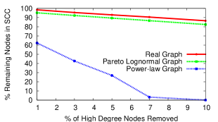
For each of these graphs, we test the effectiveness of our graph partitioning strategy, by incrementally removing nodes from the graph, starting with those nodes with the highest degree. After these super nodes are removed, we examine the remaining graph, and measure the size of the largest connected component as a function of the original full graph.
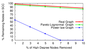
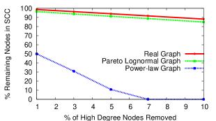
We plot the results in Figure 9 for each of the original graphs. The results are strongly consistent among our datasets. Regardless of the original graph in question, synthetic graphs produced using a Power-law distribution are quickly fragmented. Removing just the top 3% of the highest degree nodes reduces the largest connected component to only of the original graph. In contrast, the real social graphs and synthetic graphs from the Pareto-Lognormal distribution are highly resistant to the fragmentation. Even after removing of the highest degree nodes, the graph remains largely connected, and the biggest connected component still contains of all nodes. In this case, relying on an inaccurate degree distribution model produces results fundamentally different from the original graph.
5.2 Influence Maximization
Social networks have proven to be exceptionally useful tools for information dissemination and marketing, and are used by companies and individuals to promote their ideas, opinions and products. One critical problem of interest is that of influence maximization, or how to identify an initial set of users who can influence the most number of users. This is known as the influence maximization problem.
We examine the impact of degree distribution models on the influence maximization problem. Prior works have provided algorithms that use statistical methods to model information dissemination over social links [9, 16]. We consider three different models to spread information: independent cascade model, weighted cascade model and linear threshold. These models differ in how they compute the probability of influencing a node in the graph. For example, independent cascade assumes a node is influenced independently from nearby nodes, while the probability of a node in weighted cascade being influenced is a function of its degree. In each case, heuristics provided by [9] allow us to compute the number of users influenced by an initial set of “seed” users. We seek to understand how the spread of influence in these models is impacted by the structure of the network. We take the Santa Barbara Facebook graph, its two synthetic variants based on Power-law and PLN, and compute how many users are influenced as the number of seed nodes increases for each of the three influence models mentioned above. We focus on results from the Santa Barbara network, since it is the largest graph we can execute given the significant memory footprint of code from [9]. Prior work has shown this graph to be a representative social graph in all graph metrics [33].
Figure 10 shows the spread of information for each of the three different models on the Santa Barbara network. For each model, we compare the results on Santa Barbara with results on its Power-law and PLN synthetic graphs. Our results are consistent across all three influential models. While the exact result differs for each particular influential model, results from the PLN graph results always closely follow results from the real graph. In contrast, results on the Power-law graphs always overestimate the number of influenced users on the real graph, sometimes overestimating by an order of magnitude. These results are further confirmation that using an inaccurate degree distribution model can introduce dramatic errors in application-level experimental results.

5.3 Attacks on Link Privacy
For our third application study, we focus on the problem of link privacy in social graphs. Prior studies such as [17] used experiments to quantify the impact of attacks to disclose the presence of connections between social network users. This example differs from our other application studies in that the application results are simulated based on analytical derivations that integrate a degree distribution model.
[17] presents different approaches to disclosure network information by attacking particular nodes in the network. The most effective attack strategy is “Highest,” which tries to compromise nodes by spreading the attack from high degree nodes. Intuitively, because high degree nodes have many incident edges, they are more likely to successfully spread the attack across other nodes. The authors provide a mathematical form to quantify the effect of this attack by using a probabilistic approach that leverages the probability distribution function of the network111 This use of network topology models is also commonly used in problems involving information propagation or dissemination in social networks.. This leads to a simple question: how much does the effectiveness of this attack depend on the choice of network topology model?
Quantifying the strength of this attack relies a notion of node coverage. A node is covered if and only if its -hop neighbors are unequivocally known. This definition allows [17] to present results where the strength of this attack is quantified as the fraction of nodes whose entire immediate neighborhood is known.
Let us begin by introducing the required variables to repeat the experiment: , and are respectively the total number of nodes in the networks, the sum of the node degrees and the minimum degree. The variable identifies the sum of the degree of the nodes from where the attack originates. Theorem in [17] states that if , then the disclosed nodes after the attack are: . is a variable that we can compute as follows: let , which is needed to estimate the fraction of covered nodes. We can derive as:
where is the maximum node degree, is the degree of and is the density function of the degree distribution. If we assume a Power-law degree distribution, we substitute with and in the case of the Pareto-Lognormal we use as defined in (1).
Figure 11 shows that results on a Power-law network significantly overpredicts the impact of attacks using the “Highest” strategy. In contrast, results on the real social graph closely match those from a synthetic graph following the Pareto-Lognormal degree model. Clearly, applications that use the Power-law model in their analytic derivations and simulations are also significantly affected by their choice of node degree distribution models.
6 Towards a Generative Model
In this section, we present preliminary results towards a generative model able to reproduce a Pareto Lognormal graph. We also show using evidence in our datasets that the formation of these graphs diverges from the hypothesized preferential attachment-based scheme presented in prior studies [37, 21].
Our goal is to provide an intuition of an algorithm that captures a lognormal multiplicative process, and accurately models the temporal evolution of online social networks. Unlike generative models that focus on reproducing a single snapshot of a network [21], we focus on modeling the evolutionary process that captures the network growth. While the Power-law curve is generated by an iterative process following the preferential attachment rule, our PLN model may be explained by the following process: “A node joins the network through an introduction node, and builds connections within the local community; then it completes its growth by joining and growing in multiple other communities.” To realize a generative model based on this intuition, we need a stochastic process derived from the PLN distribution that balances the Pareto and the Lognormal process to drive the growth rate of each node.
Dynamic Graph Snapshots. To understand the growth of social networks, we perform daily crawls of the San Francisco Facebook network during the month of November . We use the same crawling strategy used to capture other Facebook datasets [39]. We use these daily snapshot graphs to help us understand the rate of network growth and how new edges form.
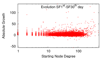
Network Generative Models. Since our PLN model is itself a combination of a Pareto distribution and a Log-normal distribution, our search for an iterative process should naturally integrate two theories. Starting with “Preferential Attachment” [37], which produces a Power-law distribution, we add the “Law of Proportional Effects” [13], where the growth of the degree of a node, at discrete time , is multiplicative and independent from its actual size . This contributes to a Lognormal distribution. We study the correlation of growth and current degree using our 30 snapshot graphs of the San Francisco network. The results in Figure 12 confirm that the degree growth of different nodes is not influenced by their starting degree, meaning that the growth is a constant independent of node degrees.
A Two-Phase Iterative Algorithm. We envision a two-phase iterative algorithm that integrates fundamental properties from the “Law of Proportional Effects” [13] and “Preferential Attachment” [37]. The bimodal connotation is meant to highlight the ability of our algorithm to integrate the Power-law and Lognormal probability models.
Our two-phase algorithm alternates between adding new nodes to the network using a preferential attachment model, and growing the connectivity among nodes using the law of proportionate effects. Its two phases are driven by a probability parameter . We do not claim to provide a formal derivation of the algorithm or its proof of correctness. Both are beyond the scope of this paper. Here we limit ourselves to preliminary results to validate our underlying intuition.
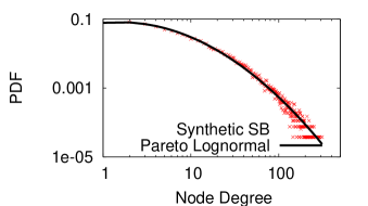
Initial Validation. To evaluate our intuition about the generative method, we implement a simple instance of a “Two-Phased Iterative Algorithm” summarized above, and run a structural comparison between the generated graphs and the real social network graphs. We fit the parameters of this algorithm by following the approach presented in [33].
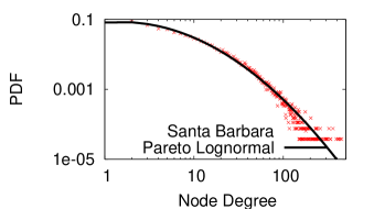
Our goal is to show that our intuitive algorithm for generating PLN distributions can generate synthetic graphs that accurately reproduce the degree distribution of our real data. In Figure 13, we show the similarity between the pdf of node degrees from the real data, versus those from the synthetic graph produced by our algorithm. The results are consistent across all seven of our datasets, and we only show results only on Santa Barbara Network for brevity222These synthetic graphs also show similar structural characteristics to the original graphs, including clustering coefficient, Knn, separation metrics, and betweenness centrality.. Given these initial results, we are continuing to work on formalizing the mathematical formulation of our generative model and a more thorough analysis via larger, more complete synthetic datasets.
7 Related Work
Social Networks. Historically, both online and offline social networks have been explained through the seminal Power-law model. Power-law is often described with the “rich gets richer” paradigm which has been proven to hold in real datasets across multiple disciplines, including Internet router topology graphs, biological graphs [11, 31], human mobility traces [8], etc.
One of the first OSN study was conducted on Club Nexus website [1]. Later analytical studies attracted attention for their large scale, including CyWorld, MySpace and Orkut [2], YouTube, Flickr, LiveJournal in [23], and the most recent studies of Facebook [39] and Twitter[19]. More recently, researchers have begun to investigate the temporal properties of OSNs [18, 24, 22].
Preliminary analysis of OSN structures in these and other studies has shown that the degree distribution does not follow a pure Power Law distribution. As a result, followup work proposed to segment these distributions and fit the segmented pieces with distinct Power-law settings [14, 2].
Social Applications and Systems. We have shown that our proposed PLN is statistically more accurate in describing OSNs than the seminal Power-law model. We believe that many social applications and protocols designed based on the Power-law assumption need to be re-evaluated, especially algorithms and protocols that rely on the population of high degree nodes or their connectivity. Examples include distributed resource replication strategies to minimize routing delay and social search, epidemics dissemination strategies to maximize information spread [9], landmark selection strategies to accurately predicts shortest paths in graphs [28], community detection to improve social recommendation systems, and social attack strategies [17].
8 Conclusion
Degree distributions are incredibly important tools for studying and understanding the structure and formation of social networks. They give us insight into network structure, and are the foundations of generative models that model growth and network dynamics [36, 20, 21]. Finally, they are key tools in the design and analysis of efficient algorithms for a number of challenging graph problems.
Our work sheds light on an existing discrepancy between the commonly used Power-law model and real measurement data from today’s online social networks. While most prior studies have ignored this error, we show that it is consistent across different communities and propose the Pareto-Lognormal distribution (PLN) as a more accurate alternative. Our analysis shows that PLN significantly outperforms existing elementary models, and is the most accurate and efficient of all complex distribution models we studied. Finally, we analytically quantify the magnitude of error reduction achieved by moving from the Power-law to the PLN model, and confirm our analysis with empirical data.
References
- [1] Adamic, L. A., Buyukkokten, O., and Adar, E. A social network caught in the web. First Monday 8, 6 (2003).
- [2] Ahn, Y.-Y., et al. Analysis of topological characteristics of huge online social networking services. In Proc. of WWW (2007).
- [3] Akaike, H. A new look at the statistical model identification. IEEE Transactions on Automatic Control 19, 6 (1974), 716 – 723.
- [4] Albert, R., Jeong, H., and Barabasi, A.-L. Error and attack tolerance of complex networks. Nature 406 (July 2000).
- [5] Andreev, K., and Räcke, H. Balanced graph partitioning. In Proc. of SPAA (2004).
- [6] Arnold, B. C. Pareto distribution. Encyclopedia of Statistical Sciences. John Wiley & Sons, Inc. (2004).
- [7] Britton, T., Deijfen, M., and Martin-Lf, A. Generating simple random graphs with prescribed degree distribution. Journal of Statistical Physics 124, 1377–1397.
- [8] Chaintreau, A., et al. Impact of human mobility on opportunistic forwarding algorithms. IEEE Transactions on Mobile Computing 6, 6 (2007), 606–620.
- [9] Chen, W., Wang, Y., and Yang, S. Efficient influence maximization in social networks. In Proc. of KDD (2009).
- [10] Claeskens, G., and Hjort, N. L. Model selection and model averaging. Cambridge University Press (October 2008).
- [11] Clauset, A., et al. Power-law distributions in empirical data. SIAM Review 51, (4) (2009), 661–703.
- [12] Dean, J., and Ghemawat, S. Mapreduce: Simplified data processing on large clusters. In Proc. of OSDI (December 2004).
- [13] Gibrat, R. La loi de l’effet proportionnel. Compte-Rendus de l’Acadamie des Sciences (1932), 843–845.
- [14] Gjoka, M., Kurant, M., Butts, C. T., and Markopoulou, A. Walking in Facebook: A case study of unbiased sampling of OSNs. In Proc. of INFOCOM (2010).
- [15] Kagan, Y. Y., and Schoenberg, F. Estimation of the upper cutoff parameter for the tapered pareto distribution. Journal of Applied Probability, Vol. 38 (2001), 158–175.
- [16] Kempe, D., Kleinberg, J. M., and Tardos, E. Maximizing the spread of influence through a social network. In Proc. of KDD (2003).
- [17] Korolova, A., et al. Link privacy in social networks. In Proc. of CIKM (2008).
- [18] Kumar, R., et al. Structure and evolution of online social networks. In Proc. of KDD (2006).
- [19] Kwak, H., Lee, C., Park, H., and Moon, S. What is twitter, a social network or a news media? In Proc. of WWW (2010).
- [20] Leskovec, J., et al. Microscopic evolution of social networks. In Proc. of KDD (2008).
- [21] Leskovec, J., and Faloutsos, C. Scalable modeling of real graphs using kronecker multiplication. In Proc. of ICML (2007).
- [22] Leskovec, J., Kleinberg, J., and Faloutsos, C. Graphs over time: Densification laws, shrinking diameters and possible explanations. In Proc. of KDD (2005).
- [23] Mislove, A., et al. Measurement and analysis of online social networks. In Proc. of IMC (Oct 2007).
- [24] Mislove, A., et al. Growth of the flickr social network. In Proc. of WOSN (Seattle, WA, August 2008).
- [25] Mitzenmacher, M. A brief history of generative models for power law and lognormal distributions. Internet Mathematics 1, 2 (2003).
- [26] Newman, M. E. J., Strogatz, S. H., and Watts, D. J. Random graphs with arbitrary degree distributions and their applications. Phys. Rev. E 64, 2 (2001), 026118.
- [27] Pennock, D. M., Flake, G. W., Lawrence, S., Glover, E. J., and Giles, C. L. Winners don’t take all: Characterizing the competition for links on the web. In PNAS (2002), pp. 5207–5211.
- [28] Potamias, M., et al. Fast shortest path distance estimation in large networks. In Proc. of CIKM (2009).
- [29] Preda, V., and Ciumara, R. On composite models: Weibull-pareto and lognormal-pareto. - a comparative study -. Journal for Economic Forecasting 3, 2 (2006), 32–46.
- [30] Pujol, J. M., et al. The little engine(s) that could: scaling online social networks. In Proc. of SIGCOMM (2010).
- [31] Qian, J., N, M. L., and Gerstein, M. Protein family and fold occurrence in genomes: power-law behavior and evolutionary model. Journal of Molecular Biology 313, 4 (2001), 673 – 681.
- [32] Reed, W. J., and Jorgensen, M. The double pareto-lognormal distribution - a new parametric model for size distribution. Com. Stats – Theory & Methods 33, 8 (2004), 1733–1753.
- [33] Sala, A., Cao, L., Wilson, C., Zheng, H., and Zhao, B. Y. Measurement-calibrated graph models for social network experiments. In Proc. of WWW (Raleigh, NC, April 2010).
- [34] Saroiu, S., Gummadi, K., and Gribble, S. D. A measurement study of peer-to-peer file sharing systems. In Proc. of MMCN (2002).
- [35] Seshadri, M., Machiraju, S., Sridharan, A., Bolot, J., Faloutsos, C., and Leskovec, J. Mobile call graphs: beyond power-law and lognormal distributions. In Proc. of KDD (2008).
- [36] Trevor, F., Mark, L., and George, L. A stochastic evolutionary model exhibiting power-law behaviour with an exponential cutoff. Physica A Statistical Mechanics and its Applications (2005), 641–656.
- [37] Vazquez, A. Growing network with local rules: Preferential attachment, clustering hierarchy, and degree correlations. Physical Review E 67-056104 (2003).
- [38] Viswanath, B., Mislove, A., Cha, M., and Gummadi, K. P. On the evolution of user interaction in Facebook. In Proc. of WOSN (2009).
- [39] Wilson, C., Boe, B., Sala, A., Puttaswamy, K. P. N., and Zhao, B. Y. User interactions in social networks and their implications. In Proc. of EuroSys (April 2009).