Bayesian Methods for Analysis and Adaptive Scheduling of Exoplanet Observations

Abstract

We describe work in progress by a collaboration of astronomers and statisticians developing a suite of Bayesian data analysis tools for extrasolar planet (exoplanet) detection, planetary orbit estimation, and adaptive scheduling of observations. Our work addresses analysis of stellar reflex motion data, where a planet is detected by observing the “wobble” of its host star as it responds to the gravitational tug of the orbiting planet. Newtonian mechanics specifies an analytical model for the resulting time series, but it is strongly nonlinear, yielding complex, multimodal likelihood functions; it is even more complex when multiple planets are present. The parameter spaces range in size from few-dimensional to dozens of dimensions, depending on the number of planets in the system, and the type of motion measured (line-of-sight velocity, or position on the sky). Since orbits are periodic, Bayesian generalizations of periodogram methods facilitate the analysis. This relies on the model being linearly separable, enabling partial analytical marginalization, reducing the dimension of the parameter space. Subsequent analysis uses adaptive Markov chain Monte Carlo methods and adaptive importance sampling to perform the integrals required for both inference (planet detection and orbit measurement), and information-maximizing sequential design (for adaptive scheduling of observations). We present an overview of our current techniques and highlight directions being explored by ongoing research.

1 Introduction

In the last fifteen years astronomers have discovered about 500 planetary systems hosted by nearby stars; new systems are announced almost weekly and the pace of discovery is accelerating. The data are now of sufficient quantity and quality that exoplanet science is shifting from being discovery-oriented to focusing on detailed astrophysical modeling and analysis of the growing catalog of observations. Making the most of the data requires new statistical tools that can fully and accurately account for diverse sources of uncertainty in the context of complex models.

Planets are small and shine in reflected light, making them much dimmer than their host stars. With current technology it is not possible to directly image exoplanets against the glare of their hosts except in rare cases of nearby systems with a large planet far from its host star. The vast majority of exoplanets are instead detected indirectly. The most productive technique to date is the radial velocity (RV) method, which uses Doppler shifts of lines in the star’s spectrum to measure the line-of-sight velocity component of the reflex motion of the star in response to the planet’s gravitational pull. Such “to-and-fro wobble” can be measured for planets as small as a few Earth masses, in close orbits around Sun-like stars. Space-based telescopes will soon enable high-precision astrometry capable of measuring the side-to-side reflex motion (the Hubble Space Telescope Fine Guidance Sensors have already performed such measurements for a few exceptional systems). Another indirect technique measures the diminution of light from the star when a planet transits in front of the stellar disk. This requires a fortuitous orbital orientation, but large, space-based transit surveys monitoring many stars are making the transit method increasingly productive. Astronomers are using these techniques to build up a census of the nearby population of extrasolar planetary systems, both to understand the diversity of such systems, and to look for potentially habitable “Earth-like” planets.

Here we focus on analysis of reflex motion data. Motivated by the needs of astrometric and RV campaigns being planned in 2000, Loredo & Chernoff (2000 (LC00), 2003 (LC03)) described Bayesian approaches for analyzing observations of stellar reflex motion for detection and measurement of exoplanets, and for adaptive scheduling of observations (see also Loredo 2004 (L04) for a pedagogical treatment of adaptive scheduling). This work advocated a fully nonlinear Bayesian analysis based on Keplerian models for the reflex motion (i.e., objects in elliptical orbits around a center of mass). LC00 noted that a subset of the orbital parameters appear linearly and (with appropriate priors) could be marginalized analytically, reducing dimensionality and simplifying subsequent analysis. Building on the work of Jaynes and Bretthorst (see Bretthorst 2001 and references therein), they described the close relationship between this approach and periodogram-based methods already in use for planet detection, dubbing the Bayesian counterpart a Kepler periodogram (Scargle independently developed similar ideas at the same time, calling the resulting tool a Keplerogram; see Marcy et al. (2004)). They also described how Monte Carlo posterior sampling algorithms could enable implementation of fully nonlinear Bayesian experimental design algorithms for adaptive scheduling of exoplanet observations. Unfortunately, although numerous exoplanets were discovered by the time of LC00 and LC03, none of the data were publicly available, and the virtues of the approach could not be demonstrated with real data.

By 2004 several observing teams were at last releasing high-quality exoplanet RV data, fueling new interest in Bayesian algorithms. Independently of earlier work, Cumming (2004) explored the connections between conventional periodogram methods and the Bayesian approach (albeit hampered by an incorrect marginal likelihood calculation); Cumming and Dragomir (2010) later extended this work, reproducing the Kepler periodogram of LC00. Ford (2005, 2008) and Gregory (2005) applied classic posterior sampling techniques (Metropolis random walk (MRW) and parallel tempering Markov chain Monte Carlo (MCMC), respectively) to orbit modeling; Gregory’s approach uses a control system to tune the proposal parameters in a pilot run, and he has recently augmented his algorithm to include parameter updates based on genetic algorithms (Gregory 2011). Balan & Lahav (2008) applied an early, approximate adaptive MRW algorithm to the problem. Tuomi (2011) used the more rigorous adaptive MRW algorithm of Haario et al. (2001) for posterior sampling; to calculate marginal likelihoods needed for comparing planet and no-planet models, he used the algorithm of Chib and Jeliazkov (2001) that estimates marginal likelihoods from MCMC output.

The work in progress that we describe here builds on our own previous work and these more recent efforts, aiming to develop algorithms with significantly improved computational efficiency and less complexity for users in terms of algorithm tuning. Our motivation is twofold: (1) To enable more thoroughgoing analysis of all exoplanet data, including thousands of datasets with absent or ambiguous evidence for planets (whose analysis is important for accurate population-level inferences); (2) To enable integration of planet detection and orbit estimation results for individual systems into other statistical tasks, including population-level modeling (via hierarchical or multi-level Bayesian modeling), and adaptive scheduling of future observations.

This paper provides an overview of our work, aiming to introduce statistician readers to exoplanet data analysis, and astronomer readers to new algorithms for Bayesian computation. For simplicity, we focus on analysis of RV data, although we are applying our methods to astrometric data as well. We begin by describing the likelihood function and priors for Keplerian reflex motion models; these functions underly all subsequent estimation, detection, prediction, and design calculations. We then describe an orbital parameter estimation pipeline, including optimal scheduling of new observations to improve parameter estimates. Finally, we describe planet detection calculations, focusing on a new adaptive importance sampling algorithm we have developed specifically for calculating marginal likelihoods needed for Bayesian comparison of exoplanet models.

2 Likelihood Functions and Priors for Keplerian Reflex Motion Models

To remove the imprint of Earth’s rotation and revolution from measurements of stellar motions, astronomers refer RV and astrometric measurements to the solar system barycenter, which serves as the origin of an inertial reference frame (one experiencing no accelerations). The motion of an exoplanet system with respect to an inertial frame can be separated into the motion of the system’s center of mass (COM), which moves at a constant velocity, and the relative motions of the star and planets with respect to the COM. To model the relative motions, we assume that the star and planets have small sizes compared to their separations (allowing us to ignore asphericity and tidal forces), and that non-gravitational forces are negligible.

For a single-planet system, Newtonian physics predicts that the star and planet each move in congruent, coplanar, periodic Keplerian orbits, so-named because the orbits obey a version of Kepler’s laws: (1) each orbit is an ellipse with focus at the COM; (2) the vector from the COM to a body sweeps out area at a constant rate; (3) for given masses, orbits of different period have the square of the period proportional to the cube of the ellipse’s semimajor axis. For the vast majority of systems we are only able to observe the star’s orbit, but the planet’s orbit is a scaled version of the star’s, larger by a factor equal to the star-planet mass ratio. If the star and planet masses are known, three additional parameters suffice to describe the relative motion in the orbital plane: the semimajor axis, $a$, and eccentricity, $e$, of the ellipse (with the masses, these fix the orbital period), and an angle specifying the star’s position along the orbit at some reference time (e.g., the mean anomaly parameter, ${\cal M}_{0}$, defined below). To describe the motion with respect to an arbitrary inertial frame, we also need the COM velocity, and three additional geometric parameters to specify the orbit’s orientation in space (e.g., via Euler angles). In practice, the stellar mass may be estimated to a few percent accuracy from spectral data, but the planet mass is unknown; in fact, measuring the masses of planets is a prime scientific goal of exoplanet observations. The orbital period, $\tau$, is then an additional free parameter.

For a multiple planet system, in general there is no simple description of the motion. But so long as the star is much more massive than any of the planets, and if the orbits are not resonant (e.g., with commensurable periods), then the motion of each planet may be well approximated by a Keplerian orbit about the COM of the host star and any closer planets (the resulting hierarchy of COM-referenced coordinates are called Jacobi coordinates). Such models for multiple-planet systems are called multi-Kepler models. Our work considers only Keplerian and multi-Kepler models, but astronomers can calculate more accurate multiple-planet orbits using $N$-body algorithms, and such tools are needed for modeling systems with resonant orbits.

Returning to the single-planet case, calculating the (vector) velocity of the star at a given time, $t$, and projecting it along the line of sight, produces a simple expression for the radial velocity as a function of an angular coordinate called the true anomaly, $\phi(t)$. The true anomaly specifies the position of the star on its elliptical orbit via an angle measured with respect to periapsis (the point of closest approach to the COM), with the vertex for the angle being the focus of the ellipse (at the COM). Figure 1 shows the geometry. The predicted radial velocity at time $t$ is,

$$v(t)=K\left(e\cos\omega+\cos[\omega+\phi(t)]\right)+\gamma,$$ (1)

where the first term is the Keplerian contribution, and $\gamma$ is a systemic velocity parameter that combines the projected COM velocity and other constant offsets in the velocity measurement. Here $K$ is the velocity semi-amplitude, and $\omega$ is the argument of periapsis, one of three angular parameters conventionally used to specify the three-dimensional orientation of the orbit with respect to the frame of measurement (the other two are nonidentifiable with RV data).

Figure 1: Geometry of an elliptical orbit (green curve) with eccentricity $e=0.6$ and semimajor axis $a$, viewed looking down on the orbital plane. $F$ is the focus (the center of mass), $P$ is at periapsis, and $C$ is at the center of the orbit, and of the circumscribing circle of radius $a$ (dotted blue curve). $L$ represents the location of the object (planet or star) at a point on its orbit, at a distance $r$ from $F$. $\phi$ is the true anomaly for $L$, $M$ is the mean anomaly, and $E$ is the eccentric anomaly.

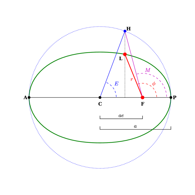
Equation (1) appears simple, but significant complication is hidden in $\phi(t)$: it varies in time in a complicated manner, and depends nonlinearly on three of the orbital parameters. In fact, no simple, direct formula for $\phi(t)$ is known; it may be calculated implicitly using two other angular coordinates for the orbital position. First is the mean anomaly, ${\cal M}$, another angle with vertex at the focus, but measuring the planet’s position projected (orthogonal to the semi-major axis) on a circle circumscribing the orbital ellipse. Figure 1 displays this peculiar construction, which makes ${\cal M}(t)$ express Kepler’s second law by varying uniformly in time: ${\cal M}(t)=2\pi t/\tau+{\cal M}_{0}$, where ${\cal M}_{0}$ is the mean anomaly at epoch $t=0$, a free parameter. Second is the eccentric anomaly, $E$, an angle defined like ${\cal M}$, but using the center of the ellipse as the vertex; it is also shown in the figure. The mean and eccentric anomalies are related via a famous transcendental equation, Kepler’s equation:

$$E-e\sin E={\cal M}.$$ (2)

Once $E$ is found from ${\cal M}$ (at a particular time of interest), $\phi$ is given by

$$\tan{\phi\over 2}=\left(1+e\over 1-e\right)^{1/2}\tan{E\over 2}.$$ (3)

The time dependence of the true anomaly thus depends on $\tau$, $e$, and ${\cal M}_{0}$.

To estimate the radial velocity of a star at a given epoch, astronomers make high-resolution measurements of the star’s spectrum, with instrumentation that imposes a number of calibration lines on the spectrum. Multiple spectra, spaced closely in time, may be taken to facilitate averaging to reduce uncertainties. A complicated joint analysis of all lines (stellar and calibration) in all spectra yields an estimate of the stellar line Doppler shift, with uncertainty summarized by a standard deviation; the uncertainty typically corresponds to a line shift of a tiny fraction of the width of a spectral pixel, corresponding to velocities of 1–10 m s^-1. But there is an additional source of velocity uncertainty. Stellar surfaces are in constant turbulent motion at high velocities. Stars are not spatially resolved in RV observations, so the measured velocity is an average over the stellar surface (and over the short time span of a single epoch’s observations). Most of the turbulent motion gets averaged away, but a small, random stellar jitter component remains, with a standard deviation, $s$, that varies from star to star and that is typically a few m s^-1 (see Wright 2005 for a compilation of jitter measurements for apparently planet-free stars). Further, stars rotate; if starspots are present, effectively masking part of the stellar surface, a small part of the rotational motion—“starspot jitter”—will contribute to the RV measurement (Makarov et al. 2009).

An RV data set is thus comprised of a set of $N$ velocity estimates and associated uncertainties, $\{v_{i},\sigma_{i}\}$, at times $t_{i}$ (not regularly spaced), where the measurements may be modeled as the sum of the systemic and Keplerian stellar velocity, and instrumental and jitter noise. We describe the uncertainty in both noise contributions with normal probability distributions. The resulting likelihood function is,

$$\mathcal{L}(\mathcal{O},\gamma,s)=\left[\prod_{i=1}^{N}\frac{1}{2\pi\sqrt{\sigma_{i}^{2}+s^{2}}}\right]\exp\left[-\frac{1}{2}\chi^{2}(\mathcal{O},\gamma,s)\right]$$ (4)

where the quantity in the exponent is the familiar goodness-of-fit statistic,

$$\chi^{2}(\mathcal{O},\gamma,s)\equiv\sum_{i}\frac{[d_{i}-v(t_{i};\mathcal{O},\gamma)]^{2}}{\sigma_{i}^{2}+s^{2}}.$$ (5)

Here $\mathcal{O}$ denotes the five orbital parameters $(K,\tau,e,\omega,{\cal M}_{0})$ that specify the Keplerian contribution to the velocity curve, $v(t)$. When we consider multiple-planet models (in Section 4), a separate set of $\mathcal{O}$ parameters appears for each planet, but there is only one $\gamma$ and one $s$ per system.

Conventional analyses of RV data first use a Lomb-Scargle periodogram (LSP; Black & Scargle 1982) to identify candidate periods, and then use a nonlinear minimizer to find a best-fit orbit by minimizing equation (5). Jitter is not handled as a free parameter ($\chi^{2}$ minimization cannot be used to estimate such variance parameters); instead, the instrumental uncertainties are scaled to make the minimum $\chi^{2}$ equal to the number of degrees of freedom (i.e., reduced $\chi^{2}$ of unity), with the excess variance attributed to jitter. Uncertainties are typically estimated either via the observed Fisher information matrix (whose inverse is asymptotically a covariance matrix estimate under regularity conditions), or using Wilks’s theorem to select $\chi^{2}$ contours (which bound confidence regions of specified asymptotic coverage under regularity conditions).

There are several shortcomings of such conventional procedures. The likelihood function is always highly multimodal, and due in part to the relative sparsity of RV data sets, there are often multiple viable modes. Also, the best-fit parameters often lie on or near parameter space boundaries (especially for $e$). These features violate the regularity conditions for use of the Fisher information or Wilks’s theorem; the resulting confidence regions can have grossly incorrect coverage. Quantities of key astrophysical interest, including the semimajor axis and the planet mass, are nonlinear functions of the parameters in the velocity model; propagating the uncertainties into such lower-dimensional nonlinear spaces is nontrivial. Uncertainty propagation into predictions (for future observations) and population-level analyses is similarly challenging. Also, there is no good way to incorporate prior information into the analysis, in particular, prior information on the scale of jitter. Finally, the LSP is closely related to least-squares fitting of a sinusoid to the data. It is not optimal for identifying candidate orbits of non-negligible eccentricity (in which case the velocity curve can be very non-sinusoidal).

Bayesian methods can address these shortcomings. Multiplying the likelihood function by a prior density, $\pi(\mathcal{O},\gamma,s)$, and normalizing, produces a posterior density in parameter space, $p(\mathcal{O},\gamma,s|D)$, with $D$ denoting the data. From a set of samples of $(\mathcal{O},\gamma,s)$ drawn randomly from the posterior, one can straightforwardly address a wide variety of inference tasks without relying on unjustifiable asymptotic approximations. Manipulation of the posterior can produce a periodogram-like quantity that improves sensitivity to eccentric orbit signals over the LSP. Some Bayesian inferences may depend on the choice of prior when the data are particularly sparse. But this dependence is useful: once data sets from many systems are available, population properties can be learned via the dependence of system inferences on the prior; this is called hierarchical or multi-level Bayesian modeling. Thus for initial system-by-system inference, we adopt interim priors, motivated in part by approximate population properties, and by convenience. Once enough systems have been discovered and analyzed, joint analysis of many interim inferences can be used to learn the system-level prior.

During the 2006 Astrostatistics Program hosted by the Statistical and Mathematical Sciences Institute (SAMSI), astronomers working on Bayesian methods for exoplanet science (including our team) settled on “default” interim priors for RV model parameters. They are motivated by basic physical constraints and approximate population-level knowledge, but attempt to be otherwise relatively uninformative (e.g., approximately flat or log-flat, but bounded where necessary to be proper). See Ford & Gregory (2007) for details. When it is useful, in our work we sometimes modify default priors, e.g., using a slightly different $K$ prior to facilitate analytic dimensional reduction. Our current completed calculations use an uninformative jitter prior for comparison with previous work, but we are also performing calculations with an informative jitter prior (based on the jitter study of Wright 2005). This can be important for obtaining realistic Bayes factors comparing models with different numbers of planets (including no planet); without an informative jitter prior, evidence for a planet can be masked when a noninformative prior allows significant residuals to be interpreted as jitter.

Before developing algorithms to implement the required calculations, it is important to understand the structure of the likelihood function. The first thing to note is that the velocity signal model, equation (1), is a linear model with respect to two parameters, $K$ and $\gamma$. Combined with the Gaussian form of the likelihood function, this implies that the dependence of the likelihood function with respect to $K$ and $\gamma$ is multivariate normal, provided other parameters are held fixed. If the prior for the linear parameters is approximately flat or normal, any needed integrals with respect to these parameters may be performed analytically (the result can be cast in terms of well-known weighted linear least squares solutions).

In fact, a simple reparameterization can reduce the nonlinear dimensionality further. Let $A_{0}=\gamma$, $A_{1}=K\cos\omega$, and $A_{2}=-K\sin\omega$. Then the velocity equation may be written as

$$v(t)=A_{0}+A_{1}[e+\cos\phi(t)]+A_{2}\sin\phi(t).$$ (6)

A single-planet model now has three linear parameters, $A\equiv(A_{0},A_{1},A_{2})$, three nonlinear orbital parameters, $\theta\equiv(\tau,e,{\cal M}_{0})$, and the jitter parameter. If we adopt a flat or normal interim prior on $A$, we can analytically marginalize over the amplitudes, effecting a significant dimensional reduction. (A flat amplitude prior corresponds to a prior that rises linearly with $K$; if desired, this can be adjusted to another prior later in the calculation via importance resampling.)

The likelihood function has relatively simple behavior with respect to $A$. To gain insight into its behavior as a function of the nonlinear parameters, Figure 2 displays slices of the amplitude-marginalized log-likelihood function along the $\tau$, $e$, and ${\cal M}_{0}$ dimensions, based on 24 RV observations of the single-planet system HD 222582 obtained over a 683 d time span with instrumentation at the Keck observatory (Vogt et al. 2000; V00). The likelihood function is highly multimodal with respect to $\tau$, relatively smooth with respect to $e$ (but for many datasets peaking on or near a boundary), and multimodal with respect to ${\cal M}_{0}$. Computational algorithms must be capable of handling these complications.

Figure 2: “Slices” of the marginal likelihood function, $\mathcal{L}_{m}(\tau,e,{\cal M}_{0})$, for orbital parameters of a single-planet model for 24 RV observations of HD 222582.

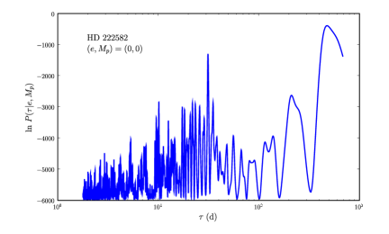
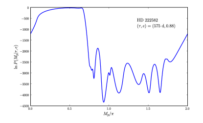
Readers familiar with periodogram methods for time series analysis will recognize the structure exhibited in the $\tau$ slice in Figure 2. In fact, for $e=0$ (in which case ${\cal M}_{0}$ is nonidentifiable), the logarithm of the marginal likelihood function for $\tau$ is proportional to the LSP to a good approximation (this follows from results in Bretthorst 2001). Accordingly, we interpret the log marginal likelihood function for nonlinear parameters, $L_{m}(\tau,e,{\cal M}_{0})$ (possibly including jitter when important), as a generalization of the LSP; we dub it a Keplerogram or K-gram. If we numerically integrate the marginal likelihood over $e$ and ${\cal M}_{0}$ (weighted by a flat prior), its logarithm offers a 1-D summary of the evidence for a planet as a function of candidate period. We dub this a Kepler periodogram.

3 Orbital Parameter Estimation and Adaptive Scheduling

The pipeline we currently use for orbital parameter estimation takes advantage of dimensional reduction to facilitate adaptive posterior sampling for exploring exoplanet models. We calculate the marginal likelihood function for the nonlinear parameters, i.e., the exponential of the Keplerogram, and posterior sampling is done in the reduced-dimension nonlinear parameter space. Once samples are available, they can be readily augmented to the full dimensional space (i.e., with amplitude parameter samples added) by drawing samples from the conditional multivariate normal distribution for $A$ given the nonlinear parameters. If we wish to adjust the interim prior, importance weights may be assigned to the samples at this step. The samples are then used for subsequent inferences.

To initialize a posterior sampler, we fix the jitter to a trial value, and explore the $(\tau,e,{\cal M}_{0})$ dependence of the marginal posterior via an adaptive grid in $\tau$ (refining the grid in regions of high posterior density), supplemented by a crude grid or quadrature in $(e,{\cal M}_{0})$ in promising $\tau$ regions. We use this exploration to build a simple, approximate $(\tau,e,{\cal M}_{0})$ sampler, used for drawing initial values for rigorous posterior sampling. For two-planet models, we follow this procedure for the first planet, and then for each member of a small set of approximate samples for the first planet’s parameters, repeat the procedure for a single-planet model for the residuals from the candidate model for the first planet. This lets us build candidate multi-Kepler models via a tractable sequence of single-planet fits. The known multiple-planet systems were first detected using such a “hieararchical” approach, in the context of the periodogram/$\chi^{2}$ minimization approach.

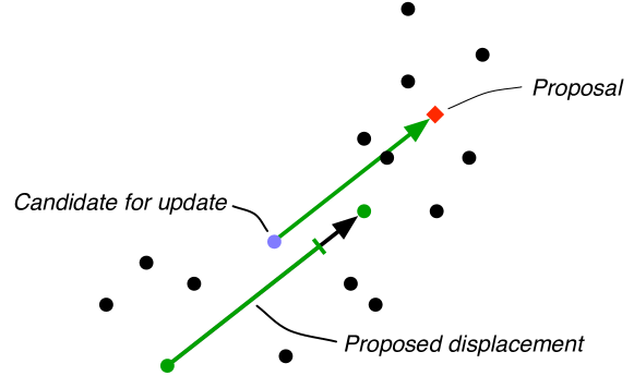
We are exploring a few different methods for posterior sampling of the marginal posterior for the nonlinear parameters. A particularly promising and simple method we are using is ter Braak’s differential evolution Markov chain (DEMC) method (ter Braak 2006). This is a population-based adaptive MCMC algorithm that weds ideas from evolutionary computing and MCMC. It evolves several chains of samples in the nonlinear parameter space, all of them targeting the marginal posterior density (in contrast to the better-known parallel tempering algorithm, where all chains but one explore annealed versions of the posterior, producing samples that are not useful in final inferences). The chains interact at every step in a way that preserves fair and asymptotically independent sampling in each chain; but the interaction effectively tunes the size and shape of the proposal distribution to match features of the target. Figures 3 depicts one DEMC update step. The algorithm enables exploration of multiple modes by different chains (partly via hopping between modes for each chain) provided the initial population includes samples from the important modes. We attempt to ensure this by building the initial population using the K-gram. The aim of the algorithm is to use a small-sized population to define adaptive Metropolis-Hastings proposals for updating each chain, with the final output being the samples in all chains.

Figure 3: Illustration of the differential evolution MCMC algorithm. Filled circles show 15 points comprising an evolving population in a two-dimensional parameter space. Blue circle indicates a point chosen at random from the 15 for possible updating. Green circles indicate pair of points chosen at random from the 14 remaining points; these determine a proposal displacement, defined as a fraction of the displacement between them. Red diamond indicates the proposed update to the blue point, found using the scaled displacement. It will be accepted or rejected via the Metropolis-Hastings rule.

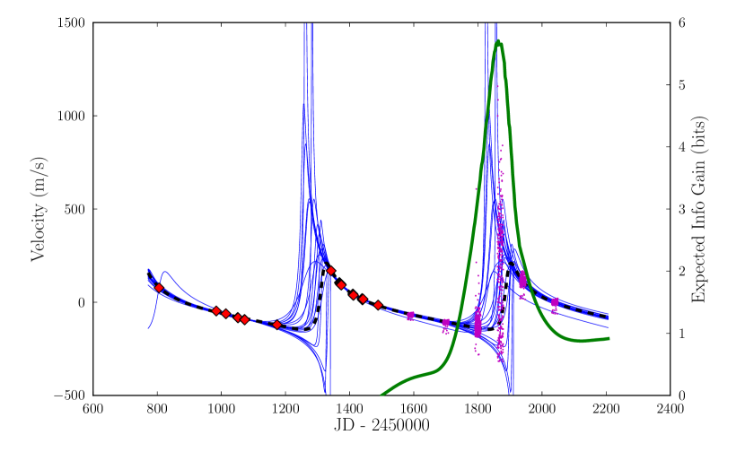
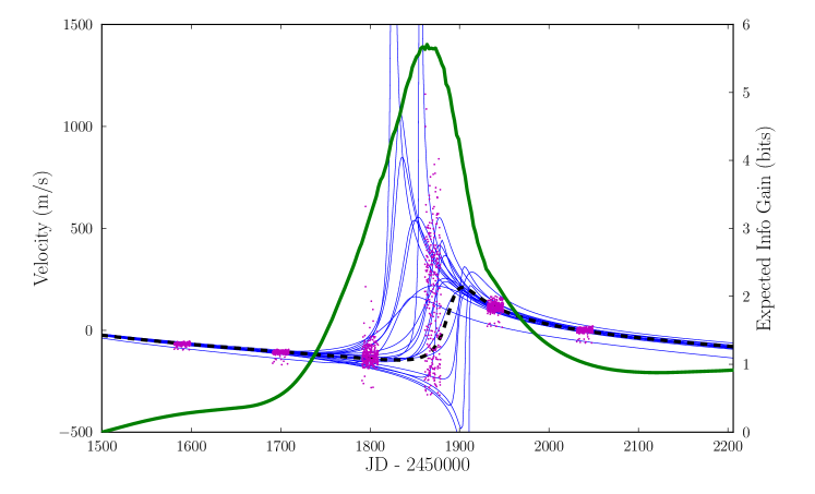
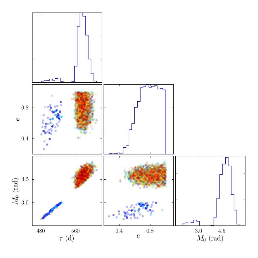
Figures 4 and 5 show selected results from this approach, for a single-planet model for the 24 Keck RV observations from HD 222582. Figure 4 (top panel) shows the data as (red) diamonds, at times earlier than $\sim 1400$ d (the $\approx$ 3 m s^-1 error bars are smaller than the symbols). The dashed black curve shows the best-fit orbit reported by V00, with a period of 579.5 d and a high eccentricity, $e=0.71$. We used our pipeline to initialize and evolve a population of 10 chains for 20,000 steps; convergence and mixing were assessed via the Gelman-Rubin $R$ statistic (readily calculated from DEMC parallel chains) and by inspection of trace plots and autocorrelation functions. The thin blue curves show the velocity curves for 20 models chosen at random from the posterior samples (after thinning by a factor of ten). A wide variety of orbits are consistent with the data; no single orbit fairly represents the possibilities (in fact, the best-fit orbit seems not very representative). Figure 5 shows pairwise scatterplots and marginal histograms (along the diagonal) of the posterior samples for the nonlinear orbital parameters, summarizing the parameter uncertainties. Sample points are transparently colored, indicating time in the Markov chain; blue points are early in the chain, green and yellow points at intermediate times, and orange and red points at late times. For this analysis the initial population was drawn from the marginal distribution with $e=0$; its logarithm is essentially the LSP. The separation of the blue “cool” points from later points shows that the period for the peak of the LSP was in the general vicinity of the global mode but did not accurately locate it; all chains soon leave the vicinity of the initial population (this burn-in phase of the chain would normally be discarded for final inferences; we have kept it in this figure for illustration, but discarded burn-in samples in later figures). The DEMC algorithm is able to adapt to the posterior and find and explore the local mode in a few thousand iterations (the burn-in time shortens to a few hundred steps with a more sophisticated initialization using the full K-gram).

Figure 4: Results from single-planet modeling of 24 RV observations of HD 222582 reported in V00 (as revised in B06). Shown are observations (red diamonds, several overlapping), best-fit velocity model (thick dashed black curve), 20 representative models from posterior (thin blue curves), 300 samples from predictive distribution for velocity at six epochs (magenta points), and relative expected information gain vs. future observing time (green curve, right axis). Time is barycentric Julian day relative to 2,450,000. Bottom panel expands the later half of the plot.

Figure 5: Parameter estimation results from single-planet modeling of 24 RV observations of HD 222582 reported in V00. Shown are pairwise scatter plots and marginal histograms (along the diagonal) for $\tau$, $e$, ${\cal M}_{0}$; color indicates time in Markov chain (early to late in spectral sequence from blue to red).

Posterior samples enable straightforward propagation of uncertainties into nontrivial inferences. For example, we can easily create samples from the (marginal) posterior distribution for the physically important derived parameters $a$ and $m_{p}\sin i$ (where $i$ is the inclination of the orbital plane to the plane of the sky; $m_{p}$ and $i$ are not separately identifiable in models for RV data) by evaluating them for each posterior sample. They also enable us to tackle problems requiring prediction under uncertainty, including adaptive scheduling of future observations (LC00, LC04, L04). From available data, $D$, we can calculate a posterior predictive distribution for the value of a future datum at time $t$, $d_{t}$;

$$p(d_{t}|D)=\int p(\mathcal{P}|D)\,p(d_{t}|\mathcal{P})\,d\mathcal{P},$$ (7)

where $\mathcal{P}$ denotes all of the parameters in the currently considered model. The first factor in the integrand is the posterior distribution for $\mathcal{P}$. The second factor is the probability for a future measured value, given values for the parameters; this is just a normal distribution centered at the predicted velocity. The predictive distribution can be easily evaluated or sampled from using posterior samples.

To optimally schedule a new observation, we must specify some measure of the value a new observation would have for our observational goals; this is the utility function in the decision-theoretical formulation of adaptive scheduling, described in LC03. For a general-purpose measure of the value of new data for a variety of goals, we appeal to information theory: we seek new data that will make the updated posterior most informative about the parameters, i.e., leading to the largest expected decrease in the uncertainty, quantified by Shannon entropy (or, equivalently here, by Kullback-Leibler divergence). A straightforward calculation shows that the posterior uncertainty is expected to decrease the most if we observe at the time for which the predictive uncertainty—the entropy of $p(d_{t}|D)$—is greatest: we learn the most by sampling where we know the least. This is called maximum entropy sampling (Sebastiani & Wynn 2000).

We use posterior samples to calculate a straightforward Monte Carlo estimate of the entropy in the predictive distribution as a function of time, $S(t)$. The green curve in Figure 4 (expanded in the bottom panel) shows $S(t)$ for times spanning about one orbit following the observations reported in V00, in units of bits of information gain, relative to the information that would be gained by repeating the last observation (one bit of information roughly corresponds to reducing the volume of a joint credible region by one half, a very significant information gain). $S(t)$ essentially measures the vertical spread of the predicted velocity curves at time $t$. To reveal more detail in the predictive distribution as a function of time, we show (magenta) point clouds of samples of $d_{t}$ from $p(d_{t}|D)$ at six different times (the times are dithered over an interval of $\pm 5$ d to spread the points). The points reveal the predictive distribution to be complicated, especially in regions of high uncertainty. It can be highly skew and even multimodal; clearly the predictive uncertainties would not be well-described by normal distributions (which underlie classical experimental design theory). The entropy curve shows that observations at the optimal time ($t\approx 1870$ d) are much more informative than observations even a small fraction of a period earlier or later.

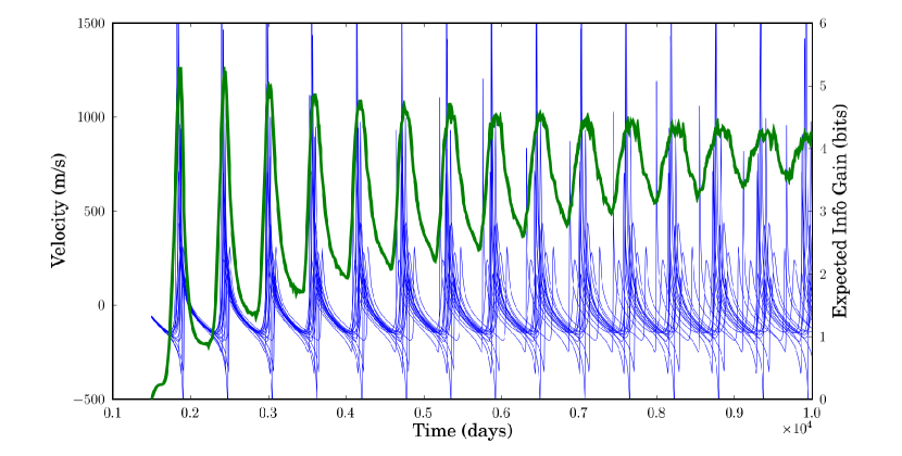
Figure 6 is a similar plot, but extending the $S(t)$ curve further into the future, over about 14 orbits. It shows that the most information will be gained by following up the initial observations within the time of the subsequent orbit or two. There are definitely preferred times in later orbits, but the maximum expected information gain is decreasing, and the maximum and minimum of the expected information gain are converging. These features are in accord with intuition: the significant uncertainties in the orbital period and shape imply that our ability to predict decreases with time, until after many orbits we cannot even confidently predict the number of orbits that have passed. At late times, our predictions become so poor that no candidate observing time is clearly preferable to another.

Figure 6: Relative expected information gain for a single future observation of HD 222582, for times $\approx 14$ orbits after original observations (green curve, right axis), with 15 representative velocity models (thin blue curves).

We would like to see how adaptive scheduling can improve results compared to non-optimal scheduling. LC03 and L04 reported results of a few simulations demonstrating the superiority of adaptive scheduling to informal or random sampling. Ford (2008) performed a more extensive simulation study, focusing on the significantly simpler case of circular orbits, even more convincingly demonstrating the benefits of the approach, though still with simulated data.

A more convincing demonstration would use real data, for example, comparing results from subsequent observing of HD 222582 with an optimized schedule to results from a non-optimized schedule. Butler et al. (2006; B06) reported 13 subsequent observations, at times not chosen to optimize information gain. Figure 7 is similar to Figure 4, but extending the $S(t)$ curve farther in the future, over about 4 orbits, covering the span of the new observations of B06. While a few observations were not far from a local optimum, many observations were at times offering much less expected information gain than optimal times. To see what might have been gained with optimal observing, we simulate a new observation at the first (global) optimal time, update interim inferences, calculate a new entropy curve, and repeat for a few cycles. We do not know the true orbit of HD 222582 to use for the simulations; as a reasonable surrogate, we use the best-fit orbit reported by B06 using all 37 observations.

Figure 7: Relative expected information gain for a single future observation of HD 222582 for times $\approx 4$ orbits after after the observations of V00 (thick green curve, right axis), with 20 representative velocity models (thin blue curves, left axis). Red diamonds indicated the the subsequent 13 observations of B06, at times indicated by vertical dashed red lines.

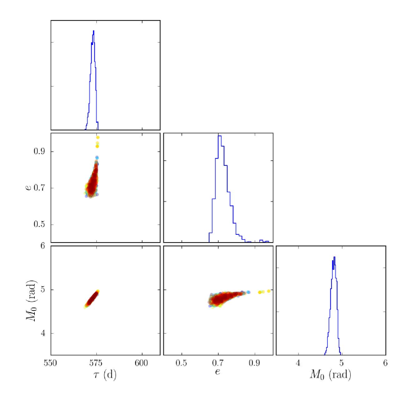
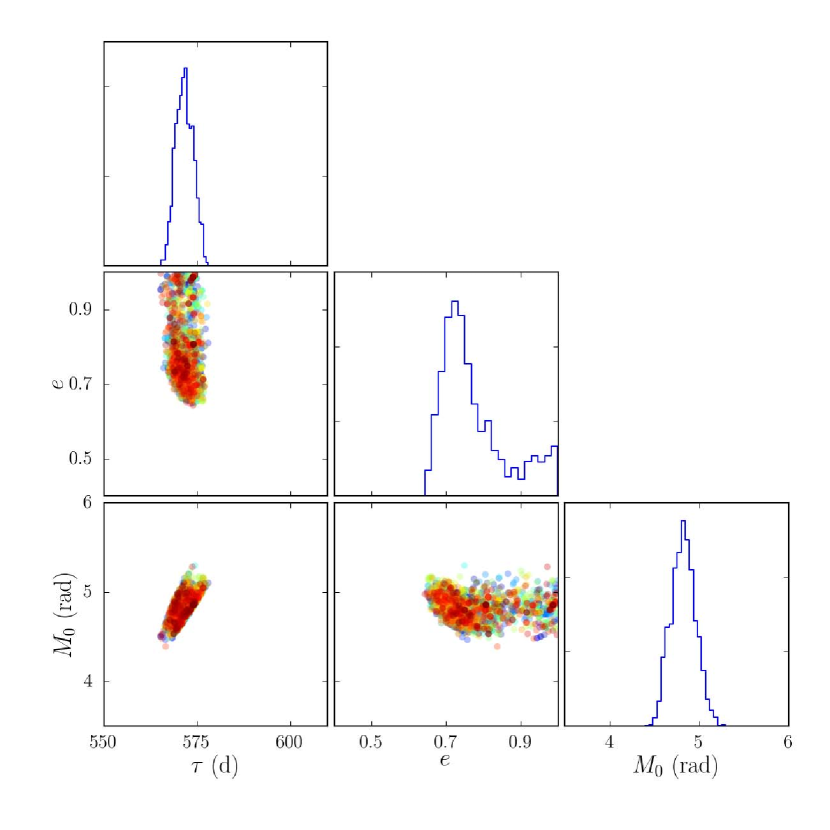
Figures 8 and 9 show posterior samples summarizing inferences with new data. Figure 8 shows results from using the 24 V00 observations and adding just three new, optimal observations (for 27 total observations). Figure 9 shows results adding all 13 non-optimal observations from B06 instead of the three optimal observations (for 37 total observations). The posterior distribution based on three new optimal observations is dramatically more precise than the initial interim posterior (displayed in Figure 5), and is also much more precise than the posterior based on 13 non-optimal observations (and it is converging on the surrogate “true” parameter values). This clearly demonstrates the potential of adaptive observing for improving orbital parameter estimates. We are performing similar calculations for other heavily-observed systems to more fully assess the benefits of the approach.

Figure 8: Orbital parameter posterior samples for HD 222582 based on 24 early observations and three simulated new observations at optimal times.

Figure 9: Orbital parameter posterior samples for HD 222582 based on 24 early and 13 new, non-optimal actual observations (bottom).

4 Planet Detection Via Model Comparison

To detect a planet, we must compare hypotheses with no planet (i.e, with just $\gamma$ and $s$ parameters), to hypotheses specifying a single planet. The comparison must account for the fact that both the no-planet and single-planet models are composite; we do not know the best (or true) parameter values a priori, and they remain uncertain (albeit less so) even after fitting the best data sets. To detect additional planets, we must similarly compare multi-Kepler models to the single-planet model. To optimally schedule observations for planet detection (as opposed to orbit estimation, treated above), we must incorporate model uncertainty into prediction and experimental design calculations.

In Bayesian parameter estimation, the data influence inferences via the likelihood function, the probability for the data considered as a function of the parameters specifying a simple (point) hypothesis for the data. For comparing rival parametric models, Bayes’s theorem similarly indicates that the data influence model choice through a likelihood—i.e., a probability for the data given a hypothesis—but now the likelihood is for a hypothesis specifying a model as a whole, i.e., a composite hypothesis. This quantity may fairly be called simply the likelihood for a model (as a whole); more conventionally it is called the marginal likelihood, referring to how it is calculated from the likelihood function for the model’s parameters (and helping to distinguish it linguistically from the likelihood function). The marginal likelihood is the integral of the product of a model’s prior and likelihood, over the entire parameter space. Such integrals are often challenging if the dimension of the parameter space is greater than a few.

For RV data, the no-planet model is only two-dimensional, and the marginal likelihood integral over $(\gamma,s)$ is easy to calculate. Already for the single-planet model, the parameter space is seven-dimensional and the likelihood is highly structured; direct numerical cubature over all seven dimensions is challenging. If we are willing to adopt interim priors allowing analytical amplitude marginalization, numerical cubature is needed only over the three-dimensional nonlinear parameter space (with a fourth dimension added when jitter uncertainty is important). This is tractable via cubature. But adding a second or third planet makes marginal likelihood calculation via cubature intractable.

The marginal likelihood needed for model comparison is just the normalization constant for the posterior distribution used for parameter estimation. We can sample the posterior distributions for multi-planet models with the approach of Section 3. But the normalization constant does not appear (and is not needed) in MCMC algorithms, so this ability does not directly help us (although there are indirect ways to use MCMC output to estimate marginal likelihoods; see Clyde et al. 2007).

We have developed a new method for estimating marginal likelihoods, based on marrying ideas from adaptive importance sampling, mixture models, and sequential Monte Carlo (SMC) methods. At present we have implemented it as a general-purpose ab-initio algorithm, without taking advantage of any analytical marginalization or results from MCMC-based posterior exploration. Denote the full parameter space as $\mathcal{P}$, and let $q(\mathcal{P})=\pi(\mathcal{P})\mathcal{L}(\mathcal{P})$; the marginal likelihood is $Z=\int q(\mathcal{P})d\mathcal{P}$. Suppose we could construct an importance sampling density, $Q(\mathcal{P})$, that resembles the target, $q(\mathcal{P})$, but that we could cheaply sample from and evaluate. Then we could easily get accurate $Z$ estimates via the usual importance sampling algorithm. The problem is that it is difficult to construct such importance samplers (see, e.g., Oh & Berger 1993, West 1993).

Instead of attempting to build an efficient importance density $Q(\mathcal{P})$ ab initio, we build a sequence of samplers, $Q_{n}(\mathcal{P})$, approximating annealed versions of the target, starting with a nearly flattened target, and ending with the actual target. Each sampler is built using a mixture of multivariate Student-$t$ distributions with $M$ components (setting the degrees of freedom to a small value such as 5). The number $M$, the component weights, and the locations and scale matrices for each component are calculated using samples from the previous step’s sampler. In outline, we start with a dispersed importance density, $Q_{0}(\mathcal{P})$, and we set the initial annealed target density, $q_{0}(\mathcal{P})$, equal to $Q_{0}$. The algorithm then cycles through the following steps (starting with $n=1$) until an acceptably small importance sampling variance is achieved:

1. Anneal the target from $q_{n-1}$ to $q_{n}=Q_{0}^{1-\beta_{n}}q^{\beta_{n}}$, where $\beta_{n}$ is a sequence of “inverse temperatures” increasing from 0 to 1 according to an annealing schedule (we use both standard rules of thumb for the schedule and adaptive schedules; in our examples they worked equally well).

2. Sample parameter values $\{\mathcal{P}_{i}\}$ from $Q_{n-1}$; assign them weights $w_{i}=q_{n}(\mathcal{P}_{i})/Q_{n-1}(\mathcal{P}_{i})$.

3. Refine $Q_{n-1}$ to $Q_{n}$, intended to approximate $q_{n}$:

   1. Revise the Student-$t$ component parameters and mixture weights using the Expectation-Maximization (EM) algorithm to minimize the Kullback-Leibler divergence between $Q_{n}$ and $q_{n}$, estimated using the samples and sample weights.

   2. Delete mixture components with small mixture weights.

   3. Merge components that have large mutual information.

   4. Split components with large weights by duplicating them, revising their parameters via the EM algorithm, and keeping the split if the mutual information between the revised components is low.

The final sampler can be used to estimate $Z$, and the importance-weighted samples can be used for parameter estimation; the algorithm thus may be able to replace our K-gram/DEMC parameter estimation pipeline in certain settings. We call the algorithm annealing adaptive importance sampling (AAIS). Liu et al. (2011; L11) provides a detailed description; here we highlight some illustrative results.

Figure 10 shows AAIS in operation on a highly multimodal two-dimensional target with known marginal likelihood. The target consists of a mixture of 10 bivariate normals, all well-separated and with very different covariance matrices. The initial importance sampler, $Q_{0}(\mathcal{P})$, is a set of 10 bivariate $t$ distributions spread randomly across the space; it is illustrated by the contours and crosses in the left panel. The annealing schedule has $\beta_{n}$ varying from 0.01 to 1 for $n=1$ to 8. We draw samples (red dots) from $Q_{0}$, intended to approximate $q_{0}$; anneal the target to $q_{1}$; use $q_{1}$ to weight the samples; and then use the weighted samples to adjust $Q_{0}$ to a new sampler, $Q_{1}$, intended to approximate $q_{1}$, as outlined above. The middle panel shows the third step ($\beta_{3}=0.11$), revealing that $Q_{2}$ is capturing the features of the annealing target. The right panel shows that in eight steps all modes are located and well-modeled. The final importance sampler, $Q_{8}$, has an efficiency of 94%, and estimates $Z$ to 0.25% accuracy with 2000 samples (the accuracy estimate is from the usual importance sampling variance).

Figure 10: Three stages of the AAIS algorithm in operation on a mixture of 10 well-separated bivariate normals with differing scales and correlations. From left to right, the annealed target has a temper of $\beta_{n}=0.01$, 0.11, and 1, corresponding to steps $n=1$, 3, and 8.

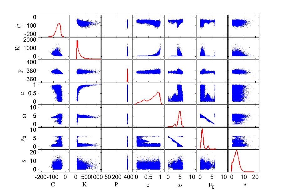
Figure 11 shows AAIS results from a two-planet fit to 30 RV observations of HD 73526, a system known to contain two planets with orbital periods of 188 d and 377 d (Tinney et al. 2006). The panel shows parameter estimates for the orbit of the second (longer-period) planet; the sampling efficiency of the final sampler is $\approx 65$%; similar or higher efficiencies were obtained for single-planet and no-planet models. The Bayes factor (ratio of marginal likelihoods) for the single-planet model vs. the no-planet model is $6.5\times 10^{6}$ ($\pm 3$%); for two-planet vs. one-planet it is $8.2\times 10^{4}$ ($\pm 4$%); this indicates very strong evidence for two planets around HD 73526. To provide confidence in the estimates and uncertainties, we have validated AAIS by applying it to a variety of multivariate test integrands more complicated than the illustrative two-dimensional case above, including integrands designed to mimic key features of RV likelihood functions; L11 describes some of these cases.

Figure 11: AAIS parameter estimates from an analysis of data from HD 73526; shown are pairwise scatterplots and marginal histograms (curves, along the diagonal) for the orbital parameters of the longer-period planet in a two-planet model. Renamed parameters (following L11) are: $P=\tau$, $C=\gamma$, $\mu_{0}={\cal M}_{0}$.

We are continuing to refine our K-gram/DEMC pipeline and the AAIS algorithm. We are exploring how the algorithms compare for parameter estimation, and how the K-gram may be used to accelerate the AAIS algorithm (via dimensional reduction and a “smart start”). Our main longer-term goal is to generalize the adaptive scheduling approach described in Section 3 for orbit estimation, instead optimizing the timing of future observations for both planet detection and orbit estimation simultaneously. This requires incorporating AAIS in the calculation (to handle planet number uncertainty), and considering non-greedy, multiple-step scheduling designs.

Acknowledgments: We are grateful to two referees whose comments helped improve the manuscript, and to the editors for relaxing page constraints to allow us to address the referees’ questions. Work reported here was funded in part by NSF grants DMS-042240, AST-0507481, and AST-0507589, and by the NASA Space Interferometry Mission via JPL subcontracts and the SIM Science Studies program.

References

- Balan and Lahav [2009] S.T. Balan, O. Lahav, EXOFIT: Orbital parameters of extrasolar planets from radial velocities, Mon. Not. Roy. Astron. Soc. 394 (2009) 1936–1944.
- Black and Scargle [1982] D.C. Black, J.D. Scargle, On the detection of other planetary systems by astrometric techniques, Astrophys. J. 263 (1982) 854–869.
- Bretthorst [2001] G.L. Bretthorst, Generalizing the Lomb-Scargle periodogram, in: A. Mohammad-Djafari (Ed.), Bayesian Inference and Maximum Entropy Methods in Science and Engineering, volume 568 of American Institute of Physics Conference Series, 2001, pp. 241–245.
- Butler et al. [2006] R.P. Butler, J.T. Wright, G.W. Marcy, D.A. Fischer, S.S. Vogt, C.G. Tinney, H.R.A. Jones, B.D. Carter, J.A. Johnson, C. McCarthy, A.J. Penny, Catalog of nearby exoplanets, Astrophys. J. 646 (2006) 505–522.
- Chib and Jeliazkov [2001] S. Chib, I. Jeliazkov, Marginal likelihood from the Metropolis-Hastings output, J. Amer. Statist. Assoc. 96 (2001) 270–281.
- Clyde et al. [2007] M.A. Clyde, J.O. Berger, F. Bullard, E.B. Ford, W.H. Jefferys, R. Luo, R. Paulo, T. Loredo, Current challenges in Bayesian model choice, in: G. J. Babu & E. D. Feigelson (Ed.), Statistical Challenges in Modern Astronomy IV, volume 371 of Astronomical Society of the Pacific Conference Series, 2007, p. 224.
- Cumming [2004] A. Cumming, Detectability of extrasolar planets in radial velocity surveys, Mon. Not. Roy. Astron. Soc. 354 (2004) 1165–1176.
- Cumming and Dragomir [2010] A. Cumming, D. Dragomir, An integrated analysis of radial velocities in planet searches, Mon. Not. Roy. Astron. Soc. 401 (2010) 1029–1042.
- Ford [2005] E.B. Ford, Quantifying the uncertainty in the orbits of extrasolar planets, Astronom. J. 129 (2005) 1706–1717.
- Ford [2008] E.B. Ford, Adaptive scheduling algorithms for planet searches, Astronom. J. 135 (2008) 1008–1020.
- Ford and Gregory [2007] E.B. Ford, P.C. Gregory, Bayesian model selection and extrasolar planet detection, in: G. J. Babu & E. D. Feigelson (Ed.), Statistical Challenges in Modern Astronomy IV, volume 371 of Astronomical Society of the Pacific Conference Series, 2007, pp. 189–206.
- Gregory [2005] P.C. Gregory, A Bayesian analysis of extrasolar planet data for HD 73526, Astrophys. J. 631 (2005) 1198–1214.
- Gregory [2011] P.C. Gregory, Bayesian exoplanet tests of a new method for MCMC sampling in highly correlated model parameter spaces, Mon. Not. Roy. Astron. Soc. 410 (2011) 94–110.
- Haario et al. [2001] H. Haario, E. Saksman, J. Tamminen, An adaptive Metropolis algorithm, Bernoulli 7 (2001) 223–242.
- Liu et al. [2010] B. Liu, J. Berger, M.A. Clyde, J.I. Crooks, T.J. Loredo, D.F. Chernoff, Adaptive annealed importance sampling for multi-modal posterior exploration and model selection with application to extrasolar planet detection (2010) (in preparation).
- Loredo [2004] T.J. Loredo, Bayesian adaptive exploration, in: G. J. Erickson & Y. Zhai (Ed.), Bayesian Inference and Maximum Entropy Methods in Science and Engineering, volume 707 of American Institute of Physics Conference Series, 2004, pp. 330–346.
- Loredo and Chernoff [2000] T.J. Loredo, D.F. Chernoff, Bayesian methodology for the Space Interferometry Mission, in: Bulletin of the American Astronomical Society, volume 32 of Bulletin of the American Astronomical Society, 2000, p. 767.
- Loredo and Chernoff [2003] T.J. Loredo, D.F. Chernoff, Bayesian adaptive exploration, in: Feigelson, E. D. & Babu, G. J. (Ed.), Statistical Challenges in Astronomy, Springer, 2003, pp. 57–70.
- Makarov et al. [2009] V.V. Makarov, C.A. Beichman, J.H. Catanzarite, D.A. Fischer, J. Lebreton, F. Malbet, M. Shao, Starspot jitter in photometry, astrometry, and radial velocity measurements, Astrophys. J. Lett. 707 (2009) L73–L76.
- Marcy et al. [2004] G.W. Marcy, P.R. Butler, S. Frink, D. Fischer, B. Oppenheimer, D.G. Monet, A. Quirrenbach, J.D. Scargle, Discovery of planetary systems With SIM, in: S. Unwin & S. Turyshev (Ed.), Science with the Space Interferometry Mission, 2004, pp. 3–6 (collection of SIM Science Team project summaries; full proposal for this project at http://sim.jpl.nasa.gov/scienceMotivations/exoplanets/).
- Oh and Berger [1993] M.S. Oh, J.O. Berger, Integration of multimodal functions by Monte Carlo importance sampling, J. Amer. Statist. Assoc. 88 (1993) 450–456.
- Sebastiani and Wynn [2000] P. Sebastiani, H.P. Wynn, Maximum entropy sampling and optimal Bayesian experimental design, Journal of the Royal Statistical Society, Series B: Statistical Methodology 62 (2000) 145–157.
- ter Braak [2006] C. ter Braak, A Markov Chain Monte Carlo version of the genetic algorithm Differential Evolution: easy Bayesian computing for real parameter spaces, Statistics and Computing 16 (2006) 239–249.
- Tinney et al. [2006] C.G. Tinney, R.P. Butler, G.W. Marcy, H.R.A. Jones, G. Laughlin, B.D. Carter, J.A. Bailey, S. O’Toole, The 2:1 resonant exoplanetary system orbiting HD 73526, Astrophys. J. 647 (2006) 594–599.
- Tuomi [2011] M. Tuomi, Bayesian re-analysis of the radial velocities of Gliese 581. Evidence in favour of only four planetary companions, Astron. & Astrophys. 528 (2011) L5+.
- Vogt et al. [2000] S.S. Vogt, G.W. Marcy, R.P. Butler, K. Apps, Six new planets from the Keck Precision Velocity Survey, Astrophys. J. 536 (2000) 902–914.
- West [1993] M. West, Approximating posterior distributions by mixtures, J. Roy. Statist. Soc. Ser. B 55 (1993) 409–422.
- Wright [2005] J.T. Wright, Radial velocity jitter in stars from the California and Carnegie Planet Search at Keck Observatory, Pub. Astron. Soc. Pac. 117 (2005) 657–664.