Gaussian state for the bouncing quantum cosmology

Abstract

We present results concerning propagation of the Gaussian state across the cosmological quantum bounce. The reduced phase space quantization of loop quantum cosmology is applied to the Friedman-Robertson-Walker universe with a free massless scalar field. Evolution of quantum moments of the canonical variables is investigated. The covariance turns out to be a monotonic function so it may be used as an evolution parameter having quantum origin. We show that for the Gaussian state the Universe is least quantum at the bounce. We propose explanation of this counter-intuitive feature using the entropy of squeezing. The obtained time dependence of entropy is in agreement with qualitative predictions based on von Neumann entropy for mixed states. We show that, for the considered Gaussian state, semiclassicality is preserved across the bounce, so there is no cosmic forgetfulness.

I Introduction

The available data of observational cosmology indicate that the Universe emerged from a state with extremely high energy densities of matter fields. Theoretical cosmology, in particular the Belinskii-Khalatnikov-Lifshitz (BKL) scenario (generic solution of general relativity devoid of any assumption on the symmetry of spacetime) predicts an existence of the initial cosmological singularity with diverging gravitational and matter fields invariants BKL1 ; BKL2 ; BKL3 . Both the observation and the theory indicate that the cosmological singularity, identified at the classical level, may have much to do with an extreme initial state in the evolution of the Universe. An existence of the general solution to the Einstein equations with the cosmological singularity means that this classical theory is incomplete. It is expected that finding the singularity free quantum BKL theory would help in the construction of a theory unifying gravitation and quantum physics, and could be used to describe the very early Universe.

The challenge of quantization of the BKL scenario should be preceded by complete understanding of quantum aspects of some special cases of this model. For instance, the Friedman-Robertson-Walker (FRW) model can be used for such a purpose OIB . In particular, an evolution of the quantum FRW model has not been fully understood yet.

Presently, quantum cosmology effects are commonly addressed within loop quantum cosmology (LQC) methods. This approach has two alternative forms: standard LQC (see, e.g., Ashtekar:2003hd ; Bojowald:2006da ; Ashtekar:2006wn ) and nonstandard LQC (see, e.g., Dzierzak:2009ip ; Malkiewicz:2009qv ; Mielczarek:2011mx ). The LQC methods rely on modifying general relativity by approximating the curvature of connection by holonomies around small loops. Such modification leads to replacing classical singularities by quantum bounces Ashtekar:2003hd ; Bojowald:2006da ; Ashtekar:2006wn ; Dzierzak:2009ip ; Malkiewicz:2009qv ; Mielczarek:2011mx .

In this paper, we apply the nonstandard LQC to the flat FRW model coupled to a free massless scalar field. The presented results are a continuation of investigations initiated in our recent paper Mielczarek:2011mx . Here, we focus on analysis of the quantum dynamic for the state being a Gaussian packet constructed by using eigenstates of a physical Hamiltonian. There are at least two reasons to consider this particular state. First, strictly analytical results can be obtained allowing detailed analysis of the model. It is advantageous to have analytical toy models for testing more sophisticated models. Second, the Gaussian packets are shown to emerge in the process of decoherence Zurek:1991vd ; Zurek:2003zz for various physical systems (see, e.g., Zurek:1992mv ; Kiefer:2006je ). Therefore, they serve as a good description of semiclassicality. The minisuperspace model of the Universe can be treated as an outcome of decoherence of the relevant degrees of freedom (as the scale factor) with respect to the irrelevant degrees of freedom (as perturbations) belonging to superspace. Thus, one can expect the minisuperspace model of the Universe in the semiclassical regime to be described by the Gaussian-type packet. Moreover, even if the obtained state is not exactly the Gaussian function, the Gaussian one serves as a reasonable approximation of any other single-peaked distribution.

The organization of the paper is as follows. In Sec. II, we introduce the quantum Hamiltonian for the considered model and study the corresponding eigenproblem, which was solved in Ref. Mielczarek:2011mx . The obtained eigenfunctions are subsequently used to construct the Gaussian packet state. In Sec. III, we study the evolution of the quantum moments of the canonical variables for the state under consideration. We focus on investigating dynamics of mean values, dispersions, and covariance. Our analysis shows that for the Gaussian packet, quantum uncertainty is minimal at the bounce. In Sec. IV, notion of quantum entropy of squeezing is introduced. Evolution of this entropy for the considered state is investigated. We show that the minimum uncertainty at the bounce is related with the state of minimum entropy. In Sec. V, relative fluctuations are studied in the context of the so-called cosmic forgetfulness. In Sec. VI, we draw conclusions and indicate further directions of investigation.

II Hamiltonian and evolution

The physical classical Hamiltonian of the system is found to be Mielczarek:2011mx

$$H_{\lambda}=\frac{2}{\lambda\sqrt{G}}P\sin(\lambda Q),$$ (1)

where $G$ is Newton’s constant. The parameter $\lambda$ of the theory may be related to the minimum area of the loop used to determine the holonomies (its precise value in the nonstandard LQC has to be fixed observationally). The variables $Q$ and $P$ may be interpreted in terms of the Hubble constant and the volume of space, respectively. They satisfy the algebra $\{Q,P\}=1$, and have the domains $\lambda Q\in[0,\pi]$ and $P>0$.

The quantum Hamiltonian corresponding to (1) reads Mielczarek:2011mx

$$\hat{H}_{\lambda}\psi=-\frac{i}{\lambda\sqrt{G}}\left(2\sin(\lambda Q)\frac{d}{dQ}+\lambda\cos(\lambda Q)\right)\psi,$$ (2)

where $\psi\in L^{2}([0,\pi/\lambda],dQ)=:\mathcal{H}$. The eigenvalue problem $\hat{H}_{\lambda}\Psi_{E}=E\Psi_{E}$ has the solution

$$\Psi_{E}(x)=\sqrt{\frac{\lambda\sqrt{G}}{4\pi}\cosh\ \left(\frac{2}{\sqrt{G}}x\right)}\;e^{iEx},~{}~{}~{}~{}E\in\mathbb{R},$$ (3)

where $x:=\frac{\sqrt{G}}{2}\ln\left|\tan\left(\frac{\lambda Q}{2}\right)\right|$. One may easily verify that $\langle\Psi_{E}|\Psi_{E^{\prime}}\rangle=\delta(E^{\prime}-E)$.

We specify the domain of the unbounded operator $\hat{H}_{\lambda}$ as follows:

$$D(\hat{H}_{\lambda}):={\rm span}\{\varphi_{k},~{}~{}k\in\mathbb{Z}\},$$ (4)

where

$$\varphi_{k}(Q):=\int_{-\infty}^{\infty}c_{k}(E)\Psi_{E}(Q)\;dE,~{}~{}~{}c_{k}\in C^{\infty}_{0}(\mathbb{R}).$$ (5)

The domain $D(\hat{H}_{\lambda})$ is a dense subspace of $\mathcal{H}$, and an action $\hat{H}_{\lambda}$ does not lead outside of $D(\hat{H}_{\lambda})$. It has been shown in Mielczarek:2011mx that $\hat{H}_{\lambda}$ is an essentially self-adjoint operator on $D(\hat{H}_{\lambda})$.

Making use of the Stone theorem RaS , we define the unitary operator of an evolution as follows:

$$\hat{U}(s):=\exp\left\{-\frac{i}{\hslash}s\hat{H}_{\lambda}\right\},$$ (6)

where $s\in\mathbb{R}$ is a “time” parameter. The state at any moment of time, conv , can be found as follows: $|\Psi(s)\rangle=\hat{U}(s)|\Psi(0)\rangle=\exp\{-is\hat{H}_{\lambda}\}|\Psi(0)\rangle$.

Let us consider a superposition of the Hamiltonian eigenstates $|\Psi(0)\rangle=\int_{-\infty}^{+\infty}dEc(E)|\Psi_{E}\rangle$ at $s=0$. Then, evolution of this state is given by

$$|\Psi(s)\rangle=\int_{-\infty}^{+\infty}dEc(E)e^{-isE}|\Psi_{E}\rangle.$$ (7)

In what follows, we consider the Gaussian packet with a simple profile,

$$c(E):=\sqrt[4]{2\alpha/\pi}\exp\left\{-\alpha(E-E_{0})^{2}\right\},$$ (8)

that is centered at $E_{0}$ with the dispersion parametrized by $\alpha$. We find that the normalized packet defined by (7) and (8) reads

$$\Psi(x,s)=\sqrt{\frac{\lambda\cosh\ \left(\frac{2}{\sqrt{G}}x\right)}{\sqrt{8\pi\tilde{\alpha}}}}e^{-\frac{(x-s)^{2}}{4\alpha}}e^{iE_{0}(x-s)},$$ (9)

where $\tilde{\alpha}:=\alpha/G$ (for further purposes, we also define $\tilde{E}_{0}:=E_{0}\sqrt{G}$).

III Quantumness

To get some insight into the nature of the quantum bounce, one studies possible correlation between quantum fluctuations before and after the bounce. In particular, one tries to find the answer to the question: Is the semiclassicality of the Universe preserved across the bounce? If the answer is negative, we would not be able to learn what had happened before the big bounce. It is called the cosmic forgetfulness or amnesia BojowaldNature ; Corichi:2007am . We will come to this problem in Sec. V.

Another issue, partially related with forgetfulness, is the quantumness of the Universe. This property can be studied by analyzing quantum moments of the canonical variables. Here, we will focus on mean values $\langle\hat{Q}\rangle$ and $\langle\hat{P}\rangle$, dispersions $\Delta\hat{Q}:=\sqrt{\langle\hat{Q}^{2}\rangle-\langle\hat{Q}\rangle^{2}}$ and $\Delta\hat{P}:=\sqrt{\langle\hat{P}^{2}\rangle-\langle\hat{P}\rangle^{2}}$, and covariance

$$C_{QP} := \langle(\hat{Q}-\langle\hat{Q}\rangle)(\hat{P}-\langle\hat{P}\rangle)\rangle$$ (10)

$$= \frac{1}{2}\langle\hat{Q}\hat{P}+\hat{P}\hat{Q}\rangle-\langle\hat{Q}\rangle\langle\hat{P}\rangle.$$

The lowest moments listed above give us the basic characteristics of a quantum state.

An important property of the quantum state (9) is that its covariance is nonvanishing. In Fig. 1, we show a representative example of $C_{QP}$ as a function of time.

Figure 1: Covariance $C_{QP}$ for $\tilde{\alpha}=0.1$ and $\tilde{E}_{0}=10$.

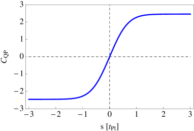
The covariance is a monotonic function of time, and it crosses zero value just at the point of bounce ($s=0$). The monotonic behavior of $C_{QP}$ suggest that covariance may serve as an internal time parameter. In such a case, the time would have purely quantum nature, different from the time parameter $s$ used in (6). The idea that covariance may play a role of time was already proposed in Ref. Bojowald:2008by and later explored in Ref. Bojowald:2009kb . It was shown there that in case of recollapsing cosmology, the covariance is also a monotonic function. Whether the perceptible flow of time has the purely quantum origin or not remains an open issue. We will come to this problem in the following section when considering quantum entropy of squeezing.

The covariance $C_{QP}$ together with dispersions $\Delta\hat{Q}$ and $\Delta\hat{P}$ can be utilized to define the dimensionless correlation coefficient

$$\rho:=\frac{C_{QP}}{\Delta\hat{Q}\Delta\hat{P}}.$$ (11)

We show time dependence of this coefficient in Fig. 2.

Figure 2: Correlation coefficient $\rho$ for $\tilde{\alpha}=0.1$ and $\tilde{E}_{0}=10$.

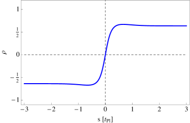
Similarly, like for the case of covariance, the correlation coefficient $\rho$ saturates for $s\rightarrow\pm\infty$. Therefore, one can infer that also a product of uncertainties $\Delta\hat{Q}\Delta\hat{P}$ approaches asymptotically some finite, nonzero values. Furthermore, it is worth mentioning that in contrast to $C_{QP}$, the correlation coefficient $\rho$ is not a monotonic function of $s$, so it cannot play the role of the intrinsic quantum parameter of time.

For a state with nonvanishing covariance, as the one studied here, the so-called Robertson-Schrödinger uncertainty relation holds Schrodinger:1930ty ,

$$(\Delta\hat{Q})^{2}(\Delta\hat{P})^{2}-C_{QP}^{2}\geq(\hslash/2)^{2},$$ (12)

which is a generalization of the Heisenberg uncertainty relation. The uncertainty relation is saturated, while the square of the left-hand side of the inequality (12) reaches the $\hslash/2$ value. Such a state of minimal uncertainty, usually corresponding to the vacuum state, is the least quantum state. In order to study how such state is approached within our model, we plot the square of the left-hand side of (12) as a function of time in Fig. 3.

Figure 3: Uncertainty $\sqrt{(\Delta\hat{Q})^{2}(\Delta\hat{P})^{2}-C_{QP}^{2}}$ for $\tilde{\alpha}=0.1$ and $\tilde{E}_{0}=10$. The shadowed region is prohibited in accordance with the uncertainty principle (12).

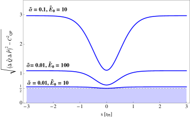
As we see, uncertainty reaches its minimum at the transition point between the contracting and expanding phases. Therefore, bounce can be viewed as the least quantum part of the evolution. The Universe can be best “localized” just at the bounce. In the next section, we will try to explain this counter-intuitive feature using entropy.

We have studied so far an evolution of covariance and dispersions for our model. Let us now combine this knowledge with evolution of mean values of the canonical variables and investigate evolution of the quantum system under consideration on the phase space. For this purpose, let us consider the covariance matrix,

$${\bf\Sigma}:=\left[\begin{array}[]{cc}(\Delta\hat{Q})^{2}&C_{QP}\\ C_{QP}&(\Delta\hat{P})^{2}\end{array}\right],$$ (13)

which is known in statistics. Since the ${\bf\Sigma}$ matrix is symmetric, it can be diagonalized ${\bf\Sigma}={\bf O}{\bf\Lambda}{\bf O}^{T}$, where ${\bf O}$ is the rotation matrix and the diagonalized matrix ${\bf\Lambda}=\text{diag}(\lambda_{+},\lambda_{-})$. The eigenvalues of matrix ${\bf\Lambda}$ can be expressed as follows:

$$\lambda_{\pm}=\frac{1}{2}\left[\text{tr}{\bf\Sigma}\pm\sqrt{(\text{tr}{\bf\Sigma})^{2}-4\det{\bf\Sigma}}\right],$$ (14)

where $\text{tr}{\bf\Sigma}=(\Delta\hat{Q})^{2}+(\Delta\hat{P})^{2}$ and $\det{\bf\Sigma}=(\Delta\hat{Q})^{2}(\Delta\hat{P})^{2}(1-\rho^{2})$. The square roots of $\lambda_{+}$ and $\lambda_{-}$ have interpretation of major and minor axes of the ellipsoid of covariance, respectively. An angle between the major axis and the $P$ axis (counting counterclockwise) is

$$\theta=\frac{1}{2}\arctan\left[\frac{2C_{QP}}{(\lambda\Delta\hat{Q})^{2}-(\Delta\hat{P}/\lambda)^{2}}\right].$$ (15)

It is worth noting that the angle $\theta$, in contrast to the covariance $C_{QP}$ and the coefficient $\rho$, is an explicit function of the parameter $\lambda$.

In Fig. 4 we show the parametric curve ($\langle\hat{Q}\rangle\lambda$, $\langle\hat{P}\rangle/\lambda$) for $\tilde{\alpha}=0.1$ and $\tilde{E}_{0}=10$ together with five exemplary ellipses of dispersion.

Figure 4: An open curve corresponds to the plot ($\langle\hat{Q}\rangle\lambda$,$\langle\hat{P}\rangle/\lambda$) for $\tilde{\alpha}=0.1$ and $\tilde{E}_{0}=10$. Ellipses describe dispersion of state at five stages of evolution.

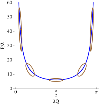
The dispersion of $\hat{Q}$ is largest at the bounce and tends to zero with the increase of $\langle\hat{P}\rangle$. In turn, the dispersion $\Delta\hat{P}$ reaches its minimum value at the bounce and grows with the increase of $\langle\hat{P}\rangle$. Furthermore, as can be inferred from the behavior of the ellipses of covariance, the state undergoes both amplitude and phase squeezing. This reflects the fact that both axes of the ellipse of covariance ($\sqrt{\lambda_{\pm}}$) as well as the phase factor $\theta$ are evolving in time.

IV Entropy

It is tempting to define the notion of entropy in quantum cosmology as it may be used in defining the cosmological arrow of time. The von Neumann definition of entropy for a quantum system reads $S=-k_{B}\text{tr}[\hat{\rho}\ln\hat{\rho}]$. Here, $k_{B}$ is the Boltzmann constant and $\hat{\rho}$ is the density matrix for a quantum state. The von Neumann entropy is defined in such a way that it vanishes for the pure states $|\Psi\rangle$, for which $\hat{\rho}=|\Psi\rangle\langle\Psi|$. One argues that since an evolution of the pure state is unitary, there is no information loss so the entropy remains unchanged. On the other hand, for mixed states, information about the quantum system can be lost due to the entanglement with environment and the von Neumann entropy is increasing. In particular, in quantum cosmology, degrees of freedom can be decomposed for relevant and irrelevant as already mentioned in the Introduction. The irrelevant degrees of freedom may play a role of the environment that causes decoherence of the sector parametrized by the relevant degrees of freedom as the scale factor. Making some qualitative analysis of the Wheeler-DeWitt equation one may show that the resulting von Neumann entropy is a monotonically increasing function of a scale factor for the FRW model Zeh ; Kiefer:2005vd . This is in agreement with expectations based on thermodynamical arguments for the expanding Universe. Moreover, such dependence indicates that quantum entropy should decrease in the contracting Universe. This may suggest, by applying the second law of thermodynamics, that the arrow of time is directed out of the bounce and only expansion has physical meaning Kiefer:2005vd .

In the case discussed above, the entropy production was due to the entanglement with the environment containing irrelevant degrees of freedom. However, while considering the minisuperspace model of quantum cosmology, as the one studied in this paper, one usually does not refer to the whole superspace and therefore no entropy growth is expected, as for the pure states. This is however not physically true and results from oversimplification of the system under consideration. However, we suppose that the information about an entropy can be extracted from the state of the minisuperspace model. This is because a form of this state is determined by the process of decoherence, which takes into account the environmental degrees of freedom. As already mentioned in the Introduction the resulting states are usually Gaussian packets, as the one considered here.

Based on the above information, we derive the conclusion that the other definition of entropy should be used in such a case, which may give nonvanishing entropy also for some pure states. In fact, such an idea is not a new one. Especially, the relation between the degree of squeezing of a quantum state and entropy was discussed Gasperini:1993mq . It was shown that in the case of quantum cosmological perturbations, the entropy of the squeezing pure semiclassical states and the von Neumann entropy may lead to the same results Gasperini:1995yd . An idea of relating quantum evolution for pure states with the arrow of time and entropy was also discussed by Bojowald et al. Bojowald:2008by ; Bojowald:2009kb .

We propose the following definition of entropy measuring the degree of squeezing of a quantum state:

$$S:=k_{B}\ln\left(\frac{\Delta\hat{Q}\Delta\hat{P}\sqrt{1-\rho^{2}}}{\hslash/2}\right).$$ (16)

This definition can be generalized to the cases with a higher number of degrees of freedom. Definition (16) may be viewed as a quantum analogue of the Boltzmann entropy $S=k_{B}\ln\Omega$, where $\Omega$ is the number of microstates in the microcanonical ensemble. The minimal volume of phase space, which can be occupied by the quantum system is obtained by saturating the Heisenberg (or Robertson-Schrödinger) relation so it is equal to $\Gamma_{0}=\hslash/2$. Therefore, $\Gamma/\Gamma_{0}$, where $\Gamma:=\Delta\hat{Q}\Delta\hat{P}\sqrt{1-\rho^{2}}=\sqrt{\lambda_{+}\lambda_{-}}$ ($\sim$ area of ellipse of covariance), is approximately the number of elementary cells $\Gamma_{0}$ covered by the ellipsoid of covariance. This number of cells is an analogue of the number of microstates $\Omega$ in a given macrostate.

One can also show that equation (16) can be derived from the Gibbs formula. Taking into account only first and second order quantum moments to describe our system, the Wigner function can be approximated by the Gaussian distribution

$$W(Q,P)=\frac{1}{2\pi\sqrt{\det{\bf\Sigma}}}\exp\left(-\frac{1}{2}{\bf x}^{T}{\bf\Sigma}^{-1}{\bf x}\right)$$ (17)

where ${\bf x}=(Q-\langle\hat{Q}\rangle,P-\langle\hat{P}\rangle)$. The Wigner function is strictly a positive function here, reflecting semiclassical nature of the state under considerations. Moreover, the Wigner function fulfills the normalization condition

$$\int_{-\infty}^{+\infty}dQ\int_{-\infty}^{+\infty}dP\ W(Q,P)=1.$$ (18)

For the sake of simplicity, we have extended here ranges of $Q$ and $P$ variables to $\mathbb{R}$. This approximation is however well satisfied for the considered Gaussian state. Namely, by looking at Fig. 4, we see that the ellipses of dispersions are placed well within the region $[0,\pi]\times\mathbb{R}_{+}$. Therefore, contributions from the region outside of $[0,\pi]\times\mathbb{R}_{+}$ to the Wigner function (17) is marginal.

Using the Wigner function (17) as a phase space density distribution in definition of the Gibbs entropy we obtain

$$S = -k_{B}\int_{-\infty}^{+\infty}dQ\int_{-\infty}^{+\infty}dP\ W(Q,P)\ln(W(Q,P))$$ (19)

$$= k_{B}(1+\ln\pi)+k_{B}\ln\left(\frac{\sqrt{\det{\bf\Sigma}}}{\hslash/2}\right)$$

$$= k_{B}(1+\ln\pi)+k_{B}\ln\left(\frac{\Delta\hat{Q}\Delta\hat{P}\sqrt{1-\rho^{2}}}{\hslash/2}\right),$$

where we restored the Planck constant $\hslash$. So, the Gibbs entropy leads to formula (16) up to the constant factor $k_{B}(1+\ln\pi)$. It is worth stressing that it was possible to use here the Wigner function, only because it was positive for the state under consideration. However, in case of not strictly positive Wigner functions, one can still construct the corresponding Husimi $Q$ function being positively defined. In this case, the above Gibbs formula applied to the Husimi distribution leads to so-called Wehrl entropy Wehrl:1978zz .

In Fig. 5, we present an evolution of the entropy (16) for our system.

Figure 5: Entropy in the bouncing cosmology.

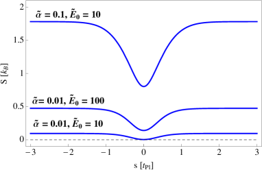
The entropy reaches the minimum value at the bounce while saturated for $s\rightarrow\pm\infty$. This behavior is qualitatively similar to what was predicted by the von Neumann entropy with environmental degrees of freedom taken into account Zeh ; Kiefer:2005vd .

Making use of the above reasoning, we can give an interpretation to the fact that for the Gaussian state the total uncertainty $\Delta\hat{Q}\Delta\hat{P}\sqrt{1-\rho^{2}}$ has a minimum at the bounce: quantum entropy grows with the increase of volume. Furthermore, if the second law of thermodynamics applies to the entropy defined by equation (16), one could expect that entropic arrows of time are directed out of the point of bounce. In such a case, only the expansion of the Universe can be perceived by the internal observer. Such an interpretation differs from the standard understanding of the phase of bounce as successive contraction and expansion. This standard point of view is additionally supported by the presence of internal quantum time played by covariance, as shown in the previous section.

V Relative fluctuations

The relative fluctuation of an observable $\mathcal{O}$, defined as $\delta(\mathcal{O}):=\Delta\hat{\mathcal{O}}/{\langle\hat{\mathcal{O}}}\rangle$ (where ${\langle\hat{\mathcal{O}}}\rangle$ is the expectation value of $\mathcal{O}$), is a sort of a gauge for measuring the cosmic amnesia. The relative fluctuations $\delta(P)$ are symmetric with respect to the bounce, as shown in Fig. 6.

Figure 6: Relative fluctuations of $\hat{P}$.

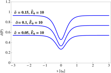
They saturate on $\delta(P)|_{\text{max}}$ while $s\rightarrow\pm\infty$ and reach the minimum at the bounce. Therefore, if the semiclassicality condition $\delta(P)\ll 1$ is imposed in the expanding phase, it constrains the rest of the evolution.

In the case of the $\hat{Q}$ observable, the relative fluctuations $\delta(Q)$, presented in Fig. 7,

Figure 7: Relative fluctuations of $\hat{Q}$.

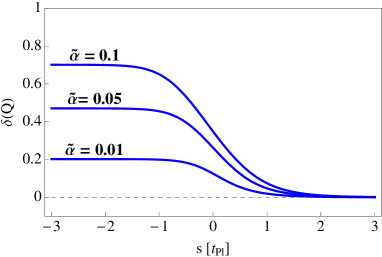
are asymmetric with respect to the bounce and only become symmetric when $\tilde{\alpha}\rightarrow 0$. For $s\rightarrow-\infty$, the $\delta(Q)$ saturates at $\delta(Q)|_{\text{max}}=\sqrt{e^{4\tilde{\alpha}}-1}$, while it tends to zero for $s\rightarrow+\infty$. Since the directions of the evolution parameter $s$ and cosmological time $t$ are opposite, the relative fluctuations $\delta(Q)$ monotonically grow in the cosmological time.

From the point of view of the possible observability (detection) of the amnesia, the observable $\hat{Q}$ is a favorite because in the classical limit, $Q=\gamma H$, where $H$ is the Hubble parameter and $\gamma$ is Barbero-Immirzi parameter. Therefore, relative fluctuations of $\hat{Q}$ can be constrained observationally. In contrast, it is hard to put any constraint on $\delta(P)$, because $P$ is linked to the physical volume of space $v=4\pi G\gamma P$, which is not measurable.

The relative fluctuations $\delta(Q)$ at the given time cannot be greater than the relative uncertainty of measurement. In particular, the present value of the Hubble factor is $H_{0}=70.2\pm 1.4\ \text{km}\ \text{s}^{-1}\ \text{Mpc}^{-1}$ Komatsu:2010fb , thus we have the constraint $\delta(Q)<\frac{\sigma(H_{0})}{H_{0}}\approx 0.02$. Another constraint can be derived for the phase of inflation, based on observations of the cosmic microwave background (CMB) radiation. If the inflation was driven by a massive inflaton field, the Hubble factor $H_{*}=\frac{1}{2}m_{\text{Pl}}\sqrt{\mathcal{A}_{s}\pi(1-n_{s})}$, where $\mathcal{A}_{s}$ is the amplitude of scalar perturbations and $n_{s}$ is the corresponding spectral index. From the seven years of observations of the WMAP satellite combined with other cosmological measurements $\mathcal{A}_{s}=(2.430\pm 0.091)\cdot 10^{-9}$ and $n_{s}=0.968\pm 0.012$ Komatsu:2010fb . Based on this we find the constraint $\delta(Q)<\frac{\sigma(H_{*})}{H_{*}}\approx 0.19$. The future measurements of the B-type polarization of the CMB will allow to determine $H_{*}$ with higher precision and therefore improve the above constraint.

The model we consider applies to the vicinity of Planck’s epoch, however if assuming that the quantum fluctuations are not decreasing thereafter, the derived observational bound can be used to constraint $\delta(Q)|_{\text{max}}$. From the first constraint $\delta(Q)|_{\text{max}}<0.02$, which translates into $\tilde{\alpha}<10^{-4}$ and from the second one $\delta(Q)|_{\text{max}}<0.19$, leading to $\tilde{\alpha}<9\cdot 10^{-3}$. Both constraints suggest that the semiclassicality condition was indeed fulfilled. Therefore, because constraint $\delta(Q)|_{\text{max}}<1$ implies $\delta(P)|_{\text{max}}<1$, one can conclude that there is no cosmic amnesia within the considered model.

VI Summary and conclusions

In this paper, we have studied quantum dynamics, using the Gaussian state, of the FRW cosmological model with a free scalar field in the framework of the reduced phase space loop quantum cosmology.

We have analyzed evolution of the first and second order moments of the canonical variables. By investigating quantum uncertainties, we have shown that the phase of the bounce is the least quantum part of the evolution. We have also shown that covariance is a monotonic function of the time parameter. Therefore, it may serve as an intrinsic quantum parameter of time.

We have introduced the notion of the entropy of squeezing and analyzed its behavior for the the quantum state under considerations. We have shown that the resulting scale factor dependence of entropy is in qualitative agreement with the results based on the von Neumenn entropy for the mixed states.

We have shown that the $\hat{Q}$ observable, not the $\hat{P}$ observable, should be used as a tool for studying (within the FRW model) the reality of the cosmic forgetfulness. It is so because only relative fluctuations of $\hat{Q}$ can be constrained observationally, contrary to the fluctuations of $\hat{P}$. The available cosmological data allow one to constrain the relative fluctuations $\delta(Q)$. Using these data, we have shown that the semiclassicality is preserved across the bounce.

Since the dependance of $\Delta\hat{Q}\Delta\hat{P}\sqrt{1-\rho^{2}}$ on time is symmetric with respect to the bounce, our quantum universe is equally quantum before and after the bounce, in the context of uncertainty principle. In this sense, the Universe remembers its quantumness across the bounce.

In papers BojowaldNature ; Bojowald:2007gc , the authors consider a solvable toy model (motivated by the LQC) to argue that a quantum state before the bounce may become semiclassical after the bounce. The authors of Corichi:2007am ; Corichi:2011rt criticize these results claiming that the cosmic amnesia is only an artifact of poor analyzes of a simple toy model. In Corichi:2007am ; Corichi:2011rt , the authors examine the same cosmological model as we do, but within the sLQC method (simplified LQC). However, they mainly examine the $\hat{P}$ observable. Since $\delta(P)$ is symmetric with respect to the bounce, they obviously cannot see any indications of the cosmic amnesia. Also the sophisticated calculations presented in Kaminski:2010yz concern mainly $\delta(P)$.

Further analysis can be done by calculating an evolution of $\delta(Q)$ for the FRW model with a scalar field potential. This would enable obtaining more accurate constraints from the CMB observations.

We are conscious that our results may depend on the choice of the initial state. Therefore, we have been working on the extension of our investigation considering a variety of semiclassical states JKW . For such states, the mean values follow the classical trajectories as in the case of the Gaussian state. However, evolution of quantum fluctuations may differ from the case described here. In particular, one can construct a squeezed vacuum state for which dispersions of elementary variables remain constant during evolution, but the covariance is varying in time.

Our classical Hamiltonian is unique for a given choice of an evolution parameter (time). But, it is commonly known that quantization of an observable may suffer from ambiguities. In our next paper JKW , we consider different factor ordering of elementary variables defining the Hamiltonian to test the sensitivity of our results to this procedure.

The issues raised above require performing extensive calculations, which are beyond the scope of the present paper.

An extension of our results to the Bianchi type universes Dzierzak:2009dj ; Malkiewicz:2010py is another direction in our cosmology program. Some evidence indicating possible relevance of anisotropic effects is connected with an observed CMB anomaly called the “axis of evil” Land:2005ad . This is another motivation, apart from the BKL results, for applying the homogeneous models to describe the very early Universe.