Constraints on the Synchrotron Shock Model for the Fermi GBM Gamma-Ray Burst 090820A

Abstract

Discerning the radiative dissipation mechanism for prompt emission in Gamma-Ray Bursts (GRBs) requires detailed spectroscopic modeling that straddles the $\nu F_{\nu}$ peak in the 100 keV - 1 MeV range. Historically, empirical fits such as the popular Band function have been employed with considerable success in interpreting the observations. While extrapolations of the Band parameters can provide some physical insight into the emission mechanisms responsible for GRBs, these inferences do not provide a unique way of discerning between models. By fitting physical models directly this degeneracy can be broken, eliminating the need for empirical functions; our analysis here offers a first step in this direction. One of the oldest, and leading, theoretical ideas for the production of the prompt signal is the synchrotron shock model (SSM). Here we explore the applicability of this model to a bright Fermi GBM burst with a simple temporal structure, GRB 090820A. Our investigation implements, for the first time, thermal and non-thermal synchrotron emissivities in the RMFIT forward-folding spectral analysis software often used in GBM burst studies. We find that these synchrotron emissivities, together with a blackbody shape, provide at least as good a match with the data as the Band GRB spectral fitting function. This success is achieved in both time-integrated and time-resolved spectral fits.

1. Introduction

In the most popular paradigm for gamma-ray bursts of both long and short durations, it is typically assumed that prompt $\gamma$-ray emission results from the dissipation of kinetic energy in a relativistically expanding fireball mediated by multiple internal shocks (e.g. see Piran 1999, or Mészáros 2001, for reviews). These shocks are presumed to diffusively accelerate a fraction of the electrons from thermal upstream distributions to higher energies. Usually only particles in the exponential tail of the Maxwellian are available for acceleration. Thus, for relativistic shocks, the expected outcome is that the particle distribution consists of a Maxwellian with a power-law tail at high energies. Based on this scenario, the radiative emission should consist of two components, quasi-thermal and non-thermal photons from electrons spiralling along magnetic field lines in optically thin regions of the jet. There could also be an additional photospheric contribution of Planckian form, originating in distinct, optically thick environs, perhaps interior to the regions spawning synchrotron emission.

To date, the characterization of GRB spectra has been dominated by the use of the empirical Band function (Band et al., 1993), a parametrized, smoothly broken power law that was devised in the era of the BATSE experiment on the Compton Gamma-Ray Observatory (CGRO). Several authors have used measurements of the Band spectral shape parameters to infer properties of the physics involved in GRB emission. In particular, the fitted spectral indices defined by $N_{\gamma}\propto E^{-\alpha}$ below the $\,\nu F_{\nu}\,$ peak and $N_{\gamma}\propto E^{-\beta}$ above it, may be compared with values predicted from synchrotron emission: the low-energy self-absorption index, $\alpha$, of $+1$ (in photon flux units), the synchrotron ‘line of death’ index of $-2/3$, the ‘second line of death’ at the fast cooling value of $-3/2$, the high energy index, $\beta$, characterizing power-law particle acceleration, and the various spectral differences between these (Preece et al., 1998; Lloyd & Petrosian, 2000; Lloyd-Ronning & Petrosian, 2002; Preece et al., 2002). However, it becomes difficult to discern between models through the Band function when the fitted low energy indices represent a power law only asymptotically, and when many models predict similar Band indices. In fact, the Band function’s inherent shape and curvature only loosely approximates the shape of the applicable physical models making it difficult to draw conclusions about emission mechanisms directly from Band function fits. A way to break this degeneracy is by fitting more realistic emission models to the data, which in addition provides deeper insights into the burst environment. In Section 2 we detail the emission model that we use to fit GRB spectra. We present this model as a first step. In future work we will explore additional models in an attempt to discern between them. We describe our observational results with this model in Section 3.

2. Model and Motivation

We propose to test an emission model composed of synchrotron emission and a thermal blackbody. This model is the most general form of the standard fireball model. Non-thermal synchrotron emission is historically the most favored process invoked to explain prompt GRB signals. The motivation for the inclusion of a blackbody component comes not only from theory (Goodman, 1986; Mészáros, 2002; Rees & Mészáros, 2005) and previous searches (Ryde and Pe’er, 2009) but also the recent discovery of a significant quasi-thermal component in GRB spectra (Guiriec et al., 2010; Ryde et al., 2010). However, in Guiriec et al. (2010; GRB 100724B) as well as Ryde et al. (2010; GRB 090902B), the non-thermal portion of the spectra is approximated by empirical functions that lack direct associations with the physical parameters.

In order to model optically-thin synchrotron emission in a physical way, we adopt the parametrization presented in Baring & Braby (2004, hereafter BB04), which was modified slightly from the choice of Tavani (1996). Theory and numerical simulations predict that the electron energy distribution resulting from diffusive shock acceleration should be composed of two components (e.g. see Baring 2011 for an overview), which to first order can be approximated by a superposition of a relativistic Maxwellian and a super-thermal power-law tail:

$$n_{e}(\gamma)\;=\;n_{0}\biggl{[}\;\Bigl{(}\hbox{${{\displaystyle\gamma\vphantom{(}}\over{\displaystyle\gamma_{\hbox{\fiverm T}}\vphantom{(}}}$}\Bigr{)}^{2}\,e^{-\gamma/\gamma_{\hbox{\fiverm T}}}+\epsilon\,\Bigl{(}\hbox{${{\displaystyle\gamma\vphantom{(}}\over{\displaystyle\gamma_{\hbox{\fiverm T}}\vphantom{(}}}$}\Bigr{)}^{-\delta}\,\Theta\Bigl{(}\hbox{${{\displaystyle\gamma\vphantom{(}}\over{\displaystyle\eta\gamma_{\hbox{\fiverm T}}\vphantom{(}}}$}\Bigr{)}\,\biggr{]}\,,$$ (1)

where $\,\Theta(x)\,$ is a step function with $\,\Theta(x)=1\,$ for $\,x\geq 1\,$ and zero otherwise, and $\,\gamma_{\hbox{\fiverm T}}\,$ is a measure of the post-shock electron temperature. This is a quasi-isotropic distribution, in the comoving frame of reference of the GRB outflow (the mildly-relativistic speed of an internal shock in this frame does not change this form significantly), with the dependence on pitch angle being omitted for simplicity, though it can be incorporated in the $\,n_{0}\,$ factor. The shock acceleration electron distribution therefore depends on five parameters, three of which, the power-law index, $\,\delta\,$, the relative normalization, $\,\epsilon\,$ (which can be related to the acceleration efficiency), and the product $\,\eta\gamma_{\hbox{\fiverm T}}\,$, which defines the minimum Lorentz factor of the power-law, pass unmodified into the expression of the photon flux and are thus fit parameters for the GRB data. In Tavani’s original exposition $\,\eta\,$ was fixed to unity and the power law component smoothly joined to the exponential portion of the Maxwellian (i.e., with virtually no discontinuity). This would be the case of ‘saturated’ acceleration, where all of the electrons above the peak in the Maxwellian have been accelerated. BB04 indicated that values $\,\eta\sim 3\,$ and $\,\epsilon\mathrel{\mathchoice{\lower 2.0pt\vbox{\halign{$\m@th\displaystyle\hfil#\hfil$\cr<\crcr\sim\crcr}}}{\lower 2.0pt\vbox{\halign{$\m@th\textstyle\hfil#\hfil$\cr<\crcr\sim\crcr}}}{\lower 2.0pt\vbox{\halign{$\m@th\scriptstyle\hfil#\hfil$\cr<\crcr\sim\crcr}}}{\lower 2.0pt\vbox{\halign{$\m@th\scriptscriptstyle\hfil#\hfil$\cr<\crcr\sim\crcr}}}}0.1\,$ closely reflect populations usually found in simulations of shock acceleration even ones based on diverse and contrasting approaches (e.g. see Niemiec & Ostrowski 2004; Spitkovsky 2008; Baring 2011; and references therein). For simplicity and general facility of spectral fitting, we adopt the compact form in Eq. (1), deferring direct fitting with specific simulation model output to future studies. Here, $\,\eta=3\,$ is adopted as a representative value that incurs no significant discontinuity in transitioning from the Maxwellian to the non-thermal population when $\,\epsilon\mathrel{\mathchoice{\lower 2.0pt\vbox{\halign{$\m@th\displaystyle\hfil#\hfil$\cr<\crcr\sim\crcr}}}{\lower 2.0pt\vbox{\halign{$\m@th\textstyle\hfil#\hfil$\cr<\crcr\sim\crcr}}}{\lower 2.0pt\vbox{\halign{$\m@th\scriptstyle\hfil#\hfil$\cr<\crcr\sim\crcr}}}{\lower 2.0pt\vbox{\halign{$\m@th\scriptscriptstyle\hfil#\hfil$\cr<\crcr\sim\crcr}}}}0.1\,$.

In a truly physical model, the electron distribution function should be perfectly continuous, contrasting Eq. (1). Here, we have left both $\,\eta\,$ and $\,\epsilon\,$ as parameters free to vary, observing that folding the distribution with the synchrotron emissivity function in Eq. (2) below yields continuous emission spectra. Thus, while not explicitly joining the two components of Eq. (1) smoothly, the subsequent fitting of GRB spectral data provides a robust and informative indication concerning the relative contribution of each component, as was done in BB04. More precise modeling with truly continuous electron distributions is left for future investigations, but is unlikely to alter the essential conclusions of our work here.

To determine the radiation flux, $\,F_{\nu}(\mathcal{E})\propto\mathcal{E}N_{\gamma}\,$, emitted by these electrons, this distribution is convolved with the standard synchrotron emissivity (e.g. Rybicki and Lightman, 1979; see also BB04):

$$F_{\nu}(\mathcal{E})\;\propto\;\int_{1}^{\infty}n_{e}(\gamma)\,\mathcal{F}\left(\hbox{${{\displaystyle\mathcal{E}\vphantom{(}}\over{\displaystyle\mathcal{E}_{c}\vphantom{(}}}$}\right)\,d\gamma\quad,$$ (2)

where

$$\mathcal{F}\left(w\right)\;=\;w\int_{w}^{\infty}K_{5/3}(x)\,dx$$ (3)

expresses the single-particle synchrotron emissivity (i.e. energy per unit time per unit volume) in dimensionless functional form. The characteristic scale for the synchrotron photon energy is

$$\mathcal{E}_{c}\;=\;\hbox{${{\displaystyle 3\vphantom{(}}\over{\displaystyle 2\vphantom{(}}}$}\;\hbox{${{\displaystyle B\vphantom{(}}\over{\displaystyle B_{\rm cr}\vphantom{(}}}$}\,\Gamma\,\gamma^{2}\,m_{e}c^{2}\quad,$$ (4)

where $\,B_{\rm cr}=4.41\times 10^{13}\,$Gauss is the quantum critical field. When convolved with the distribution in Eq. (1), the substitution $\,\gamma\to\eta\gamma_{\hbox{\fiverm T}}\,$ in Eq. (4) then defines the scale for the break energy of the synchrotron continuum resulting from the truncated power-law portion of the distribution (see Table 1). In modeling prompt burst emission, the relativistic nature of the outflow introduces an extra parameter, the bulk Lorentz factor $\,\Gamma\,$ of the flow, which blueshifts the spectrum so as to introduce the $\,\Gamma\,$ factor in Eq. (4), so that Eq. (2) then expresses the synchrotron flux in the observer’s frame. Accordingly, while the electron distribution parameters $\,\delta\,$ and $\,\epsilon\,$ can be constrained by prompt emission spectroscopy, the precise values of $\,\gamma_{\hbox{\fiverm T}}\,$ and the environmental quantities $\,B\,$ and $\,\Gamma\,$ are indeterminate, being subsumed in the single parameter $\,\Gamma\eta^{2}\gamma_{\hbox{\fiverm T}}^{2}B\,$ that is defined by a spectral fit in a given time interval.

For fits where non-thermal synchrotron components dominate, the energy of the $\,\nu F_{\nu}\,$ peak determines the value of the peak energy. Well below this structure the flux index is $\,+1/3\,$ and well above it, the flux index is $\,-(\delta-1)/2\,$. This is the simplest synchrotron model to consider. Strong cooling synchrotron models possess a similar mathematical character, but elicit a gentler break and a steeper spectrum below the break that is often more difficult to fit to observations. Treatment of such cooling models, and inverse Compton scenarios will be deferred to future work. We note also that models where $\,\epsilon\ll 1\,$ and the non-thermal synchrotron component is small or insignificant, the high energy tail of the thermal synchrotron component is necessarily exponentially declining with energy. Such forms have severe difficulty in fitting GRB spectra that possess extended power-law tails, a common occurrence, yielding $\,\epsilon\mathrel{\mathchoice{\lower 2.0pt\vbox{\halign{$\m@th\displaystyle\hfil#\hfil$\cr>\crcr\sim\crcr}}}{\lower 2.0pt\vbox{\halign{$\m@th\textstyle\hfil#\hfil$\cr>\crcr\sim\crcr}}}{\lower 2.0pt\vbox{\halign{$\m@th\scriptstyle\hfil#\hfil$\cr>\crcr\sim\crcr}}}{\lower 2.0pt\vbox{\halign{$\m@th\scriptscriptstyle\hfil#\hfil$\cr>\crcr\sim\crcr}}}}0.1\,$ as an anticipated frequent inference in this GRB spectroscopy protocol.

In summation, our emission model consists of a two-component synchrotron function (thermal and power-law), plus a blackbody, all boosted from the outflow frame, by the bulk Lorentz factor $\,\Gamma\,$, to the observer’s frame. Along with the blackbody component, this spectral model has seven fit parameters; values for two of these parameters, $\,\eta\,$ and $\,\delta\,$, are fixed for reasons detailed in Section  3. Owing to the intensive numerical integration involved, such functions have previously not been used for forward-folding spectral fitting, particularly in the CGRO/BATSE era. We have implemented this photon model into the RMFIT spectral analysis software and demonstrate our technique by fitting fitting the prompt emission of GRB 090820A; one of the brightest GBM bursts with simple temporal structure.

3. Observations

On 20 August 2009, at T₀=00:38:16.19 UT, the Gamma-Ray Burst Monitor (GBM) onboard the Fermi Gamma-ray Space Telescope triggered on the very bright GRB 090820A (Connaughton, 2009). This GRB also triggered Coronas Photon-RT-2 (Chakrabarti et al., 2009). The burst location was initially not in the FOV of the Large Area Telescope (LAT) onboard Fermi but was bright enough to result in a Fermi spacecraft repointing maneuver. However, Earth avoidance constraints prevented such a maneuver until 3100 sec after the burst trigger and the burst was not detected at higher energies by the LAT. The most precise position for the direction of the burst comes from the GBM trigger data which localizes the burst to a patch of sky centered on RA = 87.7 degree and Dec = 27.0 degree (J2000) with a 4 degree error, statistical and systematic. The current best model for systematic errors is 2.8 degrees with 70% weight and 8.4 degrees with 30% weight (Briggs et al., 2011). We verified that our analysis does not change significantly using instrument response functions for assumed source locations throughout this region of uncertainty.

GBM is composed of 12 sodium iodide (NaI) detectors covering an energy range from 8 keV to 1 MeV and two bismuth germanate (BGO) detectors sensitive between 200 keV and 40 MeV (Meegan et al., 2009). Figure 1 (top two panels) shows the light curve of GRB 090820A as seen by GBM, from 8 to 200 keV in the NaI detectors (top) and from 200 keV to 40 MeV in the BGO detector (bottom). GBM triggered on a weak precursor which we do not include in the analysis. The main light curve begins at T₀ + 28.1s. The main structure of the light curve consists of a fast rising pulse with an exponential decay lasting until T₀+60 s. A second, less intense, peak beginning at T₀+30 s is superimposed on the main peak. With such a high intensity and simple structure, this GRB allows for detailed time-resolved spectroscopy. Because this burst is intense, calibration issues make the Iodine K-edge (33 keV) prominent in the count spectra owing to small statistical uncertainties, and we remove energy channels contributing to this feature from our spectral fits. In addition, an effective area correction is applied between each of the NaI detectors and the BGO 0 during the fit process. This correction of $\approx$ 23% is used to account for possible imperfections in the response models of the two detector types.

We simultaneously fit the spectral data of the NaI detectors with a source angle less than 60 degrees (NaI 1 and 5) and the data from the brightest BGO detector (BGO 0) using the analysis package RMFIT. We use a forward-folding technique that convolves the detectors’ response with the proposed photon model to generate a count spectrum to compare to the data; the parameters of the photon model are then adjusted so as to optimize the Castor C-stat statistic. The Castor C-stat differs from Poisson likelihood by an offset which is a constant for a particular dataset.

We perform a fit to the integrated spectrum and find that it is best represented by synchrotron emission from thermal and power-law distributed electrons with an additional blackbody component characterized by a kT $\approx$ 42 keV (C-Stat/DOF = 558/353). The $\,\nu F_{\nu}\,$ spectrum is displayed in Figure 2 and the best-fit values in Table 1. We also performed a fit using the Band function (C-Stat/DOF = 593/355). We find in concordance with BB04 that emission from power-law synchrotron dwarfs the emission from thermal synchrotron by at least 3 orders of magnitude. The value of $\eta$ is fixed to 3, the choice adopted by BB04: it is a value that accommodates distributions typically determined by shock acceleration simulations. When fitting the power-law synchrotron component we have to fix the value of the power-law index to its best fit value to remove a correlation between the amplitude and the index; this does not change the fit statistic but does mean that the amplitudes obtained are valid only for that index. The inferred electron distribution from this fit is shown in Figure 3. We note that the inability to simultaneously constrain the power-law index and amplitude of the synchrotron function may be solved in future studies by including joint fits with LAT data, whenever available.

For the time resolved analysis we fit four bins labeled a, b, c and d as shown in Figure 1 with the various synchrotron models. The corresponding electron distributions inferred from these fits are displayed in Figure 5. We also fit the Band function to each spectrum to show that in nearly all cases the physical models can fit the data as well as the Band function. We chose the time binning by finding a balance between high signal-to-noise and evolution of the spectral shape so that we can identify the time evolution of each component throughout the burst. Where possible, we fit all three components simultaneously. Due to the similarity in the spectral shapes of the low energy portions of the thermal synchrotron and power-law synchrotron components it is not always possible to constrain all of the fit parameters especially when one component is much stronger than the other. Therefore, when one component is dominant we include only that component in the fit. The ability to fit both components in the time integrated fit is most likely due to the fact that both components are significant over the interval.

From bins b to c the spectrum is best described by synchrotron emission from power-law distributed electrons in addition to a blackbody (Table 1 and Figure 4). The thermal synchrotron component is too weak to meaningfully include it in the fit. We find that the intensity of the power-law synchrotron increases significantly from bin b to c while the blackbody component remains nearly constant in intensity. The spectral index of the electrons in these intervals varies from -4.4 to -5.9. Such values are consistent with those expected from diffusive acceleration theory, for the specific case of superluminal shocks (Baring, 2011), i.e. those where the mean magnetic field angle to the shock normal is significant. This geometrical requirement establishes efficient convection of particles downstream of relativistic shocks, thereby steepening their acceleration distribution. The blackbody component decreases in intensity at this point but the temperature remains constant within errors. In bins a and d, with weaker emission, several models are essentially statistically tied. It is possible that PLS+BB persists throughout the entire GRB. Alternatively, the GRB could even begin in bin a with thermal synchrotron emission and transition to the PLS+BB emission. If this were true we would be seeing emission from electrons that have not yet been accelerated into a power-law distribution by the shock. The C-stat values for all of the models fit in each bin are displayed in Table 2.

While it is not possible to constrain all parameters in all the bins, it should be stressed that this is due to natural correlations in the synchrotron functions. These difficulties do not arise when using the Band function because it has a simpler parametrization.

4. Discussion and Conclusions

In this paper, we have shown that thermal and non-thermal synchrotron photon models, with an additional blackbody, are well consistent with the emission spectra of GRB 090820A in various time intervals. These are physical models that afford the ability to constrain parameters that are physically meaningful, for example key descriptors of the electron distribution that is motivated by shock acceleration theory. By implementing these models into a forward-folding spectral analysis software we have been able to directly constrain many of the physical model parameters and their respective errors; a first in the field of GRB spectroscopy. This constitutes substantial progress over the use of the empirical Band function to fit prompt GRB spectra, which has been a nearly universal practice to date. The results presented here enable more rigorous statements about the validity of GRB emission models, moving the study of prompt burst emission into a new era.

Our modeling has focused on the standard synchrotron shock model with the addition of a blackbody component. The spectral fitting reveals a complex temporal evolution of the separate components. While spectral evolution is a well-known feature of GRBs, this type of fitting can enable direct physical interpretation of the evolution. These fits provide evidence that the line of death issue (Preece et al. 1998, 2002) can be overcome naturally with a combination of synchrotron and blackbody emission: the prominence of a blackbody component with its flat Rayleigh-Jeans portion would derive a comparably-fitted Band function with a flat low-energy index. This was also suggested by Guiriec et al. (2010) where the authors used simultaneous fits of the Band function and a blackbody. Note that it is possible that other physical models may, in fact, produce superior fits to the data for GRB 090820A and other bursts. Strongly-cooled synchrotron emission, inverse Compton and jitter radiation are popular candidates, and our work here motivates the future development of RMFIT software modules for these processes.

A principal finding of the analysis in this paper is that the power-law synchrotron component is orders of magnitude more intense than the thermal synchrotron component during the peak of the burst, the latter contributing at most a few percent of the flux. This confirms the finding of BB04 for BATSE/EGRET bursts GRB 910503, GRB 910601 and GRB 910814, which was a theoretically-based perspective that did not fold models through the detector response matrices. They had noted that full plasma and Monte Carlo diffusion simulations of shock acceleration clearly predict a power-law tail in the particle distribution that smoothly extends from the dominant thermal population (e.g. see also Baring 2011, and references therein). This tail is several orders of magnitude smaller than what is found when fitting synchrotron emission to burst spectra. It is not clear how such non-thermally-dominated distributions can arise near shocks, providing a conundrum for the standard synchrotron shock model. Limited smoothing of the sharp peak of the non-thermal electron component will not alter this conclusion.

This result is also in accord with Guiriec et al. (2010), in their analysis of GRB 100724B, who fitted its GBM spectra with a combination of the Band model and a blackbody. They too found that an unrealistically high efficiency for the acceleration mechanism or a source size smaller than the innermost stable orbit of a black hole was required to invoke the standard fireball model for explaining the origin of the $\gamma$-ray emission. Therefore, it was surmised therein that the outflow from the jet was at least partially magnetized.

To conclude, the success of this analysis in isolating the relative contributions of a handful of distinct spectral components indicates that it is imperative for the field of GRB spectroscopy to move away from the use of the empirical fitting functions: many physical models can asymptotically approximate the Band spectral indices, rendering it difficult to discern between them particularly near the $\nu F_{\nu}$ peak. Instead, direct comparisons of the fitted physical models are possible, and are required to truly discriminate between the various emission processes. The fitting of physical SSM/blackbody spectra here offers a clear advance beyond empirical fits, and provides the impetus for further development and deployment of physical modeling of prompt burst emission spectra.

Figure 1.— Light curve of GRB 090820A as observed by GBM. The two panels show the count rate in the two NAI detectors (top) and BGO (bottom). The dashed lines indicate the time intervals (a, b, c, d) used for the time-resolved analysis (see Figure 3 and Table 1). It is clear that the burst consists of two main peaks and that this burst is very bright in the BGO detectors.

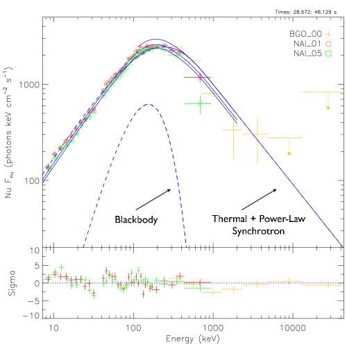
Figure 2.— The integrated spectrum of GRB 090820A. We are able to resolve three components, thermal synchrotron, power-law synchrotron, and a blackbody. Energy channels near the NaI K-edge are omitted. The deviations in the fit residuals are the due to systematics in the detector response resulting from the high count rate and spectral hardness of this burst. However, deviations are never greater than 4$\sigma$ and do not significantly impact the values of the best fit parameters. The multiple curves near the peak of the spectrum are an artifact of the effective-area correction applied to each detector and not related to the different fitted models.

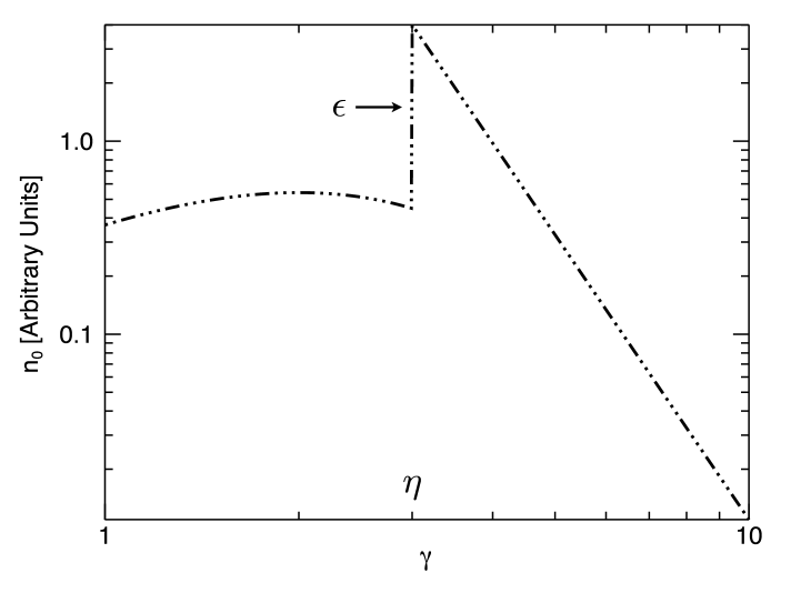
Figure 3.— The electron distribution corresponding to the integrated spectrum. The non-physical jump in the amplitude between the Maxwellian and the power-law distribution (parametrized by $\epsilon$) at $\eta$ is clearly seen.

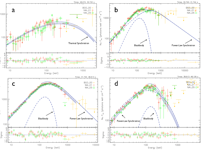
Figure 4.— The time-resolved spectra for GRB 090820A. The spectra represent bin a with thermal synchrotron only (top left panel), bin b with power-law synchrotron + blackbody (top right panel), bin c again with power-law synchrotron + blackbody (bottom left panel), and finally bin d with thermal synchrotron + blackbody (bottom right panel). As with Fig. 2, the multiple curves are associated with the effective area correction.

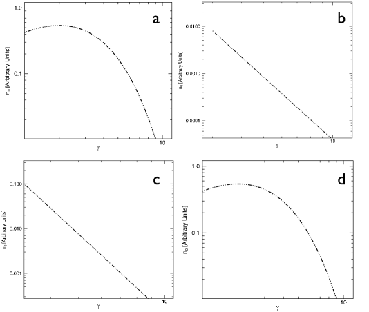
Figure 5.— The electron distributions for the time-resolved spectra. The choice of $\eta$ with a power-law only distribution is arbitrary due to the fact that $\mathcal{E}_{c}$ and $\eta$ both scale $E_{peak}$.

Table 1The fit parameters for the time-integrated (first row) and time-resolved spectra. The fit parameters for the blackbody component are its amplitude ($A_{BB}$) and energy ($kT$). The fit parameters for the non-thermal components are described in section 2. The break energy $\mathcal{E}_{b}\equiv\mathcal{E}_{c}(\gamma\to\eta\gamma_{\hbox{\fiverm T}})$ corresponds to employing the substitution $\gamma\to\eta\gamma_{\hbox{\fiverm T}}$ in Eq. (4). Note that the ratio of the amplitudes is not equal to the ratio of the fluxes.

Time interval	Model	$n_{0}$ $(\gamma s^{-1}cm^{-2}keV^{-1})$	$\epsilon$	$\mathcal{E}_{c}$ (keV)	$\delta$	$\eta$	$A_{BB}$ $(\gamma s^{-1}cm^{-2}keV^{-1})$	$kT$ (keV)
Time integrated	TS+PLS+BB	$0.3437_{-0.065}^{+0.204}$	$871_{-234}^{+254}$	$10.39_{-0.245}^{+0.254}$	$4.9\tablenotemark{a}$	$3.0$	$2.08_{-0.208}^{+0.367}\times 10^{-5}$	$42.27_{-1.35}^{+1.49}$
a	TS	$2.378_{-0.176}^{+0.189}$	$-$	$8.351_{-0.93}^{+1.08}$	$-$	$-$	$-$	$-$
b	PLS+BB	$859_{-89.1}^{+94.0}$	$-$	$14.24_{-0.776}^{+0.848}$	$4.4\tablenotemark{a}$	$3.0$	$1.774_{-0.356}^{+0.410}\times 10^{-4}$	$35.32_{-1.77}^{+1.99}$
c	PLS+BB	$1.901_{-0.093}^{+0.094}\times 10^{4}$	$-$	$15.22_{-0.399}^{+0.411}$	$5.9\tablenotemark{a}$	$3.0$	$1.818_{-0.344}^{+0.400}\times 10^{-4}$	$38.7_{-1.92}^{+2.13}$
d	TS+BB	$2.196_{-0.466}^{+0.720}$	$-$	$4.035_{-0.715}^{+0.689}$	$-$	$-$	$8.383_{-3.18}^{+4.89}\times 10^{-5}$	$28.40_{-3.59}^{+3.73}$

Time Interval	Band	TS	TS + BB	PLS	PLS + BB
a	464/355	466/357	464/355	467/357	465/355
b	432/355	742/357	445/355	555/357	434/355
c	450/355	1088/357	488/355	558/357	434/355
d	404/355	421/357	403/355	406/357	405/355

Table 2The c-stat per degree of freedom for each time model in the selected time intervals.

References

- Band et al. (1993) Band, D., Matteson, J., Ford, L., & Schaefer, B. 1993,ApJ, 413, 281.
- Baring (2011) Baring, M. G. 2011, Adv. Space. Res., 47, 1427.
- Baring & Braby (2004) Baring, M. G. & Braby, M. 2004, ApJ, 613, 460.
- Briggs et al. (2011) Briggs, M. S. et al. 2011 in preparation
- Connaughton (2009) Connaughton, V. 2009, GCN Circular 9829
- Chakrabarti et al. (2009) Chakrabarti, S., et al. 2009, GCN Circular 9833
- Goodman (1986) Goodman, J. 1986, ApJ, 308, L47.
- Guiriec et al. (2010) Guiriec, S., Connaughton, V., Briggs, M., & Burgess, M., et al. 2010, ApJ, 727, L33.
- Lloyd & Petrosian (2000) Lloyd, N. & Petrosian, V. 2000, ApJ, 543, 722.
- Lloyd-Ronning & Petrosian (2002) Lloyd-Ronning, N. & Petrosian, V. 2002, ApJ, 565, 182.
- Meegan et al. (2009) Meegan, C., et al. 2009, ApJ, 702, 791.
- Mészáros (2001) Mészáros, P. 2001, Science, 291, 79
- Mészáros (2002) Mészáros, P. 2002, AR & A, 40, 137.
- Niemiec (2004) Niemiec, J., & Ostrowski, M. 2004, ApJ, 610, 851.
- Piran (1999) Piran, T. 1999, Phys. Rep. 314, 575.
- Preece et al. (2002) Preece, R., Briggs, M. S., Giblin, T., & Mallozzi, R. 2002, ApJ, 581, 1248.
- Preece et al. (1998) Preece, R., et al. & Pendleton, G. N. 1998, ApJ, 506, L23.
- Rees & Mészáros (2005) Rees, M.J. and Mészáros, P. 2005, ApJ, 506, L23.
- Rybicki & Lightman (1979) Rybicki, G. & Lightman, A. 1979, Radiative Processes in Astrophysics (New York, Wiley and Sons)
- Ryde and Pe’er (2009) Ryde, F. and Pe’er, A. 2009, ApJ, 702, 1211.
- Ryde et al. (2010) Ryde, F., et al. , A. P. 2010, ApJ, 709, L172.
- Spitkovsky (2008) Spitkovsky, A. 2008, ApJ, 682, L5.
- Tavani (1996) Tavani, M. 1996, Phys. Rev. Lett. 76, 3478.