Scaling behavior of a square-lattice Ising model with competing interactions in a uniform field

Abstract

Transfer-matrix methods, with the help of finite-size scaling and conformal invariance concepts, are used to investigate the critical behavior of two-dimensional square-lattice Ising spin-$1/2$ systems with first- and second-neighbor interactions, both antiferromagnetic, in a uniform external field. On the critical curve separating collinearly-ordered and paramagnetic phases, our estimates of the conformal anomaly $c$ are very close to unity, indicating the presence of continuously-varying exponents. This is confirmed by direct calculations, which also lend support to a weak-universality picture; however, small but consistent deviations from the Ising-like values $\eta=1/4$, $\gamma/\nu=7/4$, $\beta/\nu=1/8$ are found. For higher fields, on the line separating row-shifted $(2\times 2)$ and disordered phases, we find values of the exponent $\eta$ very close to zero.

I Introduction

The study of frustration in magnetism has been a very active field of research in the recent past, both theoretically and experimentally. While experimentally-realizable frustrated magnets typically have a closer correspondence to quantum (i.e., Heisenberg or $XY$) spin models than to classical, Ising-like ones, their behavior turns out to be rather intricate. Thus, theoretical and/or numerical investigation of frustrated classical spin systems may, by virtue of their simplified character, help unravel some basic features which are common to frustrated magnets in general.

In this paper we investigate two-dimensional spin-$1/2$ Ising systems on a square lattice with first- and second-neighbor couplings, both antiferromagnetic, in the presence of a uniform magnetic field. The Hamiltonian is given by:

$${\cal H}=J_{1}\sum_{\rm NN}\sigma_{i}\,\sigma_{j}+J_{2}\sum_{\rm NNN}\sigma_{i}\,\sigma_{j}-H\sum_{i}\sigma_{i}\ ,$$ (1)

where $J_{1}$, $J_{2}>0$, NN and NNN stand respectively for next-neighbor and next-nearest-neighbor pairs, and $\sigma_{i}=\pm 1$. Here, all fields, coupling strengths and temperatures are given in units of $J_{1}$, unless otherwise stated. We have kept $J_{2}=1$ in all calculations reported in this work, except at the end of Sec. III.1, where $J_{2}=2$ and $0.75$ were briefly considered (both for $H=0$).

In line with the initial considerations given above, this may be considered a classical approximation for the $J_{1}-J_{2}$ (Heisenberg) model fm1 ; fm2 . Nevertheless, as shown in the following, the model described by Eq. (1) exhibits intricate features of its own, several of which are not fully understood so far. Depending on the relative strength of the associated parameters, such setup of competing interactions can generate various types of ordered phases at low temperature; more often than not, the transitions between these and the high-temperature (paramagnetic) state do not belong to the standard Ising universality class yl09 ; kalz08 .

The problem studied here has been analyzed by several numerical techniques in the past; Refs. yl09, ; kalz08, provide excellent summaries of earlier work, as well as illustrations of the use of up-to-date Monte-Carlo (MC) simulation techniques for this case.

We use transfer-matrix (TM) methods fs2 , in conjunction with finite-size scaling barber and conformal invariance cardy concepts, to determine the location of the phase boundaries of systems described by Eq. (1), and the universality classes of the associated phase transitions. TM methods, especially in the strip geometry used in this work, are to some extent complementary to MC simulations, in that they provide straightforward procedures for evaluation of the conformal anomaly, or central charge bcn86 , as well as the decay-of-correlations exponent $\eta$ (via the amplitude-exponent relationship cardy84 ). Both quantities play an important role in the identification of the universality classes pertaining to phase transitions in two-dimensional systems, and neither is directly accessible via MC methods (although direct estimates of $\eta$ can be produced by following the decay of spin-spin correlations with distance in an MC context, no simple relationship applies, such as the one given by conformal invariance on strips cardy84 ). On the other hand, similarly to MC techniques, TM calculations also provide estimates of critical temperatures, specific heats, magnetizations, and susceptibilities.

In Section II we recall the calculational methods used, as well as the finite-size scaling concepts and techniques employed in the analysis of our results. Our numerical results for $H=0$ are given in Section III.1, and those for $H\neq 0$ in Section III.2. Finally, in Sec. IV, concluding remarks are made.

II Calculational Method and Finite-size scaling

We set up the TM on strips of width $N$ sites, with periodic boundary conditions across. The coordinate axes coincide with the directions of the first-neighbor bonds. We used $4\leq N\leq 22$. For comparison, earlier TM studies of this problem kkg83 ; akg84 could only reach $N=12$. For the case $J_{2}=1/4$ in zero external field, results for $N\leq 18$ are available nb98 .

With $\lambda_{1}$, $\lambda_{2}$ being the two largest eigenvalues (in absolute value) of the TM, the dimensionless free energy per site is given by $f_{N}(T)=N^{-1}\ln\lambda_{1}$, while $\kappa_{N}(T)=\ln|\,\lambda_{1}/\lambda_{2}\,|$ is the inverse correlation length on a strip of width $N$ sites fs2 .

It must be stressed that we do not make any assumptions about symmetry properties of the TM’s eigenvectors. Starting from the full set of $2^{N}$ basis vectors, the eigenvector $|\,v_{1}\rangle$, corresponding to $\lambda_{1}$, is isolated by the power method, while $|\,v_{2}\rangle$ is again extracted via the power method, combined with repeated Gram-Schmidt orthogonalization to $|\,v_{1}\rangle$. This way we make sure that the most strongly diverging correlation length is evaluated, that is, the one which truly corresponds to the order parameter for the transition under scrutiny. This is especially relevant in the present case, where critical lines corresponding to order parameters of differing symmetries can become very close (see Section III.2 below).

Here we assume that the transition is always of second order, which is implicit in the statements made in the preceding paragraph. By now this seems out of doubt, at least for $J_{2}\geq 1$ which is the parameter range of interest here yl09 ; kalz08 . For fixed $J_{2}$ and $H$, say, we locate the approximate ($N$-dependent) critical temperature $T^{\ast}_{N}$ by solving the basic equation of the phenomenological renormalization group (PRG) fs2 :

$$N\kappa_{N}(T)=N^{\prime}\kappa_{N^{\prime}}(T)\ .$$ (2)

Depending on the shape of the critical curve, it may be more convenient to keep $T$ fixed and vary $H$, in which case the critical behavior is expressed in terms of $|H-H_{c}|$, and Eq. (2) gives $H^{\ast}_{N}$. The strip widths $N$ and $N^{\prime}$ are to be taken as close as possible for improved convergence of results against increasing $N$. In order to obey ground-state symmetries, here we used only even $N$, $N^{\prime}$, so $N^{\prime}=N-2$. For $H=0$ and $J_{2}<1/2$, in which case the ordered phase is Néel-like kalz08 , one can use both odd and even $N$; indeed, good results are found from PRG with $N^{\prime}=N-1$ in that region nb98 . For $J_{2}>1/2$, we found that: (i) the latter procedure does not give physically meaningful solutions for Eq. (2); and (ii) although PRG with both $N$ and $N^{\prime}$ odd gives the same limiting $T_{c}$ with $N\to\infty$ as when both strip widths are even (albeit with much slower convergence), estimates of quantities other than the critical temperature are unreliable.

Estimates of the thermal exponent $y_{T}=1/\nu$ are given by fs2 :

$$y_{T}=1+\frac{\ln(\kappa_{N}^{\prime}/\kappa_{N^{\prime}}^{\prime})}{\ln(N/N^{\prime})}\ ,$$ (3)

where $\kappa_{N}^{\prime}$, $\kappa_{N^{\prime}}^{\prime}$ are temperature derivatives of the inverse correlation lengths, taken at $T^{\ast}_{N}$. Finite-$N$ estimates of the exponent $\eta$ are given by the conformal invariance relation cardy84 :

$$\eta_{N}=\pi^{-1}\,N\kappa_{N}(T^{\ast}_{N})\ .$$ (4)

The convergence of finite-$N$ approximants given by Eqs. (2), (3), and (4) towards their $N\to\infty$ values has been extensively discussed dds82 ; nb82 ; pf83 ; bg85 ; bg85b . For (unfrustrated) Ising-like systems on strips with periodic boundary conditions across, the rate of convergence goes like

$$X_{N}-X_{\infty}=a\,N^{-\omega}\ ,$$ (5)

with $\omega\approx 3$ for $X=T^{\ast}$, and $\omega\approx 2$ for $X=y_{T}$ (for some simple cases, this can be shown analytically dds82 ; bg85 ; bg85b ). By taking sets of three successive finite-$N$ estimates, one can use $\omega$ as an adjustable parameter in Eq. (5), and produce a new, shorter, sequence which can then be iterated again, and so on. Such iterated three-point fit technique can produce very accurate final estimates of critical quantities nb82 ; bn82 ; bn85 .

Once $T_{c}$ is found, as described above, to good accuracy (or if its exact value is known, for example via duality arguments bn82 ), sequences of assorted quantities can be evaluated at the extrapolated critical point, for increasing $N$. From these, one can usually extract estimates of critical exponents which converge faster and more smoothly than if the calculations were done at the respective pseudo-critical temperatures $T^{\ast}_{N}$ dds82 ; nb83 . One is interested in (per site) specific heats, susceptibilities, and magnetizations, which behave as barber :

$$C_{N}(T_{c})=C_{0}+a_{C}N^{\alpha/\nu}\ ;$$

$$\chi_{N}(T_{c})=a_{\chi}N^{\gamma/\nu}\ ;$$

$$m_{N}(T_{c})=a_{m}N^{-\beta/\nu}\ .$$ (6)

Both $C_{N}$ and $\chi_{N}$ are found from suitable second derivatives of the free energy bn82 . The exponent ratio $\alpha/\nu$ can then be extracted from three-point fits of sequences of $C_{N}$, as explained in connection with Eq. (5). For $\gamma/\nu$, one initially obtains a sequence of exponent estimates via two-point fits of susceptibility data, and then proceeds to extrapolating such a sequence via three-point fits bn82 .

The spontaneous magnetization $m_{N}$ is difficult to calculate in a finite-size scaling context, because it is identically zero for a finite system. For quantum chains at $T=0$ this problem can be overcome hamer82 , by exploiting the fact that there the largest eigenvalue of the TM gives the internal energy: in a first-order degenerate perturbation scheme, appropriate consideration of non-diagonal matrix elements enables one to extract the magnetization in the zero-field limit. For classical spins on strips, the corresponding eigenvalue of the TM gives the free energy instead, and the perturbation-theory procedure used for quantum systems hamer82 cannot be translated to our case.

In this work we estimated the finite-size magnetization exponent $\beta/\nu$ by calculating the average squared magnetization per column at $T_{c}$, $\langle M^{2}\rangle$. Considering, for example, a ferromagnet, denoting by $\sigma\equiv\{\sigma_{1}\,\cdots\,\sigma_{N}\}$ the $2^{N}$ column basis states, and with ${\tilde{\psi}}(\sigma)$, $\psi(\sigma)$ being respectively the dominant left and right eigenvectors of the TM, one has fs2 :

$$\langle M^{2}\rangle=\frac{\sum_{\sigma}{\tilde{\psi}}(\sigma)\left(\sum_{i=1}^{N}\sigma_{i}\right)^{2}\,\psi(\sigma)}{\sum_{\sigma}{\tilde{\psi}}(\sigma)\,\psi(\sigma)}\ .$$ (7)

At the critical point, one should have:

$$\frac{1}{N}\,\langle M^{2}\rangle^{1/2}\sim N^{-\beta/\nu}\ .$$ (8)

For a square-lattice antiferromagnet with only first-neighbor interactions, $\sigma_{i}$ in Eq. (7) must be replaced by $(-1)^{i}\,\sigma_{i}$, so the staggered character of the order parameter is properly taken into account. The corresponding adaptation for the system of interest here is discussed in Section III below. We tested this procedure, with the appropriate (uniform or staggered) version of the magnetization, on the following square-lattice Ising systems: (i) ferromagnet with nearest-neighbor couplings only; (ii) ferromagnet with first- and second-neighbor interactions, $J_{2}=1$; and (iii) antiferromagnet with first- and second-neighbor interactions, $J_{2}=1/4$ (for which the ordered state is Néel-like nb98 ). In all three cases, $T_{c}$ is known either exactly or to a very good approximation, and the transition is in the Ising universality class nb98 , so $\beta/\nu=1/8$. In order to gauge the likely systematic errors for our intended final application (see Section III), we considered $4\leq N\leq 22$, and only even $N$. All resulting sequences gave estimates of $\beta/\nu$ monotonically growing with $N$, pointing to extrapolated values between $0.1240$ and $0.1247$, so the systematic error is less than $1\%$ for this range of $N$.

Another quantity of interest to be calculated at $T_{c}$ is the conformal anomaly $c$, given by the $N^{-2}$ finite-size correction of the critical free energy per site bcn86 . For the present case of strips with periodic boundary conditions across, one has:

$$f_{N}(T_{c})=f_{0}+\frac{\pi\,c}{6N^{2}}+{\cal O}(N^{-4})\ .$$ (9)

While models with $c<1$ are associated with universality classes with fixed values of the critical exponents, those with $c\geq 1$ can have continuously varying exponents cardy87 ; dif97 . As shown below, there are strong indications that the model studied here belongs to the latter category (for $H=0$, this has already been pointed out in Ref. kalz11, ).

Additionally, one can both double-check the robustness of extrapolations of $T_{c}$ and $y_{T}$ from Eqs. (2) and (3), as well as investigate the other quantities of interest, by scanning the neighborhood of the critical point with the help of finite-size scaling ideas barber . Taking, for instance, $\eta_{N}(T)\equiv\pi^{-1}\,N\kappa_{N}(T)$, and allowing for corrections to scaling, we write has08 ; dq09 :

$$\eta_{N}(T)=f(u)+N^{-\omega}g(u)\ ,\quad u\equiv N^{1/\nu}(T-T_{c})\ .$$ (10)

where $\omega>0$ is the exponent associated with the leading irrelevant operator [ see Eq. (5) ]. Close enough to $T_{c}$ the scaling functions in Eq. (10) should be amenable to Taylor expansions. One has:

$$\eta_{N}(T)=\eta+\sum_{j=1}^{j_{m}}a_{j}\,u^{j}+N^{-\omega}\sum_{k=0}^{k_{m}}b_{k}u^{k}\ ,$$ (11)

where $\eta$ is to be compared with the $N\to\infty$ extrapolated value of the $\eta_{N}$ of Eq. (4).

One looks for values of $T_{c}$, $\nu$, $\omega$ and the $\{a_{j},b_{k}\}$ which optimize data collapse upon plotting $\eta_{N}(T)-N^{-\omega}g(u)$ against $u$. In practice, good fits are generally found with $j_{m}$, $k_{m}$ not exceeding $2$ or $3$ has08 ; dq09 .

Considering now the finite-size susceptibility $\chi_{N}(T)$, finite-size scaling barber suggests a form

$$\chi_{N}(T)=N^{\gamma/\nu}\,f_{\chi}\,(u)\ ,$$ (12)

where $\gamma$ is the susceptibility exponent. Following Refs. has08, ; dq09, , we write (again, allowing for corrections to scaling):

$$\ln\chi_{N}(T)=\frac{\gamma}{\nu}\ln N+\sum_{j=1}^{j_{m}}a_{j}^{\,\chi}\,u^{j}+N^{-\omega}\sum_{k=0}^{k_{m}}b_{k}^{\,\chi}\,u^{k}\ .$$ (13)

In order to reduce the number of fitting parameters, it is usual to keep $1/\nu$ and $T_{c}$ fixed at their central estimates obtained, e.g., via Eqs. (10) and (11), allowing $\gamma/\nu$ to vary.

Expressions similar to Eq. (13) can be written for magnetizations and specific heats, yielding estimates of the exponents $\beta/\nu$ and $\alpha/\nu$.

In the present context, one should interpret the exponent $\omega$ in Eqs. (5), (10), and (13) as an effective one, representing all orders of corrections to scaling (which may also turn out to have rather different amplitudes for different quantities). Thus, in practice a somewhat broad range of results (say, $1\lesssim\omega\lesssim 3$) can be accepted when considering data collapse optimization for distinct quantities related to the same problem.

III Numerical Results

III.1 $H=0$

In zero external field, for $J_{2}<1/2$ the ground-state ordering is of the Néel type, with the two sublattices aligned antiparallel to each other; the transition is second-order, in the Ising universality class nb98 . At $J_{2}=1/2$ the ground state is macroscopically degenerate, and the critical temperature is zero kalz08 . For $J_{2}>1/2$ the lowest energy corresponds to collinear order, with alternating rows (or columns) of parallel spins. For $J_{2}\gtrsim 1/2$ the transition is first order, and evidence has been found that it remains so, at least up to $J_{2}\approx 0.9$ kalz08 ; kalz11 . As $J_{2}$ increases further, the second-order character returns. The bulk of extant evidence yl09 ; kalz11 ; mkt06 ; mk07 ; kim10 indicates that the transition is second order for $J_{2}=1$. Finally, for $J_{2}\gg 1$ one has a picture of two weakly-coupled antiferromagnetic lattices, thus in this limit $T_{c}/J_{2}$ approaches the Ising value, $2/\ln(1+\sqrt{2})$.

For $J_{2}=1$, recent estimates of the critical temperature are: $T_{c}=2.0823(17)$ mkt06 ; $2.0838(5)$mk07 ; $2.0820(4)$ yl09 ; and $2.0839(12)$ kim10 . By solving Eq. (2), we found a well-behaved sequence of $T^{\ast}_{N}$ values, extrapolating to $T_{c}=2.08195(5)$ via three-point fits, with $\omega\approx 3$. The sequences for $y_{T}$ and $\eta$ from Eqs. (3) and (4) extrapolate respectively to $y_{T}=1.188(2)$ and $\eta=0.2341(1)$, again via three-point fits.

Evaluating $\eta_{N}(T)$ in the region around $T_{c}$ , and employing Eqs. (10) and (11), gave $T_{c}=2.08197(5)$; $y_{T}=1.182(3)$, and $\eta=0.2342(1)$, with $\omega\approx 1.9$. We used $j_{m}=2$, $k_{m}=1$ in Eq. (11). Thus there is a satisfactory degree of consistency between the two methods of evaluation of critical quantities.

Our numerical value for $\nu=y_{T}^{-1}=0.844(4)$ [ from averaging over the two results above ] is to be compared to $\nu=0.8292(24)$ mkt06 ; $0.8481(2)$mk07 ; $0.847(4)$ yl09 ; and $0.847(1)$ kim10 . The value $\eta=0.20(1)$ was found by direct MC evaluation of critical correlation functions on $N\times N$ geometries kalz11 .

By evaluating quantities at the extrapolated $T_{c}$, we found $\eta=0.23415(5)$; as expected, this is even more accurate than extrapolating the sequence of finite-$N$ values estimated at the respective fixed points $T^{\ast}_{N}$.

For calculation of the zero-field susceptibility, the specific properties of the collinear order parameter were taken into account as follows. For a fixed coordinate direction, say $x$, along which the TM proceeds, the critical wavevector is degenerate, being either $(\pi/a)\,{\hat{x}}$ or $(\pi/a)\,{\hat{y}}$, with $a$ being the lattice parameter. One thus has to take both (equally probable and mutually exclusive) possibilities into account and average the partial contributions given by each. As might be expected, we found both contributions to be of similar amplitudes (within $\approx 10\%$ of each other for fixed $N$); separate fits of each to power-law forms gave apparent exponents differing by less than $1\%$. The latter discrepancy can be ascribed to residual lattice effects, and is expected to vanish for larger $N$, out of reach of our TM implementations at present.

Our final result was $\gamma/\nu=1.772(1)$. Estimating $\gamma/\nu$ via Eq. (13) gave $\gamma/\nu=1.775(1)$, slightly higher than the previous estimate but within three (rather narrow) error bars. Since the uncertainties quoted refer exclusively to the fitting procedures, i.e., no account is taken of likely systematic errors, one might err on the side of caution and allow for somewhat large uncertainties. Averaging over the two values found, we quote $\gamma/\nu=1.773(4)$. This way our results might be considered marginally compatible with $\gamma/\nu=1.750(12)$, quoted in Ref. yl09, , although it seems much harder to stretch our error bars to include the value $7/4$, which would be consistent with a weak-universality picture of $\gamma/\nu$, $\beta/\nu$, $(2-\alpha)/\nu$ sticking to the respective Ising values s74 . Ref. mkt06, quotes the range $1.71-1.79$ for $\gamma/\nu$, based on three diferent fitting methods.

For the calculation of $\beta/\nu$, we used as column magnetization in Eq. (7) the following quantity:

$$\langle M^{2}\rangle=\frac{1}{2}\left[\langle M_{\rm u}^{2}\rangle+\langle M_{\rm st}^{2}\rangle\,\right]\ ,$$ (14)

where $M_{\rm u}$, $M_{\rm st}$ are respectively uniform and staggered column magnetization. This choice reflects the collinear nature of the ground state, with its orientational degeneracy, and closely corresponds to the order parameter used in the MC simulations of Ref. yl09, . See the arguments invoked above for the susceptibility calculation. Similarly to the test cases described in Section II, we found exponent estimates monotonically growing with $N$; the extrapolated result is $\beta/\nu=0.121(2)$, where an ad hoc doubling of the uncertainty found from fits has been incorporated, in order to allow for the small bias shown in tests.

We also evaluated critical specific heats. Finite-size specific-heat sequences can prove unwieldy to extrapolate, even when the exponent $\alpha$ is positive, as in the case of the two-dimensional three-state Potts ferromagnet bn82 . Here, three-point fits of $N$, $N-2$, $N-4$ data gave $\alpha/\nu$ increasing from $\approx 0.31$ ($N=10$) to $\approx 0.33$ ($N=20$), albeit with small oscillations; a quadratic fit of such values against $1/N$ then gave $\alpha/\nu=0.351(12)$.

The above results are to be compared to $\beta/\nu=0.122(4)$, $\alpha/\nu=0.357(8)$, both from Ref. yl09, , and $\alpha/\nu=0.412(5)$ mkt06 . Recalling the Rushbrooke scaling relation, $\alpha+2\beta+\gamma=2$, our estimates give $\alpha/\nu+2\beta/\nu+\gamma/\nu=2.366(13)$, while $2/\nu=2.370(10)$. Similarly, one has $(2-\alpha)/\nu=2.020(18)$. Given the rather large uncertainties found in the analysis of specific heat behavior, we do not believe that any actual breakdown of hyperscaling is present.

We calculated free energies at $T_{c}$, and fitted them to a quadratic form in $1/N^{2}$, thus extracting estimates of the conformal anomaly bcn86 . From fits of data in the range $[N_{\rm min},22]$, with $4\leq N_{\rm min}\leq 14$, we found estimates of $c$ decreasing monotonically from $1.074(1)$ for $N_{\rm min}=4$ to $1.056(1)$ for $N_{\rm min}=14$. Uncertainties quoted relate exclusively to the fitting procedure. This range of estimates compares favorably with the corresponding result from Ref. kalz11, , $c=1.0613(6)$. It must be kept in mind that what one is seeing most likely amounts to strong crossover effects distorting a picture where $c=1$ kalz11 .

We also considered $J_{2}=2$, for which case we obtained, from extrapolating sequences generated via Eqs. (2), (3), and (4) , $T_{c}/J_{2}=2.2248(1)$, $y_{T}=1.052(1)$, $\eta=0.2391(3)$. Recent results are: $T_{c}/J_{2}=2.226(5)$ mk07 , and $2.227(5)$ kim10 ; $y_{T}=1.066(1)$ kim10 . Evaluation of finite-size susceptibilities, magnetizations, and specific heats at $T_{c}$ gave $\gamma/\nu=1.756(2)$; $\beta/\nu=0.120(2)$; $\alpha/\nu\lesssim 0.1$ (estimates for the latter quantity were plagued by the same sort of irregularities reported for $J_{2}=1$ above). Overall, these values are consistent with a picture of continuously-varying exponents, approaching the Ising ones as $J_{2}$ increases yl09 ; kalz11 . Conformal-anomaly estimates are very close to $c=1.010$; again, this is consistent with the trend towards $c=1$, followed by fitted results upon increasing $J_{2}$, found in Ref. kalz11, .

Finally, we made $J_{2}=0.75$, which is expected to correspond to a first-order transition kalz11 , thus in principle the ideas behind Eq. (2) do not apply. Indeed, instead of varying monotonically with increasing $N$, the solutions of Eq. (2) initially went up, to $T_{c}\approx 1.432$ at $N=12$, and then became approximately constant for larger $N$; the $\eta$ estimate from Eq. (4) also initially increased, up to $\approx 0.243$ at $N=14$ and $16$, then started decreasing for larger $N$. This indicates a correlation length which at the very least grows slower than $N$, and possibly saturates at scales which are out of reach of our TM calculations, that is, a weakly first-order transition kalz08 ; kalz11 . Notwithstanding the lack of conceptual justification for using Eq. (2), it should be noted that $T_{c}\approx 1.43$ is in rather good agreement with MC estimates (see Figure 3 of Ref. kalz08, ).

III.2 $H\neq 0$

For $J_{2}=1$, the ground state is still collinear for $H<4$, whereas for $4<H<8$ it becomes a row-shifted $(2\times 2)$ state yl09 . The latter consists of alternating ferro- and antiferromagnetically ordered rows (or columns), with the ferromagnetic ones parallel to the field. The added degree of freedom (relative to a $2\times 2$ state) is that the antiferromagnetic chains can slide freely relative to each other, at zero energy cost. At $H=4$ and $8$, $T_{c}=0$ because of macroscopic ground-state degeneracy. The maximum critical temperature for the transition between row-shifted $(2\times 2)$ order and the paramagnetic phase has been estimated as $\approx 0.73$, at $H\approx 6$ yl09 .

In order to make contact with previous results, we initially considered two points on the collinear-paramagnetic transition line, respectively at $H=2.5$ and $3.3$ yl09 .

For $H=2.5$, from extrapolating sequences generated via Eqs. (2), (3), and (4), we found $T_{c}=1.6846(1)$, $\eta=0.2335(1)$. A noticeable trend reversal was observed for $y_{T}$; after decreasing from $1.08$ to $1.072$ between $N=8$ and $12$, it starts increasing smoothly, reaching $1.075$ at $N=22$. Extrapolating $N\geq 12$ data, we found $y_{T}=1.090(4)$. Evaluating susceptibilities at the extrapolated $T_{c}$ resulted in $\gamma/\nu=1.779(4)$, and analysis of magnetizations gave $\beta/\nu=0.122(1)$. Ref. yl09, gives: $T_{c}=1.6852(3)$; $y_{T}=1.056(8)$; $\gamma/\nu=1.750(14)$, $\beta/\nu=0.118(3)$. Finally, the conformal anomaly was estimated as $c=1.066(1)$.

Following the same procedure as above, we obtained for $H=3.3$: $T_{c}=1.3331(5)$; $y_{T}=0.940(3)$ (this time with no trend reversal upon increasing $N$); $\eta=0.2338(3)$. Finite-size susceptibility scaling at $T_{c}$ gave $\gamma/\nu=1.781(5)$, and magnetizations, $\beta/\nu=0.135(2)$. The evolution of $\beta/\nu$ along the collinear-paramagnetic phase boundary is analyzed towards the end of this Section. Ref. yl09, quotes: $T_{c}=1.3335(6)$; $y_{T}=0.907(7)$; $\gamma/\nu=1.751(14)$, $\beta/\nu=0.130(5)$. Our estimate for the conformal anomaly is $c=1.042(1)$.

The above results show very good numerical agreement with existing ones as regards critical temperatures; also, a picture of continuously-varying exponents such as $\nu$ and $\gamma$ is confirmed, both directly and from the conformal anomaly results, which are very close to unity. Our values for $\gamma/\nu$ and $\eta$ do seem consistent with a weak-universality scenario along the collinear-paramagnetic phase boundary; however, they indicate small but consistent deviations from the Ising-like picture of $\gamma/\nu=7/4$, $\eta=1/4$.

In order to investigate the latter point in detail, we proceeded to evaluating $\eta$ and $c$ along the full extent of the phase boundary.

We first extrapolated, to $N\to\infty$, the $(T,H)$ values obtained for sequences of solutions of Eq. (2), with increasing $N$ and either $H$ fixed, or (typically for lower temperatures) $T$ fixed. This was done both for the collinear-paramagnetic critical line and for that separating the row-shifted $(2\times 2)$ and paramagnetic phases. In the former case, we fitted finite-$N$ data with $N=14-20$ to the single-power form, Eq. (5), finding good convergence with $3\lesssim\omega\lesssim 4$ everywhere on the phase boundary. For the latter, we had extremely slow convergence of our PRG calculations, which limited us in practice to $N\leq 16$. Probably (at least partially) as a consequence of this, the single-power form produced rather low adjusted values of $\omega$, in the neighborhood of $0.5$, which is usually interpreted as indicating strong corrections to scaling. We thus resorted to ad hoc parabolic fits in $N^{-2}$, adjusting $N=10-16$ data to this latter form.

The behavior in the low-temperature region near $H=4$, where the two distinct phase boundaries become close to each other, is of special interest since it has been suggested that an $XY$-like region might be present there yl09 ; bl80 .

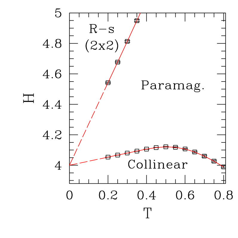
Figure 1: (Color online) Phase diagram near $H=4$, showing phase boundaries: collinear-paramagnetic, with reentrant behavior, and row-shifted [R-s] $(2\times 2)$-paramagnetic. The points are the results of extrapolating sequences of solutions of Eq. (2), obtained with fixed $T$ and variable $H$ (see text). Uncertainties are smaller than symbol sizes. Each of the dashed lines at $T<0.2$ is the continuation of the best-fitting straight line joining points at $0.2\leq T\leq 0.4$, on the respective phase boundary.

In Figure 1 we show our results for the low-temperature part of the phase diagram, near $H=4$. Although numerical convergence difficulties prevented us from reaching $T<0.2$ for the largest strip widths, we managed to evince clearly-defined trends followed along both critical lines, on their approach to $T=0$. Below $T=0.4$, both the collinear-paramagnetic and row-shifted $(2\times 2)$-paramagnetic boundaries are, to a very good approximation, straight, and pointing towards $(T,H)=(0,4)$ with respective slopes $0.267(1)$ and $2.713(5)$. Concurring with Ref. yl09, , it appears very unlikely that an $XY$-like region, or a bicritical point at $T>0$, is present. Instead, all indications from our results are consistent with both critical lines joining at a single bicritical point at $T=0$. Additionally, we found the maximum of the reentrance on the collinear-paramagnetic phase boundary to be $H=4.121(2)$ at $T=0.5$. At $T=0.7$ we estimate $H=4.060(6)$. These are in rather good agreement with the respective values $H=4.07(2)$ and $4.052(7)$, quoted in Ref. yl09, .

Near $H=0$, the phase boundary has the expected parabolic shape k87 ; dq09b :

$$T_{c}(H)=T_{c}(0)-a\,H^{2}\ \ \quad(H\to 0)\ ,$$ (15)

where we found $a=0.0595(3)$ by fitting data corresponding to $0\leq H\leq 0.4$.

As noted previously in Ref. akg84, and above, we generally found finite-size effects to be much larger for the high-field ($4\leq\ H\leq 8$) part of the phase diagram. This is illustrated in Figure 2, where finite-$N$ curves with the solutions of Eq. (2) for $N=10$ and $16$ are displayed jointly with our final extrapolation (as described above). At variance with Ref. yl09, , where $T_{c}=0.7293(7)$ is reported at $H=6$, our extrapolated value is $T_{c}(H=6)=0.589(4)$. Although alternative procedures to our ad hoc parabolic extrapolations against $N^{-2}$ can certainly be devised, it must be noted that for this same field intensity the solution of Eq. (2) is $T^{\ast}_{N}=0.706$ already for $N=10$, and decreases systematically with increasing $N$.

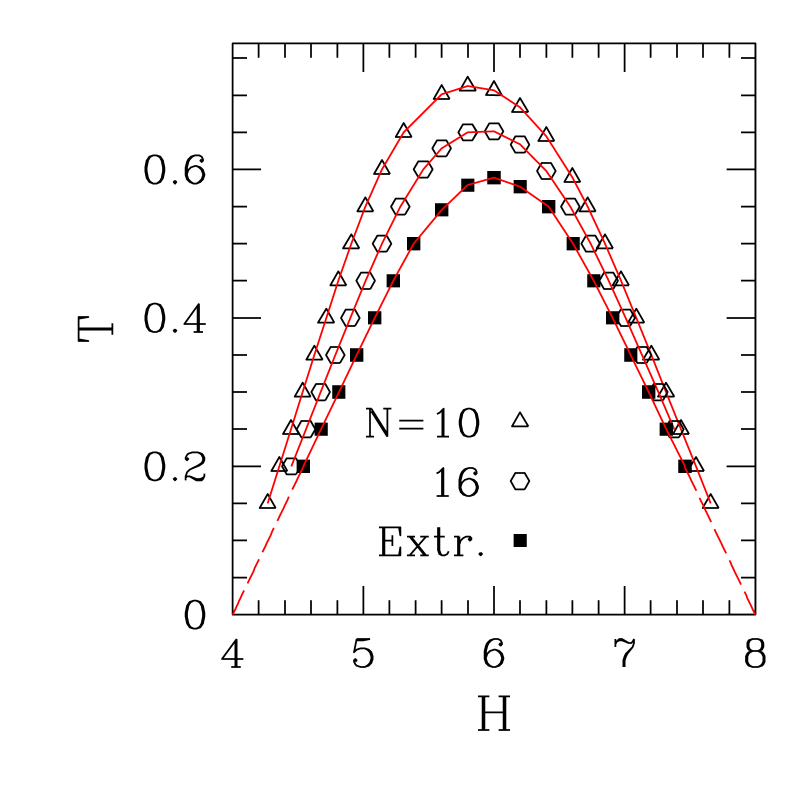
Figure 2: (Color online) Phase diagram for high fields $4\leq H\leq 8$, showing row-shifted [R-s] $(2\times 2)$-paramagnetic phase boundary: finite-$N$ solutions of Eq. (2) for $N=10$ and $16$, and results of extrapolation of $N=10-16$ curves (see text). Uncertainties in the latter are smaller than symbol sizes. Each of the dashed lines at $T<0.2$ is the continuation of the best-fitting straight line joining points at $0.2\leq T\leq 0.4$, on the respective section of the extrapolated phase boundary.

At $(T,H)=(0,8)$, the initial slope $S=(dH_{c}/dT)_{T=0}$ of the critical curve gives an estimate of the reduced critical chemical potential $\mu/k_{B}T_{c}$ for the hard-square lattice gas with first- and second-neighbor exclusion, via $\mu/k_{B}T_{c}=-2S$ akg84 . Our result for the chemical potential is $5.42$, to be compared with $4.70$ akg84 , and $4.91$ slotte . This may indicate that our extrapolation procedures slightly underestimate the extent of the row-shifted $(2\times 2)$ phase.

Figure 3 shows our results for $\eta$ and $c$ along the extrapolated location of the collinear-paramagnetic border, parametrized by $T$. These are obtained from Eqs. (4) and (9), respectively. In part (a), comparison between $N=10$ estimates and the final $N\to\infty$ extrapolation illustrates that residual finite-size effects contribute towards overestimating the exponent $\eta$, for all $0<T\lesssim 1.78$ (the approximate point where all finite-$N$ curves cross). On the other hand, for higher $T$ the finite-size corrections change sign. The extrapolated $\eta\times T$ curve is to a large extent horizontal, near both the low- and high-temperature ends of the phase boundary. We estimate $\eta=0.2476(3)$ for $T\leq 0.5$, and $\eta=0.2342(3)$ for $T\geq 1.3$. In the intermediate region there is a crossover which becomes rather sharp around $T=0.8$, at the upper end of the reentrant part of the phase diagram. The conformal-anomaly estimates in part (b) show the same behavior found for $H=0$ in Section III.1, and in Ref. kalz11, , in that they are always slightly above unity. Similarly to the $H=0$ case, we also found that, upon fitting free-energy data in the range $[N_{\rm min},20]$, the estimates of $c$ always decrease upon increasing $N_{\rm min}$. Thus, an interpretation of the present results as consistent with $c=1$, albeit affected by strong crossover effects, seems credible.

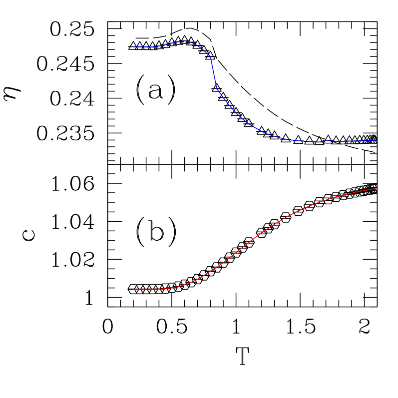
Figure 3: (Color online) (a) Decay-of-correlations exponent $\eta$ and (b) conformal anomaly $c$, calculated along the extrapolated collinear-paramagnetic phase boundary. In (a), the dashed line gives estimates of $\eta$ from strips of width $N=10$ sites, while points are extrapolations from sets of finite-$N$ estimates, $N=14-20$. In (b), values of $c$ are estimated from quadratic fits of free-energy data against $N^{-2}$ for $N=14-20$. Uncertainties are smaller than symbol sizes.

We evaluated critical magnetizations, as given by Eq. (14), along the collinear-paramagnetic phase boundary. Our calculations did not converge for $T<0.75$, which approximately coincides with the reentrant region. Thus, for the part of the critical boundary where we managed to produce estimates of $\beta/\nu$, there is a one-to-one correspondence between field and temperature. Our results are shown in Figure 4, parametrized by $H$. This way, it is easier to follow the evolution of quantities for low fields than if we used $T$ for the horizontal axis, because of the parabolic shape assumed by the critical curve in that region. One sees that the quality of fits generally deteriorates as $H$ increases; the shallow dip around $H\approx 1.5$ is possibly related to slight inaccuracies in the determination of the extrapolated critical line in that region. A more persistent trend is that towards increasing values for larger $H$. We interpret this as signalling the onset of the physical effects which give rise to reentrant behavior for even larger fields. Indeed, a plausible explanation for the reentrance is, to quote Ref. yl09, , ‘the appearance of $(2\times 2)$ "clusters" that help to sustain the [ collinear ] order at low temperatures even when the external field is slightly bigger than $4$’. This sort of cluster is not taken into account in our column-magnetization calculations, see Eq. (14). We also know that the general effect of neglecting relevant contributions to the magnetization is to increase the apparent value of $\beta/\nu$; for instance, if $M_{\rm u}$ is discarded in Eq. (14), the estimate of $\beta/\nu$ at $T=2.0820$, $H=0$ goes from $0.120(2)$ to $0.135(2)$. According to this interpretation, for $H\simeq 2.5$ or thereabouts, $(2\times 2)$ configurations which are locally energetically favorable start contributing to ordering in the $N\to\infty$ limit, but are not captured in the scheme of Eq. (14). With decreasing $T$ and increasing $H$, the effect of such configurations becomes more relevant, providing a mechanism through which the apparent exponent increases, although the real one, we conjecture, possibly increases a little but stays slightly below $1/8$. This would be in line with the behavior of $\eta$, depicted in part (a) of Figure 3.

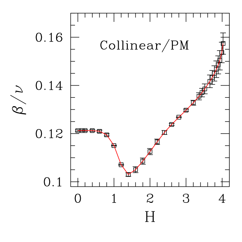
Figure 4: (Color online) Finite-size magnetization exponent $\beta/\nu$ along collinear-paramagnetic (PM) phase boundary. The range of fields, $0\leq H\leq 4.027$, on the horizontal axis corresponds, respectively, to $2.0820\geq T\geq 0.75$ (see text). Each point is the result of fitting finite-size data in the range $12\leq N\leq 20$ to a single-power law, $\langle M^{2}\rangle^{1/2}\sim N^{1-\beta/\nu}$. See Eqs. (8) and (14).

Calculation of the thermal exponent $y_{T}$ via Eq. (3) in the reentrant region gave negative values, an artifact already noticed in Refs. kkg83, ; akg84, . However, evaluation of critical finite-size susceptibilities at $T=0.35$ gives $\gamma/\nu$ in the range $1.71-1.80$, depending on the details of corrections to scaling assumed for data fitting. Although lacking in accuracy, this range of values is broadly consistent both with the corresponding $\eta$ estimate, and with the hypothesis that critical behavior obeys weak universality all along the collinear-paramagnetic critical line.

Turning now to the high-field part of the phase diagram, we illustrate in Figure 5 our results for $\eta$ along the approximate critical lines, the latter obtained by solving Eq. (2) for $N=10-16$. The curve for $N=12$ corresponds to that shown in Figure 2 of Ref. akg84, .

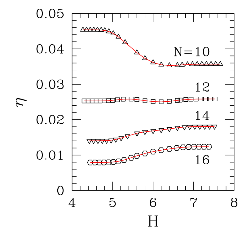
Figure 5: (Color online) Decay-of-correlations exponent $\eta$, evaluated via Eq. (4), along approximate row-shifted $(2\times 2)$-paramagnetic transition lines, obtained by solving Eq. (2) for $N$ as indicated, for high fields $4\leq H\leq 8$.

By comparing the evolution of $\eta$ along the approximate critical lines with the evolution of the lines themselves against increasing $N$, shown in Figure 2, one anticipates that calculating $\eta$ on the extrapolated phase boundary will give results very close to zero, or even slightly negative. Indeed, this was what we found. It would appear that this is at least partly because our extrapolation procedures underestimate the extent of the row-shifted $(2\times 2)$ phase. Evaluation of $c$ along the extrapolated critical line also gave physically inconsistent results.

Even though we are not able to produce numerically accurate estimates of $\eta$ for the high-field part of the phase diagram, the gist of the results shown in Figure 5 is that this must be below $0.01$, and possibly even zero. We return to this point in the next Section.

IV Discussion and Conclusions

For the model described by Eq. (1), with $J_{2}=1$, we have established a physical picture for the collinear-paramagnetic phase boundary, which is consistent with continuously-varying exponents along the critical line. Together with various pieces of numerical evidence, collected at selected points, overall support for this is given by the conformal anomaly results depicted in part (b) of Figure 3.

There is also clear evidence that such continuously-varying exponents satisfy, at least approximately, a weak-universality scenario s74 . However, as shown for the exponent $\eta$ in part (a) of Figure 3, our results indicate small but consistent deviations from the corresponding Ising values.

Furthermore, such deviations are internally consistent, in the sense that both $\eta$ and $\beta/\nu$ take on values lower than the Ising ones, while $\gamma/\nu$ is always found to be higher than the Ising result. For $\beta/\nu$, the apparent reversal of this trend found for $H\gtrsim 2.5$ has been explained in Section III.2, as a likely effect of the same sort of locally stable $(2\times 2)$ configurations which, at lower $T$ and higher $H$, become significant enough to induce reentrant behavior.

Notwithstanding the compensation just referred to, our estimates of $(\gamma/\nu)+\eta$ in general exceed $2$, though never by more than $2-3$ times the respective (combined) error bar. However, it must be recalled that here $\gamma/\nu$ is essentially one order of magnitude larger than $\eta$, and both quantities have similar relative uncertainties, thus the calculated combined uncertainty is practically only that associated with $\gamma/\nu$. In such circumstances, the apparent violation of a fundamental scaling relation reflects the fact that the relative uncertainty in $\gamma/\nu$ was estimated as $\approx 2$ parts in $10^{3}$. Had this been doubled, all the basic conclusions from this work would still stand, and the mismatch would be essentially lost within the revised error bars.

Returning to $\eta$ as displayed in part (a) of Figure 3, the small but consistent shift between the high- and low-$T$ approximately constant values [ respectively, $0.2342(3)$ and $0.2476(3)\,$] indicates a crossover between two distinct weak-universality classes. Such small variations could probably be accounted for in the context of compactified boson theory dif97 ; k88 , in which continuously-varying critical indices are put in direct correspondence with the (also continuously-varying) radius $R$ associated with the underlying field theory.

In general, both for $H=0$ and $H\neq 0$ (the latter, along the collinear-paramagnetic critical line) our results for the location of critical points, and exponents such as $y_{T}$, $\gamma/\nu$, and $\beta/\nu$, are mostly compatible, within error bars, with estimates available in the literature. On the other hand, for the row-shifted ($2\times 2)$-paramagnetic phase boundary at high fields, we have found a discrepancy of some $19\%$ between our estimate and that given in Ref. yl09, , for the highest transition temperature at $H=6$. Even allowing for the (rather plausible) likelihood that our extrapolation procedures underestimate the extent of the ordered phase, for PRG with the largest size available ($N=16$) one has $T_{c}(H=6)=0.651$, already $11\%$ below $T_{c}(H=6)=0.7293(7)$ quoted in Ref. yl09, . At this point, such discrepancy remains unexplained.

We have not succeeded in gathering as much information regarding critical properties of the row-shifted ($2\times 2)$-paramagnetic boundary line, as we did for its collinear-paramagnetic counterpart. However, the behavior of $\eta$ illustrated in Figure 5 reminds one of the low-temperature behavior of the two-dimensional $XY$ model. Indeed, with $T_{KT}$ being the upper limit of the Kosterliz-Thouless critical phase, the exponent $\eta$ of the $XY$ model grows smoothly and monotonically from $\eta=0$ at $T=0$ to $1/4$ at $T_{KT}$ (with most of the increase confined to higher $T$: at $T=0.5\,T_{KT}$, $\eta\approx 0.05$) bsp02 . So the very low values of $\eta$ found in the present case may, or may not, indicate the presence of incipient $XY$-like behavior along at least part of the high-field critical line.

- (1) G. Misguich and C. Lhuillier, in Frustrated Spin Systems, edited by H. T. Diep (World Scientific, Singapore, 2005).
- (2) J. T. Chalker, in Introduction to Frustrated Magnetism: Materials, Experiment, Theory, edited by C. Lacroix, P. Mendels, and F. Mila, Springer Series in Solid-State Sciences vol. 164 (Springer, Berlin, 2011).
- (3) Junqi Yin and D. P. Landau, Phys. Rev. E80, 051117 (2009).
- (4) A. Kalz, A. Honecker, S. Fuchs, and T. Pruschke, Eur. Phys. J. B 65, 533 (2008).
- (5) M. P. Nightingale, in Finite Size Scaling and Numerical Simulations of Statistical Systems, edited by V. Privman (World Scientific, Singapore, 1990).
- (6) M. N. Barber, in Phase Transitions and Critical Phenomena, edited by C. Domb and J. L. Lebowitz (Academic, New York, 1983), Vol. 8.
- (7) J. L. Cardy, in Phase Transitions and Critical Phenomena, edited by C. Domb and J. L. Lebowitz (Academic, New York, 1987), Vol. 11.
- (8) H. W. J. Blöte, J. L. Cardy, and M. P. Nightingale, Phys. Rev. Lett. 56, 742 (1986).
- (9) J. L. Cardy, J. Phys. A 17, L385 (1984).
- (10) K. Kaski, W. Kinzel, and J. D. Gunton, Phys. Rev. B27, 6777 (1983).
- (11) J. Amar, K. Kaski, and J. D. Gunton, Phys. Rev. B29, 1462 (1984).
- (12) M. P. Nightingale and H. W. J. Blöte, Physica A 251, 211 (1998).
- (13) B. Derrida and L. de Seze, J. Phys. (Paris) 43, 475 (1982).
- (14) M. P. Nightingale and H. W. J. Blöte, J. Phys. A 15, L33 (1983).
- (15) V. Privman and M.E. Fisher, J. Phys. A 16, L295 (1983).
- (16) T. W. Burkhardt and I. Guim, J. Phys. A 18, L25 (1985).
- (17) T. W. Burkhardt and I. Guim, J. Phys. A 18, L33 (1985).
- (18) H. W. J. Blöte and M. P. Nightingale, Physica A 112, 405 (1982).
- (19) H. W. J. Blöte and M. P. Nightingale, Physica A 134, 274 (1985).
- (20) M. P. Nightingale and H. W. J. Blöte, J. Phys. A 16, L657 (1983).
- (21) C. J. Hamer, J. Phys. A 15, L675 (1982).
- (22) J. L. Cardy, J. Phys. A 20, L891 (1987).
- (23) P. di Francesco, P. Mathieu, and D. Sénéchal, Conformal Field Theory (Springer-Verlag, New York, 1997).
- (24) A. Kalz, A. Honecker, and M. Moliner, arXiv:1105.4836 (2011).
- (25) M. Hasenbusch, F. Parisen Toldin, A. Pelissetto, and E. Vicari, Phys. Rev. E77, 051115 (2008).
- (26) S. L. A. de Queiroz, Phys. Rev. B79, 174408 (2009).
- (27) A. Malakis, P. Kalozoumis, and N. Tyraskis, Eur. Phys. J. B 50, 63 (2006).
- (28) J. L. Monroe and S.-Y. Kim, Phys. Rev. E76, 021123 (2007).
- (29) S.-Y. Kim, Phys. Rev. E81, 031120 (2010).
- (30) M. Suzuki, Prog. Theor. Phys. 51, 1992 (1974).
- (31) K. Binder and D. P. Landau, Phys. Rev. B21, 1941 (1980).
- (32) M. Kaufman, Phys. Rev. B36, 3697 (1987).
- (33) S. L. A. de Queiroz, Phys. Rev. E80, 041125 (2009).
- (34) P. A. Slotte, J. Phys. C 16, 2935 (1983).
- (35) M. Karowski, Nucl. Phys. B300, 473 (1988).
- (36) B. Berche, A. I. F. Sanchez, and R. Paredes, Europhys. Lett. 60, 539 (2002).