Percolation and Schramm-Loewner evolution in the 2D random-field Ising model

Abstract

The presence of random fields is well known to destroy ferromagnetic order in Ising systems in two dimensions. When the system is placed in a sufficiently strong external field, however, the size of clusters of like spins diverges. There is evidence that this percolation transition is in the universality class of standard site percolation. It has been claimed that, for small disorder, a similar percolation phenomenon also occurs in zero external field. Using exact algorithms, we study ground states of large samples and find little evidence for a transition at zero external field. Nevertheless, for sufficiently small random field strengths, there is an extended region of the phase diagram, where finite samples are indistinguishable from a critical percolating system. In this regime we examine ground-state domain walls, finding strong evidence that they are conformally invariant and satisfy Schramm-Loewner evolution ($SLE_{\kappa}$) with parameter $\kappa=6$. These results add support to the hope that at least some aspects of systems with quenched disorder might be ultimately studied with the techniques of SLE and conformal field theory.

The random field Ising model (RFIM) is one of the earliest studied and simplest disordered systems showing non-trivial and glassy behavior [1, 2]. It has a number of important realizations in nature, including diluted antiferromagnets in a field and binary liquids in porous media [2]. Through its long history, researchers have managed to gain a reasonable understanding of the critical behavior, although this progress has been neither straight nor smooth, and many questions remain unanswered [2]. It is known, for example, that the RFIM in two dimensions (2D) lacks ferromagnetic order [3, 4]. Even at zero temperature it remains in the paramagnetic state for non-zero disorder. Numerical ground-state calculations have shown, however, that even in the absence of a thermodynamic transition there exists a geometric transition at which the size of the spin clusters diverges in a manner bearing many similarities to classical site percolation [5, 6]. While this transition is rather clearly established in the presence of an external field, it has been argued that a similar percolation phenomenon can also be observed in the absence of an external field for sufficiently small disorder [6, 7]. Here, we re-investigate the zero-field behavior with large scale ground-state calculations, focusing on the possible percolation phenomenon.

The observed relations to classical site percolation at this (non-zero or zero field) geometrical transition motivate further questions of how far the similarities go. Interfaces in two-dimensional percolation satisfy Schramm-Loewner evolution (SLE) [8, 9], but this property relies on conformal invariance which is not conserved in the presence of disorder. Recently, however, there have been suggestions that the domain walls of certain other disordered systems satisfy SLE. This intriguing possibility implies that conformal invariance, broken by disorder, is restored, at least at criticality where relevant length scales diverge.

Schramm-Loewner evolution is a method for constructing a statistical ensemble of curves in the plane from one-dimensional Brownian motion, thus classifying curves with only one parameter, the diffusion constant $\kappa$ [10]. Characteristic interfaces in many physical systems have been shown (in some cases rigorously) to satisfy SLE_κ. These include percolation ($\kappa=6$), self avoiding walks ($\kappa=4/3$), as well as spin cluster boundaries ($\kappa=3$) and Fortuin-Kasteleyn cluster boundaries ($\kappa=16/3$) in the Ising model. A number of numerical studies have found interfaces in certain disordered systems consistent with SLE, in particular the 2D Ising spin glass[11, 12], the Potts model on dynamical triangulations [13], the random bond Potts model [14], and the disordered solid-on-solid model [15]. Here we extend this list to include the 2D random field Ising model.

In Sec. 1 we introduce the RFIM and Schramm-Loewner evolution in more detail, and discuss the approach used here for determining ground states of large samples. Section 2 is devoted to an investigation of the critical behavior of the RFIM near the geometric transition, focusing on the behavior in zero external field for small disorder. In Sec. 3, we report the results of our tests of the correspondence between interfaces in the RFIM and Brownian motion implied by SLE.

1 The model and method

We consider the random field Ising model in two dimensions with Hamiltonian

$$\mathcal{H}=-J\sum_{\langle i,j\rangle}s_{i}s_{j}-\sum_{i}h_{i}s_{i}.$$ (1)

Here, the spins $s_{i}=\pm 1$ are located on the sites of a square lattice and interact ferromagnetically with nearest neighbors. The local fields $h_{i}$ are quenched random variables drawn from a normal distribution with mean $H$ and standard deviation $\Delta$. Since, at zero temperature, only the ratio $J/\Delta$ is relevant, we take $J=1$ for simplicity. The spin-spin interaction $J$ induces a correlation between the spins resulting in spin clusters which are compact up to a length $\xi_{b}$. Above this scale the clusters are fractal objects, the magnetization is zero and the system is paramagnetic. As the randomness $\Delta$ is decreased, the breakup length $\xi_{b}$ increases. At and above three dimensions $\xi_{b}$ diverges at the thermodynamic phase transition, below which the system is ferromagnetic. In two dimensions no thermodynamic phase transition exists, and $\xi_{b}$ diverges only at $\Delta=0$. It has been argued that, for $H=0$, the breakup length scale $\xi_{b}$ increases with decreasing $\Delta$ as [3]

$$\xi_{b}\sim e^{A/\Delta^{2}}.$$ (2)

Though there is no thermodynamic transition in 2D, the linear extent of the largest clusters diverges for sufficiently large $H$. In most aspects, this divergence appears to be consistent with standard site percolation [5, 6, 7]. It has been suggested that the divergence occurs even at $H=0$ if $\Delta$ is below a critical value [5, 7]. It is the characteristics of clusters of aligned spins and their boundaries at this geometric transition which we focus on in this study.

We restrict our investigation to ground-state spin configurations, which can be efficiently constructed through a mapping to the well known minimum cut (or maximum flow) problem in graph theory [16, 17]. Consider a directed graph with $N+2$ vertices, and edges $(i,j)$ furnished with weights $c_{ij}$. The minimum $(s,t)$ cut is given by a subset of the edges of the graph, whose removal disconnects vertices $s$ and $t$, such that the sum of the weights of the cut edges is minimal. Using the variables $x_{i}$, which are 1 if vertex $i$ is connected to $s$ and 0 otherwise, the total weight of a cut can be represented as

$$C(\{\mathbf{x}\})=\sum_{i,j=1}^{N}x_{i}(1-x_{j})c_{ij}.$$ (3)

With the identification of $x_{i}$ with spin variables (excepting the vertices $s$ and $t$), and an appropriate choice of the weights $c_{ij}$, this function can be made to precisely match the RFIM Hamiltonian (1). The minimum cut separating the graph into vertices connected to $s$ and vertices connected to $t$ gives the minimum-energy way of cutting the RFIM lattice into clusters of up and down spins, and thus corresponds to the ground state of equation 1. The choice for the edge weights is, for $i\notin(s,t)$

$$c_{ij}=\left\{\begin{array}[]{ll}0,&i\geq j\\ 4J,&\mathrm{else}\end{array}\right..$$ (4)

For the edges connecting the “spin” vertices to $s$ and $t$, the result is given in terms of the quantity $u_{i}=-h_{i}-\frac{1}{2}\sum_{j}(c_{ij}-c_{ji})$ as

$$c_{si}=\left\{\begin{array}[]{ll}0,&u_{i}>0\\ -u_{i},&\mathrm{else}\end{array}\right.,\;\;\;c_{it}=\left\{\begin{array}[]{ll}u_{i},&u_{i}>0\\ 0,&\mathrm{else}\end{array}\right..$$ (5)

$c_{is}$ and $c_{ti}$ are taken to be zero for all $i$. Here, we use a fast algorithm for solving the minimum cut problem based on the idea of “augmenting paths”[18, 19]. The worst case scenario for the running time of this algorithm is an unimpressive $O(N^{3})$ (or more generally $V^{2}E$ where $V$ is the number of vertices and $E$ is the number of edges), however, the algorithm was designed to optimize the typical case. The optimization was carried out for vision and image analysis problems, but even for the graph structure corresponding to the RFIM ground state calculation the running time is proportional to $N$ for the samples considered here. In practice, the maximum system size is limited more by computer memory constraints than by time.

Schramm-Loewner evolutions are defined in terms of a family $g_{t}$ of conformal maps which take, formally, the upper half plane minus the curve $\gamma_{t}$ (parametrized by “time” $t$) to the upper half plane, $g_{t}:\mathbb{H}\setminus\gamma_{t}\to\mathbb{H}$. This map can be defined (using complex notation and suitable normalization) in terms of the differential equation

$$\frac{\partial g_{t}(z)}{\partial t}=\frac{2}{g_{t}(z)-\xi_{t}}$$ (6)

where $\xi_{t}$ is the unique driving function for the curve $\gamma_{t}$. If the curve (or the process generating the curve) satisfies SLE_κ, then $\xi_{t}$ will be a Brownian motion with zero mean and variance $\kappa t$. Numerically, rather than solving the differential equation, the map $g_{t}$ is instead pictured as a series of maps $g_{i}$ which iteratively remove a small section from the beginning of the curve. To calculate the driving function from a given curve, the incremental map $g_{i}$ is approximated using a vertical slit map [20]

$$g_{i}(z)=i\sqrt{-(z-\xi_{i})^{2}-4\Delta t_{i}}+\xi_{i}.$$ (7)

The parameters $\xi_{i}$ and $\Delta t_{i}$ are determined from the coordinates of the curve segment to be removed through the relations $\xi_{i}=x_{i,i-1}$ and $\Delta t_{i}=y_{i,i-1}^{2}/4$. More specifically, $x_{i,i-1}$ and $y_{i,i-1}$ are the coordinates of the $i$’th segment of the curve after undergoing the $i-1$ successive maps $g_{i-1}\circ\ldots\circ g_{1}$. The parameter $\xi_{i}$ is the value of the driving function $\xi_{t}$ sampled at time $t_{i}=\sum_{j\leq i}\Delta t_{j}$. The complex square root in equation 7 is calculated, as usual, with the branch cut along the negative real axis.

This is an iterative process in which the coordinates of the interface are successively updated for each step, and thus the computational complexity is $O(L_{I}^{2})$ where $L_{I}$ is the length of the interface. If $L_{I}$ grows like $\sim N^{d_{f}/2}$ (with $d_{f}=7/4$ expected for percolation) in the number of spins $N$, the resulting computational complexity is $O(N^{7/4})$, which is significantly slower than the ground-state calculation which is $O(N)$ on average. We use a fast implementation of this “zipper” algorithm [21], in which blocks of multiple slit maps are approximated by a Laurent series. Treating blocked maps in one step dramatically speeds up the calculation such that it scales on average as $L_{I}^{1.3}$. The loss in accuracy from the approximation is minimal.

If the driving function $\xi_{t}$ can be shown to be Brownian motion then the curves satisfy SLE_κ. In practice, the finite size of the lattice and the zipper algorithm introduces correlations between the increments of $\xi_{i}$ and in their associated time values $t_{i}$. In particular the distribution of time steps $t_{i}-t_{i-1}$ is highly non-trivial and has significant correlations. However, it should be emphasized that correlations in the times $t_{i}$ at which $\xi_{t}$ is sampled does not imply correlations in the underlying continuous driving function $\xi_{t}$.

2 Phase diagram and behavior at zero field

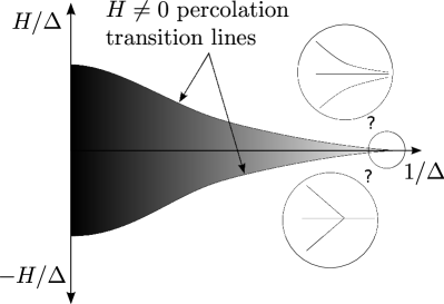
Figure 1: Schematic representation of the dependence of the location $H_{c}$ of the percolation transition on the random-field strength $\Delta$. For $H<H_{c}$ the spin clusters have finite extent. For $H\geq H_{c}$ there exists at least one infinite cluster.

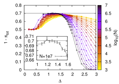
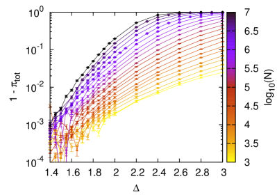
Figure 2: Crossing probabilities for spin clusters of the 2D RFIM on rectangular domains of aspect ratio $e^{-2/5}$ for a number of system sizes $N=e^{-2/5}L^{2}$ at $H=0$. Top panel: probability of crossing of clusters of up spins in the vertical direction. For $\Delta$ decreasing from infinity, the crossing probability approaches the exact percolation crossing value [22], indicated by the horizontal line. At very small disorder, the breakup length $\xi_{b}$ is larger than the system size and the systems are effectively ferromagnetic. Inset: enlarged view of the plateau region for the largest system size. The bottom panel shows $1-\pi_{tot}$, the total crossing probability. If there was a transition at $H=0$, the lines would have to cross around the transition point.

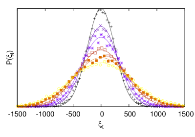
Figure 3: Distribution of the random walk at several different “times” $t$ as extracted from the RFIM interfaces at $\Delta=1.65$. The lines are normal distributions with zero mean and variance $\kappa t$ with $\kappa=6$.

For very large disorder, $\Delta\gg Jz$, where $z$ is the lattice coordination number, the interactions between the spins play no role and the system reduces, trivially, to the classical site percolation model. Each spin is determined solely by the independent random variable $h_{i}$. Identifying spin up with “site occupation”, the site occupation probability $p$ is simply the probability for $h_{i}$ to be positive: $p=\frac{1}{2}\mathrm{erfc}\{-H/(\sqrt{2}\Delta)\}$. For smaller disorder the spin-spin interaction of the RFIM complicates the analogy with percolation. However, it has been demonstrated that there exists a line of critical external fields $H_{c}(\Delta)$, as pictured schematically in Fig. 1, for which observables like the crossing probability and the fractal dimension of the spin clusters maintain the percolation values [6].

For very large disorder the line of critical external fields is found from the critical site percolation probability $p_{c}$ ($p_{c}\approx 0.5927$ for the square lattice)

$$H_{c}(\Delta\gg z)\approx-\Delta\sqrt{2}\mathrm{erfc}^{-1}\{2p_{c}\}.$$ (8)

For small disorder the behavior is less well understood. $H_{c}(\Delta)$ decreases as $\Delta$ decreases, approaching the limiting value $H_{c}(\Delta=0)=0$. It has been claimed [6, 7] that at a finite disorder strength, $\Delta_{c}\approx 1.65(5)$, the curve becomes identically zero $H_{c}(\Delta<\Delta_{c})=0$, cf. Fig. 1. We tested this claim by looking at the behavior of the system varying $\Delta$ at $H=0$. We calculated the probability that a connected cluster of up spins crosses a rectangle of aspect ratio $e^{-2/5}$ in the vertical (shorter) direction (this aspect ratio is chosen to be different from $1/2$, but the specific value is somewhat arbitrary). In the upper panel of Fig. 2, we present the results of these calculations. The crossing probability $\pi$ for large $\Delta$ is zero (as expected for a square lattice with $p_{c}>0.5$). As the disorder is decreased, $\pi$ approaches the exact percolation value, which is indicated by the horizontal line in the plot. At very small disorder, when the breakup length scale $\xi_{b}$ becomes comparable to the system size $L$, the system appears ferromagnetic and the crossing probability falls away from the plateau value.

To separate the approach to the plateau from the finite size effects we also considered another quantity, the probability $\pi_{tot}$ that there exists a connected cluster of either up or down spins crossing either horizontally or vertically. The small disorder limit of this quantity is $\pi_{tot}(\Delta\to 0)=1$ for both the onset of percolation and the ultimate ferromagnetic (and finite size) ordering. If there is a percolation transition at finite disorder ($\Delta_{c}>0$), in the thermodynamic limit $L=\infty$ the curve $\pi_{tot}(\Delta)$ will be a step function. Hence, the curves for finite systems approaching this step function will intersect at $\Delta_{c}$. As is apparent from our data for $\pi_{tot}$ shown in the lower panel of Fig. 2, such a crossing is not observed at least down to $\Delta\approx 1.45$, significantly below the previously conjectured value of $\Delta_{c}\approx 1.65$. The study of even smaller disorder strengths, while ensuring $L\gg\xi_{b}$, is preempted by the exponential growth of the breakup length $\xi_{b}$. Although it seems very unlikely that the system undergoes a true percolation phase transition for $H=0$, there exists a large plateau region in which the system appears to be at critical percolation at $H=0$, even up to very large system sizes. Presumably, this holds true even for system sizes occurring in experimental realizations of the RFIM.

3 Schramm-Loewner evolution

Finally, we tested directly the conformal mapping upon which SLE is based. We studied the statistics of $10\,000$ interfaces generated in a half disc. This geometry is used to optimally mimic the full half plane. The interface is initiated at the origin (the center of the flat edge) by two fixed spins and is considered ended when it touches the curved boundary. We find that the variance of the driving function calculated from the interfaces using the method described in Sec. 1 is $\hat{\kappa}=\langle(\xi_{t}-\langle\xi_{t}\rangle)^{2}\rangle/t=6.09\pm 0.09$, and the normalized mean is $\hat{\xi}=\langle\xi_{t}\rangle/\sqrt{\hat{\kappa}t}=0.01\pm 0.01$. The agreement with SLE is good, but is only expected to be perfect at criticality. The difference from the expected percolation value $\kappa=6$ which is perhaps just visible here is due to the calculations being carried out at $\Delta=1.65$. The position distribution of the resulting stochastic process at several fixed times is shown in Fig. 3 along with curves representing the expectations for a perfect random walk.

We have focused here on the case of zero external field, where we have shown, using significantly larger system sizes than had been accessible before, that there is no percolation phase transition for $H=0$, at least down to $\Delta=1.45$. Due to the fact, however, that the percolation transition line comes exponentially close to $H=0$ for small random-field strengths $\Delta$ (cf. Fig. 1), there exists a plateau region where even at $H=0$ the behavior appears nearly indistinguishable from criticality. In this regime we have tested the applicability of Schramm-Loewner evolution to the RFIM and found good agreement. Further studies at non-zero external field and using an array of further tests for consistency with SLE confirm this result [23].

The authors acknowledge computer time provided by NIC Jülich under grant No. hmz18 and funding by the DFG through the Emmy Noether Program under contract No. WE4425/1-1.

References

- Binder and Young [1986] K. Binder, A. P. Young, Spin-glasses — Experimental facts, theoretical concepts, and open questions, Rev. Mod. Phys. 58 (1986) 801–976.
- Nattermann [1997] T. Nattermann, Theory of the random field Ising model, in: A. P. Young (Ed.), Spin Glasses and Random Fields, World Scientific, 1997, p. 277.
- Binder [1983] K. Binder, Random-field induced interface widths in Ising systems, Z. Phys. B 50 (1983) 343–352.
- Aizenman and Wehr [1989] M. Aizenman, J. Wehr, Rounding of first-order phase transitions in systems with quenched disorder, Phys. Rev. Lett. 62 (1989) 2503.
- Seppälä et al. [1998] E. T. Seppälä, V. Petäjä, M. J. Alava, Disorder, order, and domain wall roughening in the two-dimensional random field Ising model, Phys. Rev. E 58 (1998) R5217–R5220.
- Seppälä and Alava [2001] E. T. Seppälä, M. J. Alava, Susceptibility and percolation in two-dimensional random field Ising magnets, Phys. Rev. E 63 (2001) 066109.
- Környei and Iglói [2007] L. Környei, F. Iglói, Geometrical clusters in two-dimensional random-field Ising models, Phys. Rev. E 75 (2007) 011131.
- Schramm [2000] O. Schramm, Scaling limits of loop-erased random walks and uniform spanning trees, Israel J. Math. 118 (2000) 221.
- Cardy [2005] J. Cardy, SLE for theoretical physicists, Ann. Phys. (N.Y.) 318 (2005) 81–118. Special Issue.
- Bauer and Bernard [2006] M. Bauer, D. Bernard, 2D growth processes: SLE and Loewner chains, Phys. Rep. 432 (2006) 115–221.
- Amoruso et al. [2006] C. Amoruso, A. K. Hartmann, M. B. Hastings, M. A. Moore, Conformal invariance and stochastic Loewner evolution processes in two-dimensional Ising spin glasses, Phys. Rev. Lett. 97 (2006) 267202.
- Bernard et al. [2007] D. Bernard, P. Le Doussal, A. A. Middleton, Possible description of domain walls in two-dimensional spin glasses by stochastic Loewner evolutions, Phys. Rev. B 76 (2007) 020403.
- Weigel and Janke [2006] M. Weigel, W. Janke, Geometric and stochastic clusters of gravitating Potts models, Phys. Lett. B 639 (2006) 373.
- Jacobsen et al. [2009] J. L. Jacobsen, P. Le Doussal, M. Picco, R. Santachiara, K. J. Wiese, Critical interfaces in the random-bond Potts model, Phys. Rev. Lett. 102 (2009) 070601.
- Schwarz et al. [2009] K. Schwarz, A. Karrenbauer, G. Schehr, H. Rieger, Domain walls and chaos in the disordered SOS model, J. Stat. Mech. (2009) P08022.
- Anglès d’Auriac et al. [1985] J. C. Anglès d’Auriac, M. Preissmann, R. Rammal, The random field Ising model — Algorithmic complexity and phase transition, J. Physique Lett. 46 (1985) L173–L180.
- Hartmann and Rieger [2002] A. K. Hartmann, H. Rieger, Optimization Algorithms in Physics, Wiley-VCH, Berlin, 2002.
- Kolmogorov [2003] V. Kolmogorov, Graph Based Algorithms for Scene Reconstruction from Two or More Views, Ph.D. thesis, Cornell University, Ithaca, NY, 2003.
- Boykov and Kolmogorov [2004] Y. Boykov, V. Kolmogorov, An experimental comparison of min-cut/max-flow algorithms for energy minimization in vision, IEEE Trans. Pattern Anal. Mach. Intell. 26 (2004) 1124–1137.
- Kennedy [2009] T. Kennedy, Numerical computations for the Schramm-Loewner evolution, J. Stat. Phys. 137 (2009) 839–856.
- Kennedy [2007] T. Kennedy, A fast algorithm for simulating the chordal Schramm-Loewner evolution, J. Stat. Phys. 128 (2007) 1125–1137.
- Cardy [1992] J. L. Cardy, Critical percolation in finite geometries, J. Phys. A 25 (1992) L201–L206.
- Stevenson and Weigel [2010] J. D. Stevenson, M. Weigel, Domain walls and Schramm-Loewner evolution in the random-field Ising model, EPL 95 (2011) 40001.