Lepton flavor violation and non-unitary lepton mixing in low-scale type-I seesaw

Abstract

Within low-scale seesaw mechanisms, such as the inverse and linear seesaw, one expects (i) potentially large lepton flavor violation (LFV) and (ii) sizeable non-standard neutrino interactions (NSI). We consider the interplay between the magnitude of non-unitarity effects in the lepton mixing matrix, and the constraints that follow from LFV searches in the laboratory. We find that NSI parameters can be sizeable, up to percent level in some cases, while LFV rates, such as that for $\mu\to e\gamma$, lie within current limits, including the recent one set by the MEG collaboration. As a result the upcoming long baseline neutrino experiments offer a window of opportunity for complementary LFV and weak universality tests.

I Introduction

One of the biggest challenges in particle physics is to unravel the nature of the dimension five operator weinberg:1980bf responsible for generating the pattern of neutrino masses and mixings required to account for current oscillation experiments Schwetz:2011qt . Within the seesaw mechanism th-talk2 ; valle:2006vb this operator arises from the tree-level exchange of heavy messenger particles. For example, in the so-called type-I seesaw, these messengers are three $SU(3)\times SU(2)\times U(1)$ singlet right-handed neutrinos, which must be super-heavy in order to account for the observed smallness of neutrino masses. However, since singlets carry no gauge-anomaly, their number is theoretically unrestricted. Such generalized type-I seesaw schemes schechter:1980gr ; schechter:1981cv provide the theoretical basis for the formulation of the inverse seesaw mohapatra:1986bd and the linear seesaw schemes malinsky:2005bi . Both are capable of realizing the type-I seesaw mechanism at the TeV scale and, as a result, these schemes open the possibility for novel phenomena such as

1. lepton flavor and/or CP violating processes unsuppressed by neutrino masses bernabeu:1987gr ; gonzalez-garcia:1991be ; branco:1989bn ; rius:1989gk ,

2. effectively non-unitary lepton mixing matrix Antusch:2008tz ; Malinsky:2009gw ; Dev:2009aw leading to non-standard effects in neutrino propagation valle:1987gv ; nunokawa:1996tg ; Miranda:2004nb .

Both features arise from the non-trivial structure of the electroweak currents in seesaw schemes schechter:1980gr ; schechter:1981cv  .While their expected magnitude is negligible within the standard type-I seesaw, it can be sizeable in low-scale seesaw mechanisms.

In this paper we analyse quantitatively the interplay between these two classes of processes. More precisely we define reference parameters describing the typical magnitude of non-standard neutrino propagation effects and compare them with the constraints which arise from the searches for lepton flavor violating (LFV) processes nakamura2010review ; :2011ch ; Ahmed:2001eh . For definiteness we focus on two simple realizations of low-scale seesaw, namely the inverse and linear seesaw schemes. Non-unitarity effects may also arise from the charged lepton sector Ibanez:2009du , leading also to lepton flavor violation.

We find that unitarity violation effects in neutrino propagation at the percent level are consistent with the current bounds from lepton flavor violation searches. Therefore their search at upcoming neutrino oscillation facilities bandyopadhyay:2007kx opens a window of opportunity to probe for new effects beyond the standard model.

The paper is organized as follows: in section II we review the type-I seesaw mechanisms, first the high-scale and then the low-scale linear and inverse seesaw realizations, fixing the notation and giving general expressions for the unitarity violating parameters; in section III we study the analytical expressions relating LFV decay branching ratios with the non-standard pieces of the general seesaw lepton mixing matrix characterizing inverse and linear seesaw schemes; in section IV we describe the parameters used in our numerical analysis, and in Sec. V we present our numerical results, both for normal and inverse neutrino mass hierarchies. Finally we give our conclusions.

II High and low-scale seesaw mechanisms

The smallness of neutrino mass with respect to that of charged fermions can be naturally accounted for within the seesaw mechanism, in which the Standard Model is extended with extra $SU(3)\times SU(2)\times U(1)$ singlets th-talk2 ; valle:2006vb . In this case the resulting neutrino mass matrix in general is a $N\times N$ matrix with $N>3$. Here we analyse the structure of this matrix in the high and low-scale type-I seesaw schemes.

II.1 The standard type-I seesaw

In general seesaw schemes the neutrino mass matrix $M_{\nu}$ can be decomposed in sub-blocks involving the standard as well as singlet neutrinos as follows

$$M_{\nu}=\left(\begin{array}[]{cc}M_{1}&M_{D}\\ M_{D}^{T}&M_{2}\end{array}\right).$$ (1)

in the basis $\nu,~{}\nu^{c}$, where the blocks $M_{1}\equiv M_{L}$ and $M_{2}\equiv M_{R}$ are symmetric matrices. Though the number of singlets is arbitrary, here we take an equal number of SU(2) doublets and singlets, and consider the simplest type-I seesaw, where no Higgs triplet is present, so the upper left sub-matrix $M_{1}=0$ in Eq. (1) schechter:1980gr  . Neutrino masses arise by diagonalizing the matrix of Eq. (1),

$$U^{T}\,M_{\nu}\,U=\text{real, diagonal}.$$ (2)

through the transformation $U$ connecting the weak states to the light and heavy mass eigenstates. We adopt a polar decomposition for $U$ where

$$U=\exp(iH)\cdot V\,,\qquad H=\left(\begin{array}[]{cc}0&S\\ S^{\dagger}&0\end{array}\right),\qquad V=\left(\begin{array}[]{cc}V_{1}&0\\ 0&V_{2}\end{array}\right).$$ (3)

so we have a power series expansion for Eq. (3) given as schechter:1981cv :

$$U=\left(\begin{array}[]{cc}\left(I-\frac{1}{2}S\,S^{\dagger}\right)\,V_{1}&i\,S\,V_{2}\\ i\,S\,V_{1}&\left(I-\frac{1}{2}S^{\dagger}\,S\right)\,V_{2}\end{array}\right)+O(\epsilon^{3})\equiv\left(\begin{array}[]{cc}U_{a}&U_{b}\\ U_{c}&U_{d}\end{array}\right),$$ (4)

where we defined:

$$\epsilon\equiv M_{D}\,M_{R}^{-1}.$$ (5)

Substituting Eqs. (3) and (1) in Eq. (2) one finds, from the requirement of vanishing off-diagonal sub-blocks, that:

$$i\,S^{*}=-M_{D}\,M_{R}^{-1}.$$ (6)

so that, using Eq. (6) in Eq (3) we determine $U$ as:

$$U=\left(\begin{array}[]{cc}\left(I-\frac{1}{2}M_{D}^{*}(M_{R}^{*})^{-1}\,M_{R}^{-1}M_{D}^{T}\right)V_{1}&M_{D}^{*}(M_{R}^{*})^{-1}\,V_{2}\\ -M_{R}^{-1}\,M_{D}^{T}\,V_{1}&\left(I-\frac{1}{2}M_{R}^{-1}\,M_{D}^{T}\,M_{D}^{*}\,(M_{R}^{*})^{-1}\right)V_{2}\end{array}\right)+O(\epsilon^{3}),$$ (7)

leading to an effective light neutrino mass matrix

$$m_{\nu}=-M_{D}M_{R}^{-1}M_{D}^{T}~{}.$$ (8)

This is the so called type-I seesaw mechanism. The smallness of neutrino masses follows naturally from the heaviness of the $SU(2)_{L}$ singlet neutrino states $\nu_{i}$. Most seesaw descriptions assume equal number of doublets and singlets, $n=m=3$. However, since singlets carry no gauge-anomaly, their number is arbitrary schechter:1980gr ; schechter:1981cv . In this paper we will consider not only the case $(n,m)=(3,3)$ just described, but also the inverse and linear seesaw schemes, which belong to the (3,6) class, see below.

II.2 Inverse type-I seesaw

As an alternative to the simplest $SU(3)\times SU(2)\times U(1)$ type-I seesaw model, it has long been proposed extending the seesaw lepton content from $(3,3)$ to $(3,6)$, by adding three extra $SU(2)$ singlets mohapatra:1986bd   $S_{i}$ charged under $U(1)_{L}$ global lepton number the same way as the doublet neutrinos $\nu_{i}$, i.e. $L=+1$. After electroweak symmetry breaking one gets the mass matrix

$$M_{\nu}=\left(\begin{array}[]{ccc}0&M_{D}&0\\ M_{D}^{T}&0&M\\ 0&M^{T}&\mu\end{array}\right),$$ (9)

in the basis $\nu$, $\nu^{c},~{}S$, where the three $\nu^{c}_{i}$ have $L=-1$. Note that $U(1)_{L}$ is broken only by the nonzero $\mu_{ij}S_{i}S_{j}$ mass terms.

Generalizing the perturbative expansion method in Ref. schechter:1981cv already used in the previous section one finds that the mass matrix in Eq. (9) can be block diagonalized as

$$\mathcal{U}^{T}\cdot M_{\nu}\cdot\mathcal{U}=\text{block diag}$$ (10)

with

$$\mathcal{U}\approx\left(\begin{array}[]{ccc}I&0&0\\ 0&\frac{1}{\sqrt{2}}I&-\frac{1}{\sqrt{2}}I\\ 0&\frac{1}{\sqrt{2}}I&\frac{1}{\sqrt{2}}I\end{array}\right)\left(\begin{array}[]{ccc}I-\frac{1}{2}S_{1}\,S_{1}^{\dagger}&0&iS_{1}\\ 0&I&0\\ iS_{1}^{\dagger}&0&I-\frac{1}{2}S_{1}^{\dagger}\,S_{1}\end{array}\right)\left(\begin{array}[]{ccc}I-\frac{1}{2}S_{2}\,S_{2}^{\dagger}&iS_{2}&0\\ iS_{2}\dagger&I-\frac{1}{2}S_{2}^{\dagger}\,S_{2}&0\\ 0&0&I\end{array}\right),$$ (20)

$$\approx\left(\begin{array}[]{ccc}I&iS_{2}&iS_{1}\\ -i\frac{1}{\sqrt{2}}\left(S_{1}^{\dagger}-S_{2}^{\dagger}\right)&\frac{1}{\sqrt{2}}I&-\frac{1}{\sqrt{2}}I\\ i\frac{1}{\sqrt{2}}\left(S_{1}^{\dagger}+S_{2}^{\dagger}\right)&\frac{1}{\sqrt{2}}I&\frac{1}{\sqrt{2}}I\end{array}\right)+O(\epsilon^{2})$$ (24)

where $S_{1}$ and $S_{2}$ are $3\times 3$ matrices. In the limit $\mu\to 0$ we have $S_{1}=S_{2}=S$ where

$$iS^{*}=-\frac{1}{\sqrt{2}}m_{D}\,(M^{T})^{-1}\sim\epsilon.$$ (25)

With such matrix the light neutrino mass obtained after type-I seesaw is

$$m_{\nu}=M_{D}M^{T^{-1}}\mu M^{-1}M_{D}^{T}.$$ (26)

Note that, in the limit as $\mu\to 0$ the lepton number symmetry is recovered, making the three light neutrinos strictly massless. Thus the smallness of neutrino mass follows in a natural way, in the sense of ’t Hooft thooft:1979 , as it is protected by $U(1)_{L}$. One sees also that $\mathcal{U}$ consists of a maximal block rotation, corresponding to the Dirac nature of the three heavy leptons made-up of $\nu^{c}$ and $S$ in the limit as $\mu\to 0$, and two rotations similar to Eq. (4) for the minimal type-I seesaw case considered in the previous section.

Note also that the idea behind the so-called inverse seesaw model can also be realized for other extended gauge groups e.g. Wyler:1983dd ; Akhmedov:1995vm ; Barr:2005ss . Moreover, in specific models, the smallness of $\mu$ may be dynamically generated Bazzocchi:2009kc .

II.3 Linear type-I seesaw

An alternative seesaw scheme that can also be realized at low-scale is called the linear seesaw, and has been suggested as arising from a particular $SO(10)$ unified model malinsky:2005bi (for other possible constructions see akhmedov:1995ip ; Akhmedov:1995vm ). Once the extended gauge structure breaks down to the standard $SU(3)\times SU(2)\times U(1)$ one gets a mass matrix of the type

$$M_{\nu}=\left(\begin{array}[]{ccc}0&M_{D}&M_{L}\\ M_{D}^{T}&0&M\\ M_{L}^{T}&M^{T}&0\end{array}\right),$$ (27)

in the same basis $\nu,\nu^{c},S$ used in Sec. II.2. Although theoretical consistency of the model requires extra ingredients, such as Higgs scalars to generate the $M_{L}$ and $M\equiv M_{R}$ entries, here we consider just the simpler phenomenological scheme defined by the effective mass matrix in Eq. (27), as it suffices to describe the processes we are interested in.

The block-diagonalization proceeds in a very similar way as to the inverse seesaw case, in fact, for sufficiently small $M_{L}\,M^{-1}$ the relations Eq. (20) and Eq. (25) are the same in both schemes. One finds that the effective light neutrino mass is now given by

$$m_{\nu}=M_{D}(M_{L}M^{{-1}})^{T}+(M_{L}M^{-1})M_{D}^{T}.$$ (28)

One sees that, in contrast to the “usual” seesaw relations for the effective light neutrino mass, Eqs. (8) and (26), the formula in Eq. (28) is linear in the Dirac neutrino Yukawa couplings, hence the name linear seesaw.

Notice also that the lepton number, defined as in the previous model, is broken only by the terms $M_{L}\,\nu^{c}\,S$. As a result one sees that, in the limit as $M_{L}\to 0$ the lepton number symmetry is recovered, making the three light neutrinos strictly massless. Again, as in the previous case, the smallness of neutrino mass follows in a natural way thooft:1979 , as it is protected by $U(1)_{L}$.

III Unitarity violation and the magnitude of lepton flavor violation

The effective lepton mixing matrix $K_{i\alpha}$ characterizing the charged current weak interaction of mass-eigenstate neutrinos in any type of seesaw model has been fully characterized in Ref. schechter:1980gr . It can be expressed in rectangular form

$$\mathcal{L}\supset i\frac{g}{\sqrt{2}}W_{\nu}\overline{l}_{b}K_{b\alpha}\gamma_{\mu}\nu_{\alpha L}+h.c.~{},$$ (29)

where

$$K_{b\alpha}=\sum_{c=1}^{n}\Omega^{*}_{cb}U_{c\alpha}~{},$$ (30)

where $\Omega$ is the 3 by 3 unitary matrix that diagonalizes the charged lepton mass matrix, while $U$ is the unitary matrix that diagonalizes the (higher-dimensional) neutrino mass matrix characterizing the type-I seesaw mechanism of interest. We may write the $K$ matrix as follows

$$K=\left(K_{L},K_{H}\right)~{},$$ (31)

where $K_{L}$ is a 3 by 3 matrix and $K_{H}$ is a 3 by 6 matrix. While the rows of the $K$ matrix are unit vectors, since $K\cdot K^{\dagger}=I$, the blocks $K_{L}$ and $K_{H}$ are not unitary.

For our purposes we can take the charged lepton mass matrix in diagonal form  so that $\Omega\to 1$. From Eq. (7) we obtain:

$$\begin{split}K_{L}&=\left(1-\frac{1}{2}M_{D}^{*}(M^{*})^{-1}(M)^{-1}M_{D}^{T}\right)V_{1}~{},\\ K_{H}&=\left(M_{D}^{*}(M^{*})^{-1}\right)V_{2}.\end{split}$$ (32)

In order to establish a simple comparison with recent literature we parametrize the deviation from unitarity as Hettmansperger:2011bt

$$K_{L}\equiv(1-\eta)V_{1}.$$ (33)

Then for the simplest high-scale type-I see-saw, the deviation from unitarity characterizing the mixing of light neutrinos, Eq. (32), is given by

$$\eta\sim\frac{1}{2}\epsilon^{*}\epsilon^{T}\approx\frac{1}{2}M_{D}^{*}(M^{*})^{-1}(M)^{-1}M_{D}^{T}.$$ (34)

Barring ad hoc fine-tuning, it follows that for this case one expects negligible deviation from unitarity, namely $\epsilon\approx 10^{-10}$ and so $\eta\approx 10^{-20}$.

From now on we focus on the low-scale type-I seesaw schemes discussed in Secs II.2 and  II.3, inverse and linear seesaw, respectively. Generalizing the above discussion to these cases one finds

$$K_{L}=\left[I-\frac{1}{2}\left(M_{D}^{*}((M^{T})^{*})^{-1}(M)^{-1}M_{D}^{T}\right)\right]V_{1}$$ (35)

Hence the parameters characterizing the deviation from unitarity analogous to Eq. (34) are given by ,

$$\eta^{I,L}\approx\frac{1}{2}\left(M_{D}^{*}((M^{T})^{*})^{-1}(M)^{-1}M_{D}^{T}\right),$$ (36)

which holds for both the type-I inverse and linear seesaw mechanisms. These parameters characterize the corresponding unitarity deviation in the light-active $3\times 3$ sub-block of the lepton mixing matrix.

We now turn to the lepton flavor violating processes that would be induced at one loop in type-I seesaw models, as a result of the mixing of SU(2) doublet neutrinos with singlet neutral heavy leptons. The latter breaks the Glashow-Illiopoulos-Maiani cancellation mechanism glashow:1970gm , enhancing the rates for the loop-induced lepton flavor violating processes illustrated in Fig. 1. The $l_{i}\to l_{j}\gamma$ decay process is induced through the exchange of the nine neutral leptons coupled to the charged leptons in the charged current, namely the three light neutrinos as well as the six sub-dominantly coupled heavy states bernabeu:1987gr ; Ilakovac:1994kj ; deppisch:2004fa ; He:2002pva ; Lavoura:2003xp .

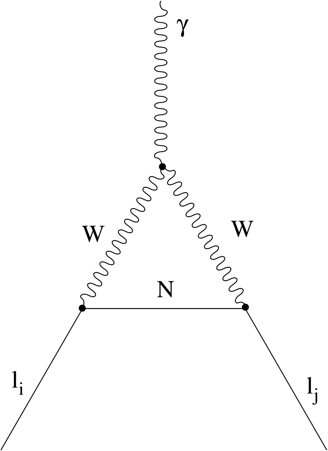
Figure 1: Feynman graphs for $\mu\to e\gamma$ decay in seesaw models.

The resulting decay branching ratio is given by

$$Br(l_{i}\to l_{j}\gamma)=\frac{\alpha^{3}_{W}s_{W}^{2}}{256\pi^{2}}\frac{m_{l_{i}}^{5}}{M_{W}^{4}}\frac{1}{\Gamma_{l_{i}}}|G_{ij}^{W}|^{2}~{},$$ (37)

where we use the explicit analytic form of the loop-functions He:2002pva ,

$$\begin{array}[]{l}G_{ij}^{W}=\sum_{k=1}^{9}K^{*}_{ik}K_{jk}G_{\gamma}^{W}\left(\frac{m^{2}_{N_{k}}}{M_{W}^{2}}\right)~{},\\ G_{\gamma}^{W}(x)=\frac{1}{12(1-x)^{4}}(10-43x+78x^{2}-49x^{3}+18x^{3}\ln{x}+4x^{4}){}\\ \end{array}$$ (38)

and is presented in Fig. 2 for each case. The difference between the two models follows from the different dependence with the lepton number violating parameters that characterize these two low-energy type-I seesaw realizations.

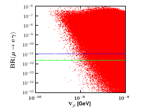
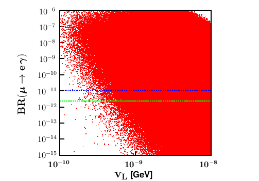
Figure 2: $Br(\mu\to e\gamma)$ versus the lepton number violation scale: $v_{\mu}$ for the inverse seesaw (left panel), and $v_{L}$ for the linear seesaw (right panel). In both cases one assumes normal hierarchy and the parameters are varied as explained in Sec. IV. We also indicate the limits from the MEGA collaboration Ahmed:2001eh (upper line) and the recent limit from MEG :2011ch (lower line).

One sees that the branching rations may easily exceed current limits. This reflects an important feature of low-scale seesaw models, namely, that lepton flavor violation as well as leptonic CP violation proceed even in the limit of massless neutrinos bernabeu:1987gr ; gonzalez-garcia:1991be ; branco:1989bn ; rius:1989gk . Unsuppressed by the smallness of neutrino mass, the expected rates are sizeable. The corresponding radiative LFV decays $\tau\to e\gamma$ and $\tau\to\mu\gamma$ are not as constraining as $\mu\to e\gamma$. Similarly, the fact that the neutral current couplings of charged leptons is flavor diagonal implies that the decay processes $l_{i}\to l_{j}l_{k}l_{r}$ are suppressed by a factor of $\alpha_{QED}$ with respect to the radiative processes, hence less restrictive.

Another very important lepton flavor violating process is mu-e conversion in nuclei, which arises both from short range (non-photonic) as well as long range (photonic) contributions. Explicit calculations deppisch:2005zm indicate that, given the nuclear form factors, one finds that current mu-e conversion sensitivities are effectively lower than those of the $\mu\to e\gamma$ decay. However the upcoming generation of nuclear conversion experiments aims at substantial improvement.

IV Numerical analysis

In order to perform our numerical calculations it is convenient to generalize the Casas-Ibarra parametrization casas:2001sr to the inverse and linear type-I seesaw schemes. For simplicity we will assume real lepton Yukawa couplings and mass entries.

IV.1 Inverse type-I Seesaw

First note that one has always the freedom to go to the basis where the $3\times 3$ gauge-singlet block $M$ is taken diagonal. For real $m_{D}$ matrix elements, we have in total $18$ parameters, nine characterizing $m_{D}$, three characterizing $M$, plus six from the $\mu$ matrix.

The Dirac neutrino mass matrix may be rewritten as

$$m_{D}=V_{1}\,\text{diag}(\sqrt{\tilde{m}_{i}})\,R^{T}\,{(\sqrt{\mu})}^{-1}~{}\text{diag}(M^{T}_{i})$$ (39)

where $V_{1}$ is (approximately) the mixing matrix determined in oscillation experiments Schwetz:2011qt , $\tilde{m}_{i}$ are the three light neutrino masses. On the other hand the arbitrary real orthogonal $3\times 3$ matrix $R$ and the arbitrary $3\times 3$ real matrix $M$ are parameters characterizing the model. This parametrization for the inverse type-I seesaw is similar to that given in Ref. deppisch:2004fa .

In order to further reduce the number of degrees of freedom, we will make the “minimal flavor violation hypothesis”  which consists in assuming that flavor is violated only in the “standard” Dirac Yukawa coupling. Under this simplification the $3\times 3$ matrix $\mu$ must be also diagonal, reducing the parameter count from a total of $18$ down to $15$. These include the three light neutrino masses, and the three neutrino mixing angles contained in $V_{1}$. Next come the nine model-defining parameters, that may be taken as three parameters from the $R$ matrix, three from the $\mu$ matrix, plus three parameters characterizing $M$.

We have performed a scan at $3\sigma$ over the lightest mass and oscillation parameters, the three angles and the three masses in $V_{1}$ and $\tilde{m}_{i}$, respectively. For the scan over oscillation parameters we have used the $3\sigma$ determinations given in Schwetz:2011qt , and for the lightest mass parameter we took the cosmological bound from Fogli:2008 . We parametrize the real orthogonal matrix $R$ as a product of three rotations, marginalizing over the three angles from $0-2\pi$ values.

We have also fixed the upper value of the Dirac mass matrix to $(m_{D})_{ij}<175\,GeV$ to be consistent with perturbativity of the theory. The remaining six free parameters, from $diag\{\mu_{ii}\}$ and $diag\{M_{ii}\}$ matrices, are scanned as a perturbation from the identity matrix in the following way:

$$\begin{split}\mu_{ii}&=v_{\mu}\,\left(1+\varepsilon_{ii}\right)\\ M_{ii}&=v_{M}\,\left(1+\varepsilon^{\prime}_{ii}\right),\end{split}$$ (40)

where $|\varepsilon|\sim 5\times 10^{-1}$. The parameter $v_{M}$ setting the $M$-scale was fixed to $1\,TeV$, while $v_{\mu}$ scale was scanned in the range $(0.1-10)\,eV$. The two scales $v_{\mu,M}$ are consistent with the observed neutrino masses.

IV.2 Linear type-I Seesaw

Similarly, for the linear seesaw case we can parametrize Dirac neutrino mass matrix as follows,

$$m_{D}=V_{1}\text{diag}\{\sqrt{m_{i}}\}\,A^{T}\text{diag}\{\sqrt{m_{i}}\}\,V_{1}^{T}\left(M_{L}^{T}\right)^{-1}\,M^{T},$$ (41)

where $A$ has the following general form:

$$\left(\begin{array}[]{ccc}\frac{1}{2}&a&b\\ -a&\frac{1}{2}&c\\ -b&-c&\frac{1}{2}\end{array}\right),$$ (42)

with $a,b,c$ real numbers. In this case $M_{L}$ and $M\equiv M_{R}$ are general real matrices. One can always go to a basis where one of them is diagonal, for example $M_{L}$, reducing the total number of model parameters to 21.

In order to further reduce the number of degrees of freedom, we make a similar “minimal flavor violation hypothesis” to this scheme too, namely, we choose the $M$ matrix also to be diagonal, reducing from 21 to 15 parameters. The most general Dirac mass matrix is parametrized as in Eq. (41). Hence we have a model with $15$ parameters that may be taken as three parameters from $A$ matrix, three from the $M_{L}$ matrix, three from the matrix $M$, in addition to the three light neutrino masses and three mixing parameters.

As for the inverse type-I seesaw case, we could do the scan over the light neutrino mass and oscillation parameters and the 9 free parameters. The difference in this case respect to the inverse, is the structure of the $A$ matrix in Eq. (42). We scan over the $A$ matrix parameters in the form:

$$A_{ij}\,\,\epsilon\,(0-10^{-2}),$$ (43)

and now we define $M_{Lii}$ in analogy to $M_{ii}$ in Eq. (40) and we vary $v_{L}=(0.01-10)\,eV$.

V Numerical results

Low-scale seesaw schemes lead to sizeable rates for lepton flavor violating processes as well as to non-standard effects in neutrino propagation associated to non-unitary lepton mixing matrix. In this section we will quantify the interplay between these, more precisely, between the branching ratio of Eq. (37) in the low-scale type-I seesaw schemes considered here and the magnitude of the unitarity deviation defined in Eq. (34), taking into account Eqs. (39) and (41) and the requirement of acceptable light neutrino masses. For definiteness we assume leptonic CP conservation so that all lepton Yukawa couplings and mass entries are real.

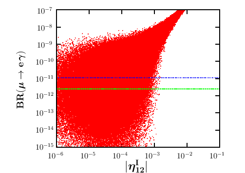
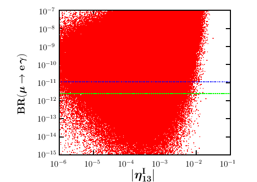
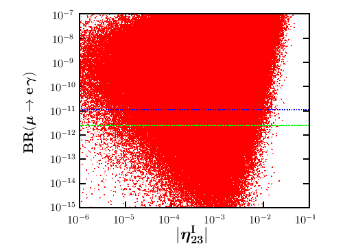
Figure 3: Branching for the process $\mu\to e\gamma$ in type-I inverse seesaw scheme with normal hierarchy (NH). We scan over the light neutrino mass and mixing parameters at 3 $\sigma$, and over the model parameters, fixing $v_{M}$ at 1 $TeV$ and varying the $v_{\mu}$ scale from $1\times 10^{-10}\,GeV$ to $1\times 10^{-8}\,GeV$. We also indicate the limits from the MEGA collaboration (upper line) and the recent limit from MEG (lower line).

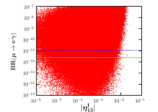
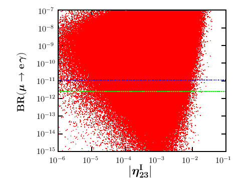
Figure 4: Same as Fig. 3 for the Inverted Hierarchy (IH) case.

We have computed the branching ratio (BR) for the charged lepton flavor violating radiative processes using Eq. (37), accurate to order $O(\epsilon^{3})$ in the neutrino diagonalizing matrix, and displayed the degree of correlation of these observables with the corresponding unitarity violating parameters $|\eta_{ij}|$.

In Fig. 3 and Fig. 4 we show the results for the inverse type-I seesaw scheme with Normal (NH) and Inverted (IH) neutrino mass hierarchy for the process $\mu\to e\gamma$, respectively. The points result from a scan over the light neutrino mass and mixing parameters at 3 $\sigma$, together with the scan over the 9 free model parameters defined above.

In Fig. 5 and Fig. 6 we show the corresponding results for the $\tau\to e\gamma$ branching ratio in the inverse type-I seesaw scheme with Normal Hierarchy (NH) and Inverted Hierarchy (IH), respectively.

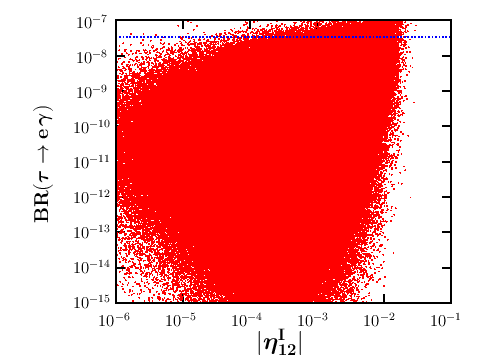
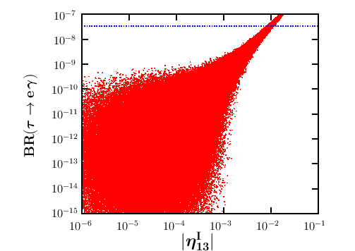
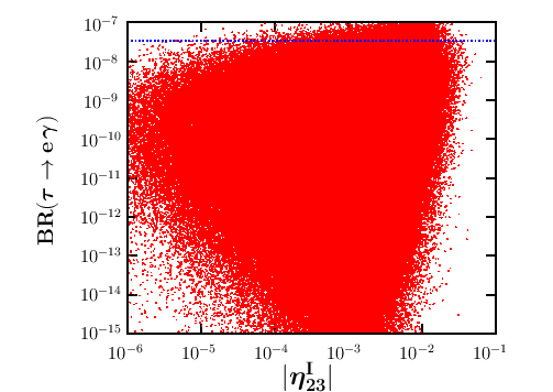
Figure 5: $\tau\to e\gamma$ branching ratio in the inverse type-I seesaw with Normal Hierarchy (NH). The scan is performed as in Fig. 3 and the indicated limit is from the PDG nakamura2010review .

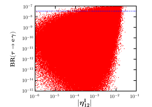
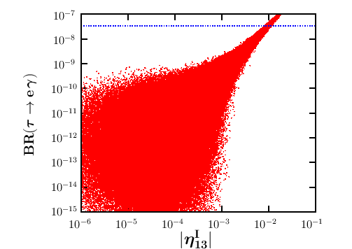
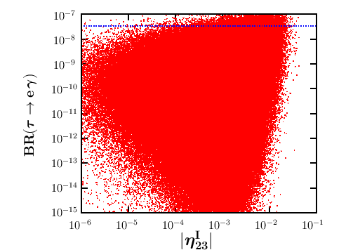
Figure 6: Same as Fig. 5 for Inverted Hierarchy (IH).

In Fig. 7 and Fig. 8 we show the corresponding results for the process $\tau\to\mu\gamma$ within the inverse type-I seesaw, for Normal Hierarchy (NH) and Inverted Hierarchy (IH) neutrino spectra, respectively.

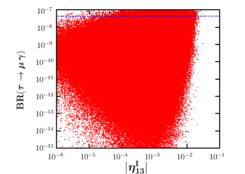
Figure 7: $\tau\to\mu\gamma$ branching ratio in the inverse type-I seesaw with Normal Hierarchy (NH). The scan is performed as in Fig. 3 and the indicated limit is from the PDG nakamura2010review .

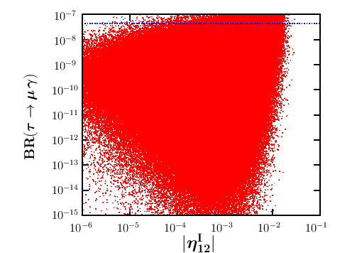
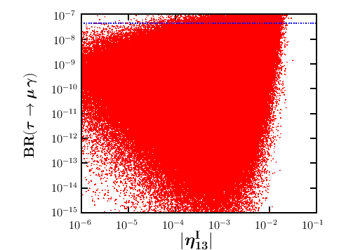
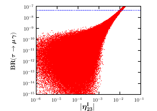
Figure 8: Same as Fig. 7 for Inverted Hierarchy (IH).

Now we turn to the linear type-I seesaw scheme. In Fig. 9 and Fig. 10 we show our results for the branching ratio for the process $\mu\to e\gamma$ in such linear seesaw for Normal Hierarchy (NH) and Inverted Hierarchy (IH), respectively. The points are obtained through a scan over the neutrino oscillation parameters, as well as the free model parameters, as already described.

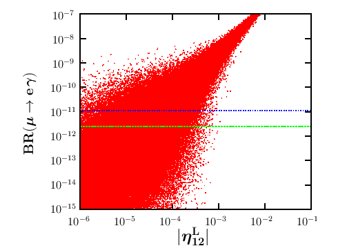
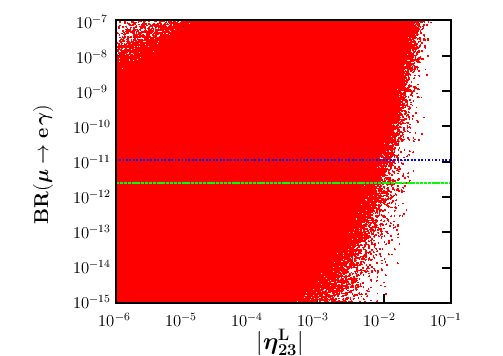
Figure 9: Branching for the process $\mu\to e\gamma$ in type-I linear seesaw with Normal Hierarchy (NH). We scan over the parameters as in Fig. 3. The limits from the MEGA and MEG collaborations are indicated by the upper and lower horizontal lines.

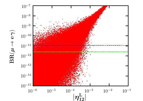
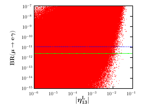
Figure 10: Same as in Fig. 9 for Inverted Hierarchy (IH).

In Fig. 11 and Fig. 12 we show our results for the $\tau\to e\gamma$ branching ratio, for the Normal Hierarchy (NH) and Inverted Hierarchy (IH) case, respectively.

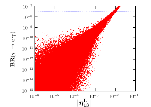
Figure 11: $\tau\to e\gamma$ branching ratio, in Linear type-I seesaw for Normal Hierarchy (NH). Parameters scanned as in Fig. 3 and the indicated limit is from the PDG nakamura2010review .

Figure 12: Same as Fig. 11 for Inverted Hierarchy (IH).

Finally, in Fig. 13 and Fig. 14 we present the corresponding results for the $\tau\to\mu\gamma$ process.

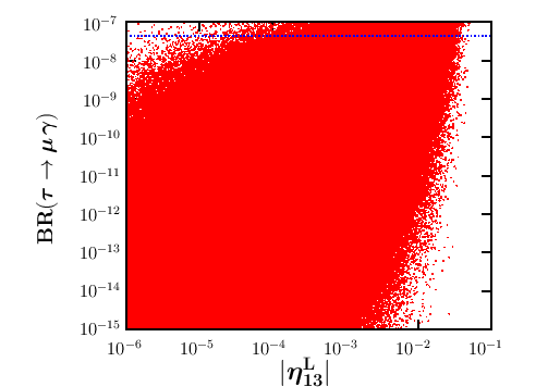
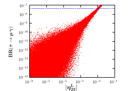
Figure 13: $\tau\to\mu\gamma$ branching ratio, in Linear type-I seesaw for Normal Hierarchy (NH). Parameters scanned as in Fig. 3 and the indicated limit is from the PDG nakamura2010review .

Figure 14: Same as Fig. 11 for Inverted Hierarchy (IH).

These results are summarized in table 1. One sees that the magnitude of non-unitarity effects in the lepton mixing matrix can reach up to percent level is not in conflict with the constraints that follow from lepton flavor violation searches in the laboratory. Given the large - TeV scale - assumed masses of the singlet “right-handed” neutrinos there are no direct search constraints dittmar:1989yg ; Kovalenko:2009td ; Atre:2009rg . The main factor limiting the magnitude of non-unitarity effects then becomes the weak universality constraints. As expected, there is stronger degree of correlation between $\mu\to e\gamma$ and $\eta_{12}$ than other $\eta$’s, or between $\tau\to e\gamma$ and $\eta_{13}$ than others, etc. As a result in these cases one obtains the strongest restriction on unitarity violation.

Process	$\mu\to e\gamma$		$\tau\to e\gamma$		$\tau\to\mu\gamma$
Hierarchy	NH	IH	NH	IH	NH	IH
$|\eta_{12}^{I}|<$	$1.4\times 10^{-3}$	$1.4\times 10^{-3}$	$2.8\times 10^{-2}$	$2.8\times 10^{-2}$	$2.8\times 10^{-2}$	$2.8\times 10^{-2}$
$|\eta_{13}^{I}|<$	$2.0\times 10^{-2}$	$2.1(1.6)\times 10^{-2}$	$1.1\times 10^{-2}$	$1.1\times 10^{-2}$	$3.1\times 10^{-2}$	$3.2\times 10^{-2}$
$|\eta_{23}^{I}|<$	$2.7(2.1)\times 10^{-2}$	$2.5(1.9)\times 10^{-2}$	$6.4\times 10^{-2}$	$4.3\times 10^{-2}$	$1.2\times 10^{-2}$	$1.2\times 10^{-2}$
$|\eta_{12}^{L}|<$	$11.0(9.6)\times 10^{-4}$	$1.5(1.1)\times 10^{-3}$	$5.1\times 10^{-2}$	$5.2\times 10^{-2}$	$5.3\times 10^{-2}$	$5.7\times 10^{-2}$
$|\eta_{13}^{L}|<$	$3.1(2.7)\times 10^{-2}$	$3.3\times 10^{-2}$	$1.1\times 10^{-2}$	$1.0\times 10^{-2}$	$4.8\times 10^{-2}$	$4.8\times 10^{-2}$
$|\eta_{23}^{L}|<$	$2.8(2.2)\times 10^{-2}$	$3.0\times 10^{-2}$	$5.5\times 10^{-2}$	$5.4\times 10^{-2}$	$1.2\times 10^{-2}$	$1.2\times 10^{-2}$

Table 1: Limits on unitarity violation parameters from lepton flavor violation searches. The numbers given in parenthesis correspond to the improvement obtained with the recent MEG limit on $\mu\to e\gamma$. Other entries in the table are unchanged. These limits express the correlation between lepton non-unitarity and LFV that holds in low-scale seesaw schemes under a “minimal flavor violation hypothesis” defined in the text.

Before closing let us comment on the robustness or our results with respect to the assumptions made in Sec. IV. Insofar as the regions obtained in Figs. (3)-(14) are concerned, we can state that they remain “allowed” once one departs from our simplifying assumptions. As expected however, we have verified that the regions obtained away from the simplifying assumptions may allow for somewhat larger values of the lepton-flavor-violating parameters $\eta$ affecting neutrino propagation. However, on account of weak universality constraints, we prefer to stick to the more conservative values we have presented in Table 1.

VI Conclusions

The physics responsible for neutrino masses could lie at the TeV scale. In this case it is very unlikely that neutrino masses are not accompanied by non-standard neutrino interactions that could reveal novel features in neutrino propagation. Similarly, lepton flavor violation should also take place in processes involving the charged leptons.

Within low-scale seesaw mechanisms, such as the inverse and linear type-I seesaw, we have found that non-unitarity in the lepton mixing matrix up to the percent level in some cases, is consistent with the constraints that follow from lepton flavor violation searches in the laboratory. This conclusion holds even within the simple “minimal flavor violation” assumptions we have made. As a result the upcoming long baseline neutrino experiments bandyopadhyay:2007kx do provide an important window of opportunity to perform complementary tests of lepton flavor violation in neutrino propagation and to probe the mass scale characterizing the seesaw mechanism.

VII Acknowledgments

We thank M. Hirsch for useful discussions. This work was supported by the Spanish MICINN under grants FPA2008-00319/FPA and MULTIDARK CSD2009-00064, by Prometeo/2009/091 (Generalitat valenciana), by the EU Network grant UNILHC PITN-GA-2009-237920. S. M. is supported by a Juan de la Cierva contract, M. T. acknowledges financial support from CSIC under the JAE-Doc programme.

References

- (1) S. Weinberg, Phys. Rev. D22, 1694 (1980).
- (2) T. Schwetz, M. Tortola, and J. W. F. Valle, New J. Phys. 13, 063004 (2011), latest T2K/MINOS results in addendum in arXiv:1108.1376 [hep-ph] (to be published).
- (3) R. Mohapatra, Talk at Neutrino 2010 Conference, Athens.
- (4) J. W. F. Valle, J. Phys. Conf. Ser. 53, 473 (2006), Review lectures at Corfu, hep-ph/0608101.
- (5) J. Schechter and J. W. F. Valle, Phys. Rev. D22, 2227 (1980).
- (6) J. Schechter and J. W. F. Valle, Phys. Rev. D25, 774 (1982).
-
(7)
R. N. Mohapatra and J. W. F. Valle,
Phys. Rev. D34, 1642 (1986);
M. C. Gonzalez-Garcia and J. W. F. Valle, B216, 360 (1989). - (8) M. Malinsky, J. C. Romao, and J. W. F. Valle, Phys. Rev. Lett. 95, 161801 (2005).
- (9) J. Bernabeu et al., Phys. Lett. B187, 303 (1987).
- (10) M. C. Gonzalez-Garcia and J. W. F. Valle, Mod. Phys. Lett. A7, 477 (1992).
- (11) G. C. Branco, M. N. Rebelo, and J. W. F. Valle, Phys. Lett. B225, 385 (1989).
- (12) N. Rius and J. W. F. Valle, Phys. Lett. B246, 249 (1990).
- (13) S. Antusch, J. P. Baumann, and E. Fernandez-Martinez, Nucl. Phys. B810, 369 (2009), 0807.1003.
- (14) M. Malinsky, T. Ohlsson, and H. Zhang, Phys. Rev. D79, 073009 (2009), 0903.1961.
- (15) P. Dev and R. Mohapatra, Phys.Rev. D81, 013001 (2010), 0910.3924.
- (16) J. W. F. Valle, Phys. Lett. B199, 432 (1987).
-
(17)
H. Nunokawa et al.,
Phys. Rev. D54, 4356 (1996);
A. Esteban-Pretel, R. Tomas, and J. W. F. Valle, Phys. Rev. D76, 053001 (2007). -
(18)
O. G. Miranda, M. A. Tortola, J. W. F. Valle,
JHEP 0610, 008 (2006);
N. Fornengo, M. Maltoni, R. Tomas, J. W. F. Valle, Phys. Rev. D65, 013010 (2002). - (19) B. W. Lee and R. E. Shrock, Phys. Rev. D16, 1444 (1977).
- (20) K. Nakamura et al., Journal of Physics G: Nuclear and Particle Physics 37, 075021 (2010).
- (21) MEG collaboration, J. Adam et al., (2011), 1107.5547.
- (22) MEGA collaboration, M. Ahmed et al., Phys. Rev. D65, 112002 (2002), hep-ex/0111030.
-
(23)
D. Ibanez, S. Morisi, and J. W. F. Valle,
Phys. Rev. D80, 053015 (2009), [arXiv:0907.3109 [hep-ph]];
J. F. Kamenik, M. Nemevsek, JHEP 0911, 023 (2009), [arXiv:0908.3451 [hep-ph]]. - (24) ISS Physics Working Group, A. Bandyopadhyay et al., Rep. Prog. Phys. 72, 106201 (2009).
- (25) G. t’Hooft, Lectures at Cargese Summer Inst. 1979, p.345-367, Ed. by E. Farhi et al. (World Scientific, Singapore)
- (26) D. Wyler and L. Wolfenstein, Nucl. Phys. B218, 205 (1983).
- (27) E. Akhmedov et al., Phys. Rev. D53, 2752 (1996), hep-ph/9509255.
- (28) S. M. Barr and I. Dorsner, Phys. Lett. B632, 527 (2006), hep-ph/0507067.
- (29) F. Bazzocchi et. al., Phys.Rev. D81, 051701 (2010), 0907.1262.
- (30) E. Akhmedov et al., Phys. Lett. B368, 270 (1996), hep-ph/9507275.
- (31) M. Hirsch, S. Morisi, and J. Valle, Phys. Lett. B 679, 454 (2009).
- (32) H. Hettmansperger, M. Lindner, and W. Rodejohann, arXiv:1102.3432v1 [hep-ph].
- (33) S. L. Glashow, J. Iliopoulos, and L. Maiani, Phys. Rev. D2, 1285 (1970).
- (34) A. Ilakovac and A. Pilaftsis, Nucl. Phys. B437, 491 (1995), hep-ph/9403398.
- (35) F. Deppisch and J. W. F. Valle, Phys. Rev. D72, 036001 (2005), hep-ph/0406040.
- (36) B. He, T. Cheng, and L.-F. Li, Phys.Lett. B553, 277 (2003), hep-ph/0209175.
- (37) L. Lavoura, Eur. Phys. J. C29, 191 (2003), hep-ph/0302221.
- (38) F. Deppisch, T. S. Kosmas, and J. W. F. Valle, Nucl. Phys. B752, 80 (2006), hep-ph/0512360.
- (39) J. A. Casas and A. Ibarra, Nucl. Phys. B618, 171 (2001), hep-ph/0103065.
- (40) G. D’Ambrosio, G. Giudice, G. Isidori, and A. Strumia, Nucl.Phys. B645, 155 (2002), hep-ph/0207036.
- (41) V. Cirigliano, B. Grinstein, G. Isidori, and M. B. Wise, Nucl.Phys. B728, 121 (2005), hep-ph/0507001.
- (42) R. Alonso, G. Isidori, L. Merlo, L. A. Munoz, and E. Nardi, JHEP 1106, 037 (2011), 1103.5461.
- (43) G. L. Fogli, E. Lisi, A. Marrone, A. Melchiorri, A. Palazzo, A. M. Rotunno, P. Serra, J. Silk, and A. Slosar, Phys. Rev. D 78, 033010 (2008).
- (44) M. Dittmar, A. Santamaria, M. C. Gonzalez-Garcia, and J. W. F. Valle, Nucl. Phys. B332, 1 (1990).
- (45) S. Kovalenko, Z. Lu, and I. Schmidt, Phys.Rev. D80, 073014 (2009), 0907.2533.
- (46) A. Atre, T. Han, S. Pascoli, and B. Zhang, JHEP 0905, 030 (2009), 0901.3589.