Metastable states of hydrogen: their geometric phases and flux densities

Abstract

We discuss the geometric phases and flux densities for the metastable states of hydrogen with principal quantum number $n=2$ being subjected to adiabatically varying external electric and magnetic fields. Convenient representations of the flux densities as complex integrals are derived. Both, parity conserving (PC) and parity violating (PV) flux densities and phases are identified. General expressions for the flux densities following from rotational invariance are derived. Specific cases of external fields are discussed. In a pure magnetic field the phases are given by the geometry of the path in magnetic field space. But for electric fields in presence of a constant magnetic field and for electric plus magnetic fields the geometric phases carry information on the atomic parameters, in particular, on the PV atomic interaction. We show that for our metastable states also the decay rates can be influenced by the geometric phases and we give a concrete example for this effect. Finally we emphasise that the general relations derived here for geometric phases and flux densities are also valid for other atomic systems having stable or metastable states, for instance, for He with $n=2$. Thus, a measurement of geometric phases may give important experimental information on the mass matrix and the electric and magnetic dipole matrices for such systems. This could be used as a check of corresponding theoretical calculations of wave functions and matrix elements.
HD–THEP–11–05

1 Introduction

In this paper we study properties of geometric phases and geometric flux densities for metastable hydrogen atoms in external electric and magnetic fields. Geometric phases in quantum mechanics were introduced in Ber84 and have been studied extensively since then; see for instance Bar83 ; ShWi89 ; Nak90 and references therein. For a discussion of geometric phases for systems described by a non-hermitian Hamiltonian see Garrison1988177 ; Massar1996 ; KeKoMo2003 ; Berry2004 ; Heiss2004 ; NesCru2008 and references therein. In our group the adiabatic theorem and geometric phases for metastable states were studied in BeGaNa07_I ; BeGaNa07_II . Both, parity conserving (PC), and parity violating (PV) geometric phases were identified. One aim is to apply the theory developed in this way to the measurement of parity violation in light atoms like hydrogen with the longitudinal spin echo technique; see ABSE95 ; BeGaMaNaTr08_I ; DeKGaNaTr11 . But, clearly, a measurement of geometric phases is very interesting by itself since these phases represent a deep quantum-mechanical phenomenon. For metastable states these phases are complex and, therefore, geometry also influences the decay rates of these states, as we shall demonstrate explicitly below.

In the present paper we are primarily interested in the structure of PC and PV geometric phases and flux densities, that is, what one can say on general grounds about their dependences on the external electric and magnetic fields. Since a measurement of PV geometric phases is one possibility to study atomic parity violation (APV) we briefly refer to recent work discussing the present status of this field. Standard reviews of APV can be found in Khrip91 ; Bou97 . A very recent survey of the past, present, and prospects of APV is given in Bou2011 . Experimental results for the heavy atoms Cs Bouchiat1982358 ; Wood1997 ; BeWi99 , Bi Macpherson1991 , Tl Edwards1995 ; Vet95 , Pb Mee93 , and Yb Budker2009 have been published. See also the review in PDG10 . A large effort is being undertaken to measure APV in Ra⁺ Wansbeek2008 ; Versolato2011 , and plans for the future FAIR facility at GSI, Darmstadt, include a program of APV studies for highly charged ions PhysRevA.40.7362 ; PhysRevA.63.054105 ; Shabaev10 ; PhysRevA.81.062503 ; Surzhykov11 . The situation for APV in the lightest atoms, H and D, is nicely summarised in DuHo07 ; DuHo11 . In these latter papers it is also stressed that from the theory point of view H and D are the ideal candidates to study APV.

Our paper is organised as follows. In Section 2 we introduce the atomic systems which we want to study. In Section 3 we define the geometric phases and flux densities and derive useful representations for them in terms of complex integrals. Section 4 is devoted to a study of the structure of these phases and flux densities following from rotational invariance. In Section 5 we discuss specific cases. Section 6 presents our conclusions. In Appendix A we explain the notations used throughout our work and provide many useful formulae as well as essential numerical quantities. In addition, we give the non-zero parts of the mass matrix for the $n=2$ states of hydrogen. In the Appendices B, C and D we present detailed proofs for the relations derived in Sections 3, 4, and 5, respectively. In Appendix E (online only) we give explicit formulae for various matrices used in our paper. If not stated otherwise we use natural units with $\hbar=c=1$.

2 Metastable hydrogen states in external fields

Figure 1: Energy levels of the hydrogen states with principal quantum number $n=2$ in vacuum. The numerical values of the fine structure splitting $\Delta$, the Lamb shift $L$ and the ground state hyperfine splitting energy $\mathcal{A}$ are given in Table 1 of Appendix A.

We are interested in the states of hydrogen with principal quantum number $n=2$. Their energy levels in vacuum are shown in Figure 1. The lifetimes $\tau$ of the 2S and 2P states of hydrogen in vacuum are $\tau_{S}=\Gamma_{S}^{-1}=0.1216\,$s and $\tau_{P}=\Gamma_{P}^{-1}=1.596\times 10^{-9}\,$s, respectively; see Sap04 ; LaShSo05 . Here $\Gamma_{S,P}$ are the decay rates. We have 16 states with $n=2$ for which we use a numbering scheme $\alpha=1,\dots,16$ as explained in Appendix A, Table 2.

In this paper we shall consider $n=2$ hydrogen atoms at rest subjected to slowly varying electric and magnetic fields. In vacuum the 2S states of hydrogen are metastable and decay by two-photon emission to the ground state. The 2P states decay to the ground state by one-photon emission. Energetically allowed radiative decays from one $n=2$ state to another one are completely negligible. This remains true when we consider the $n=2$ states in an external, slowly varying, electromagnetic field in the adiabatic limit. There, by definition, the variation of the external fields has to be slow enough such that no transitions between the $n=2$ levels are induced. In this situation we can apply the standard Wigner-Weisskopf method WeWi30 ; WeWi30b . The derivation of this method and its limitations are discussed in many textbooks and articles, see for instance MaWo95 ; BaRa97 ; Knight197299 ; Wang1974323 ; BeNa83 ; Nac90 ; BoBrNa95 . A derivation starting from quantum field theory can be found in PhysRev.121.350 ; RG1963239 . Let us note that for more complex situations than discussed in the present paper, for instance if radiative transitions are induced between the $n=2$ states by an external field, we would have to use other methods, master equations, the optical Bloch equation etc.; see BaRa97 .

Thus, for the situations we are considering the basic theoretical tool is the effective Schrödinger equation describing the evolution of the undecayed states with state vector $|t)$ at time $t$, in the Wigner-Weisskopf approximation,

$$\mathrm{i}\frac{\partial}{\partial t}|t)=\underline{\mathscr{M}}(\bm{\mathcal{E}}(t),\bm{\mathcal{B}}(t))|t)\ .$$ (1)

Here

$$\underline{\mathscr{M}}(\bm{\mathcal{E}}(t),\bm{\mathcal{B}}(t))=\underline{\mathscr{\tilde{M}}}_{0}-\underline{\bm{D}}\cdot\bm{\mathcal{E}}(t)-\underline{\bm{\mu}}\cdot\bm{\mathcal{B}}(t)$$ (2)

with $\underline{\mathscr{\tilde{M}}}_{0}$ the mass matrix for the $n=2$ states in vacuum, $\underline{\bm{D}}$ and $\underline{\bm{\mu}}$ the electric and magnetic dipole operators, respectively, in the $n=2$ subspace, and $\bm{\mathcal{E}}$ and $\bm{\mathcal{B}}$ the electric and magnetic fields. We are interested in parity conserving (PC) and parity violating (PV) geometric phases. The mass matrix $\underline{\mathscr{\tilde{M}}}_{0}$ will therefore be split into the PC part $\underline{\mathscr{M}}_{0}$ and the PV part $\delta\,\underline{\mathscr{M}}_{\mathrm{PV}}$,

$$\underline{\mathscr{\tilde{M}}}_{0}=\underline{\mathscr{M}}_{0}+\delta\,\underline{\mathscr{M}}_{\mathrm{PV}}\ .$$ (3)

In the standard model of particle physics (SM) $\delta\,\underline{\mathscr{M}}_{\mathrm{PV}}$ is determined by Z-boson exchange between the electrons of the hull and the quarks in the nucleus. Here, as in BeGaNa07_II , we split off a (very small) numerical factor $\delta$ from the PV part of the mass matrix characterising the intrinsic strength of the PV terms. In Appendix A we give explicitly $\delta$. The matrices $\underline{\mathscr{\tilde{M}}}_{0}$, $\underline{\bm{D}}$ and $\underline{\bm{\mu}}$ are discussed further in Appendix A, and their explicit forms used for numerical purposes are given in Appendix E; see Tables 3, 4, and 5.

In the presence of electric fields the metastable 2S states will get a 2P admixture making them decay faster, see Figure 1 of BeGaNa07_II . We are interested in the situation where the lifetime of the metastable states is still at least a factor of 5 larger than that of the other states. As shown in (27) of BeGaNa07_II this limits us to electric fields

$$|\bm{\mathcal{E}}|\lesssim 250\,\mbox{V/cm}\ .$$ (4)

In BeGaNa07_I ; BeGaNa07_II the adiabatic theorem and geometric phases for metastable states were studied and in the present work we shall apply and extend the results obtained there. The mass matrix $\underline{\mathscr{M}}$ in (1) depends on the slowly varying parameters $\bm{\mathcal{E}}$ and $\bm{\mathcal{B}}$. Thus, we have a six-dimensional parameter space. Geometric phases are connected with the trajectories followed by the field strengths as function of time in this space.

In the following we shall, for general discussions, denote $\bm{\mathcal{E}}$ and $\bm{\mathcal{B}}$ collectively as parameters $K$,

$$\left(\begin{array}[]{c}\bm{\mathcal{E}}\\ \bm{\mathcal{B}}\end{array}\right)=\left(\begin{array}[]{c}K_{1}\\ K_{2}\\ K_{3}\\ K_{4}\\ K_{5}\\ K_{6}\end{array}\right)\equiv K\ .$$ (13)

Indices $i,j\in\{1,2,3\}$ will be normal space indices, for instance $\mathcal{E}_{i}$, $\mathcal{B}_{i}$ etc., or refer to any three particular components of $K$. Indices $a$, $b$ shall refer to the components $K_{a}$, $a\in\{1,\dots,6\}$. The mass matrix (2) shall be considered as function of the six parameters $K=K_{a}$

$$\underline{\mathscr{M}}(\bm{\mathcal{E}},\bm{\mathcal{B}})\equiv\underline{\mathscr{M}}(K)\ .$$ (14)

We shall assume that we work in a region of parameter space ($K$ space) where $\underline{\mathscr{M}}(K)$ can be diagonalised. There are then 16 linearly independent right and left eigenvectors of $\underline{\mathscr{M}}(K)$,

$$\underline{\mathscr{M}}(K)|\alpha,K) =E_{\alpha}(K)|\alpha,K)\ ,$$

$$(\widetilde{\alpha,K}|\underline{\mathscr{M}}(K) =(\widetilde{\alpha,K}|E_{\alpha}(K)\ ,$$

$$(\alpha =1,\dots,16)\ .$$ (15)

These eigenvectors satisfy

$$(\widetilde{\alpha,K}|\beta,K)=\delta_{\alpha\beta}\ .$$ (16)

As normalisation condition we choose

$$(\alpha,K|\alpha,K)=1$$

$$\mbox{(no summation over $\alpha$)}\ .$$ (17)

The complex energies are

$$E_{\alpha}(K)=E_{\alpha R}(K)-\frac{\mathrm{i}}{2}\Gamma_{\alpha}(K)$$ (18)

with $E_{\alpha R}$ the real part of the energy and $\Gamma_{\alpha}(K)=$ $\big{(}\tau_{\alpha}(K)\big{)}^{-1}$ the decay rate, that is, the inverse lifetime of the state $|\alpha,K)$. In the following we shall suppose

$$|E_{\alpha}(K)-E_{\beta}(K)|\geq c>0$$ (19)

for all $\alpha\not=\beta$ where $c$ is a constant. Exceptions where (19) is not required to hold will be clearly indicated.

Below we shall make extensive use of the quasi projectors defined as

$$\mathbbm{P}_{\alpha}(K)=|\alpha,K)(\widetilde{\alpha,K}|\ .$$ (20)

These satisfy

$$\mathbbm{P}_{\alpha}(K)\mathbbm{P}_{\beta}(K) =\left\{\begin{array}[]{cl}\mathbbm{P}_{\alpha}(K)&\mbox{for }\alpha=\beta\ ,\\ 0&\mbox{for }\alpha\not=\beta\ ,\end{array}\right.$$ (23)

$$\sum_{\alpha}\mathbbm{P}_{\alpha}(K) =\mathbbm{1}\ ,$$ (24)

but, in general, the $\mathbbm{P}_{\alpha}(K)$ are non-hermitian matrices. Furthermore, we shall need the resolvent $\big{(}\zeta-\underline{\mathscr{M}}(K)\big{)}^{-1}$ where $\zeta$ is arbitrary complex. With the help of the quasi projectors we get

$$\big{(}\zeta-\underline{\mathscr{M}}(K)\big{)}^{-n} =\sum_{\alpha}\big{(}\zeta-E_{\alpha}(K)\big{)}^{-n}\mathbbm{P}_{\alpha}(K)\ ,$$

$$(n =0,1,2,\dots)\ .$$ (25)

Now we come back to the effective Schrödinger equation (1) which reads, replacing $(\bm{\mathcal{E}},\bm{\mathcal{B}})$ by $K$,

$$\mathrm{i}\frac{\partial}{\partial t}|t)=\underline{\mathscr{M}}(K(t))|t)\ .$$ (26)

The state vector is expanded as

$$|t)=\sum_{\alpha=1}^{16}\psi_{\alpha}(t)|\alpha,K(t))\ .$$ (27)

We always suppose slow enough variation of the parameter vector $K(t)$. As shown in Section 3 of BeGaNa07_II we get then the solution of (26) for the metastable states as follows.

We consider an initial metastable state at time $t=0$

$$|t=0)=\sum_{\alpha\in I}\psi_{\alpha}(0)|\alpha,K(0))$$ (28)

where $\alpha$ only runs over the index set of the metastable states,

$$I=\{9,10,11,12\}\ ,$$ (29)

in our numbering scheme. Then we have, for $t\geq 0$,

$$|t)=\sum_{\alpha\in I}\psi_{\alpha}(t)|\alpha,K(t))$$ (30)

where

$$\psi_{\alpha}(t) =\exp\big{[}-\mathrm{i}\varphi_{\alpha}(t)+\mathrm{i}\gamma_{\alpha}(t)\big{]}\psi_{\alpha}(0)\ ,$$ (31)

$$\varphi_{\alpha}(t) =\int_{0}^{t}\mathrm{d}t^{\prime}\,E_{\alpha}(K(t^{\prime}))\ ,$$ (32)

$$\gamma_{\alpha}(t) =\int_{0}^{t}\mathrm{d}t^{\prime}(\widetilde{\alpha,K(t^{\prime})}|\mathrm{i}\frac{\partial}{\partial t^{\prime}}|\alpha,K(t^{\prime}))\ .$$ (33)

The quantities $\varphi_{\alpha}(t)$ and $\gamma_{\alpha}(t)$ are the familiar dynamic and geometric phases, respectively. For metastable states both will in general have real and imaginary parts.

Here and in the following the labels $\alpha=9,10,11$, and $12$ correspond to the states $|\alpha,K)\equiv|2\hat{S}_{1/2},F,F_{3},\bm{\mathcal{E}},\bm{\mathcal{B}})$. These originate from the states $|2S_{1/2},F,F_{3})$ with $(F,F_{3})=(1,1)$, $(1,0)$, $(1,-1)$, and $(0,0)$, respectively, through the mixing with the 2P states according to the $\mathrm{PV}$, the $\bm{\mathcal{E}}$, and $\bm{\mathcal{B}}$ terms in the mass matrix (2). This numbering has to be carefully defined, see Appendix A, since we have to follow the states in their adiabatic motion along trajectories in parameter space. As explained in Appendix A $(F,F_{3})$ are then only labels of the states, no longer the total angular momentum quantum numbers. Thus, in order to avoid confusion, we shall stick to the labels $\alpha$ for our states in the following.

Below we shall study in detail the geometric phases for metastable states for the case that $K(t)$ makes a closed loop in parameter space.

3 Geometric phases and flux densities

In this section we shall discuss general relations and properties for geometric phases and the corresponding flux densities defined below. These relations hold for any system with time evolution described by an effective Schrödinger equation

$$\mathrm{i}\frac{\partial}{\partial t}|t)=\underline{\mathscr{M}}(K(t))|t)\ ,$$ (34)

with $N\times N$ matrices $\underline{\mathscr{M}}(K)$, and having metastable states. The parameter vector $K$ can have any number of components and the dependence of $\underline{\mathscr{M}}$ on $K$ need not be linear as for $\underline{\mathscr{M}}(\bm{\mathcal{E}},\bm{\mathcal{B}})=\underline{\mathscr{M}}(K)$ in Section 2.

We consider now the system over a time interval
$0\leq t\leq T$ where the parameter vector $K(t)$ runs over a closed curve $\mathcal{C}$

$$\mathcal{C}\,:\,t\rightarrow K(t),\;t\in[0,T],\;K(T)=K(0)\ .$$ (35)

The geometric phases (33) acquired by the metastable states are then

$$\gamma_{\alpha}(\mathcal{C})\equiv\gamma_{\alpha}(T) =\int_{0}^{T}\mathrm{d}t^{\prime}(\widetilde{\alpha,K(t^{\prime})}|\mathrm{i}\frac{\partial}{\partial t^{\prime}}|\alpha,K(t^{\prime}))$$

$$=\int_{\mathcal{C}}(\widetilde{\alpha,K}|\mathrm{i}\,\mathrm{d}|\alpha,K)\ ,$$ (36)

$\alpha\in I$, where $I$ is the index set of the metastable states. For our concrete hydrogen case $I$ is given in (29). Here and in the following we use the exterior derivative calculus; see for instance Fla63 . Let $\mathcal{F}$ be a surface with boundary $\mathcal{C}$,

$$\partial\mathcal{F}=\mathcal{C}\ ,$$ (37)

and suppose that $\underline{\mathscr{M}}(K)$ can be diagonalised for all $K\in\mathcal{F}$, and (19) holds for the eigenvalues. We get then

$$\gamma_{\alpha}(\mathcal{C}) =\mathrm{i}\int_{\partial\mathcal{F}}(\widetilde{\alpha,K}|\mathrm{d}|\alpha,K)$$

$$=\mathrm{i}\int_{\mathcal{F}}\mathrm{d}(\widetilde{\alpha,K}|\mathrm{d}|\alpha,K)$$

$$=\int_{\mathcal{F}}Y_{\alpha,ab}(K)\,\mathrm{d}K_{a}\wedge\mathrm{d}K_{b}\ .$$ (38)

Here we define the geometric flux densities $Y_{\alpha,ab}(K)$, the analogues for the metastable states of the quantities $\bm{V}$ of Ber84 , by

$$Y_{\alpha,ab}\,\mathrm{d}K_{a}\wedge\mathrm{d}K_{b} =\mathrm{i}\,\mathrm{d}(\widetilde{\alpha,K}|\mathrm{d}|\alpha,K)\ ,$$

$$Y_{\alpha,ab}(K)+Y_{\alpha,ba}(K) =0\ .$$ (39)

From (3) we get easily

$$Y_{\alpha,ab}(K)\,\mathrm{d}K_{a}\wedge\mathrm{d}K_{b} =+\mathrm{i}\big{(}\mathrm{d}(\widetilde{\alpha,K}|\big{)}\wedge\big{(}\mathrm{d}|\alpha,K)\big{)}$$

$$=-\mathrm{i}\sum_{\beta\not=\alpha}(\widetilde{\alpha,K}|\mathrm{d}|\beta,K)\wedge(\widetilde{\beta,K}|\mathrm{d}|\alpha,K)\ .$$ (40)

Here we use

$$\big{(}\mathrm{d}(\widetilde{\alpha,K}|\big{)}|\beta,K)+(\widetilde{\alpha,K}|\mathrm{d}|\beta,K)=0$$ (41)

which follows from (16). Note that in (3) $\alpha$ is the index of a metastable state, $\alpha\in I$, but in the sum over $\beta$ all states with $\beta\not=\alpha$ have to be included.

As a further relation following directly from (3) we get the generalised divergence condition

$$\mathrm{d}\big{(}Y_{\alpha,ab}(K)\,\mathrm{d}K_{a}\wedge\mathrm{d}K_{b}\big{)}=\mathrm{i}\,\mathrm{dd}(\widetilde{\alpha,K}|\mathrm{d}|\alpha,K)=0$$ (42)

which implies

$$\frac{\partial}{\partial K_{a}}Y_{\alpha,bc}(K)+\frac{\partial}{\partial K_{b}}Y_{\alpha,ca}(K)+\frac{\partial}{\partial K_{c}}Y_{\alpha,ab}(K)=0\ .$$ (43)

Let us now derive further representations and properties for the geometric flux densities. From (15) and (16) we get for $\beta\not=\gamma$

$$(\widetilde{\beta,K}|\underline{\mathscr{M}}(K)|\gamma,K)=0\ .$$ (44)

Taking the exterior derivative in (44) gives

$$[E_{\beta}(K)-E_{\gamma}(K)](\widetilde{\beta,K}|\mathrm{d}|\gamma,K)$$

$$\qquad\qquad+(\widetilde{\beta,K}|\big{(}\mathrm{d}\underline{\mathscr{M}}(K)\big{)}|\gamma,K)=0\ .$$ (45)

Since we suppose (19) to hold for all $K\in\mathcal{F}$ we get for $\beta\not=\gamma$

$$(\widetilde{\beta,K}|\mathrm{d}|\gamma,K)=-\frac{(\widetilde{\beta,K}|\big{(}\mathrm{d}\underline{\mathscr{M}}(K)\big{)}|\gamma,K)}{E_{\beta}(K)-E_{\gamma}(K)}\ .$$ (46)

Inserting this in (3) gives

$$Y_{\alpha,ab}(K) =\frac{\mathrm{i}}{2}\sum_{\beta\not=\alpha}[E_{\alpha}(K)-E_{\beta}(K)]^{-2}$$

$$\times(\widetilde{\alpha,K}|\frac{\partial\underline{\mathscr{M}}(K)}{\partial K_{a}}|\beta,K)(\widetilde{\beta,K}|\frac{\partial\underline{\mathscr{M}}(K)}{\partial K_{b}}|\alpha,K)$$

$$-(a\leftrightarrow b)$$

$$=\frac{\mathrm{i}}{2}\sum_{\beta\not=\alpha}[E_{\alpha}(K)-E_{\beta}(K)]^{-2}$$

$$\times\mathrm{Tr}\Big{[}\mathbbm{P}_{\alpha}(K)\frac{\partial\underline{\mathscr{M}}(K)}{\partial K_{a}}\mathbbm{P}_{\beta}(K)\frac{\partial\underline{\mathscr{M}}(K)}{\partial K_{b}}$$

$$\hskip 120.00018pt-(a\leftrightarrow b)\Big{]}$$ (47)

where we use the quasi projectors (20).

Figure 2: The complex $\zeta$ plane with the (schematic) location of the energy eigenvalues $E_{\alpha}(K)$ and $E_{\beta}(K)$ with $\beta\not=\alpha$. The curve $S_{\alpha}$ encircles only $E_{\alpha}(K)$.

We shall now derive an integral representation for $Y_{\alpha,ab}(K)$. Consider the complex $\zeta$ plane, see Figure 2, where we mark schematically the position of the energy eigenvalues $E_{\alpha}(K)$ and $E_{\beta}(K)$, $\beta\not=\alpha$. Since we suppose (19) to hold we can choose a closed curve $S_{\alpha}$ which encircles only $E_{\alpha}(K)$ but where all $E_{\beta}(K)$ with $\beta\not=\alpha$ are outside. The geometric flux densities (3), (3) are then given as a complex integral

$$Y_{\alpha,ab}(K)=\frac{\mathrm{i}}{2}\frac{1}{2\pi\mathrm{i}}\oint_{S_{\alpha}}\mathrm{d}\zeta\,\mathrm{Tr}\Big{[}\frac{1}{(\zeta-\underline{\mathscr{M}}(K))}\frac{\partial\underline{\mathscr{M}}(K)}{\partial K_{a}}$$

$$\hfill\times\frac{1}{(\zeta-\underline{\mathscr{M}}(K))^{2}}\frac{\partial\underline{\mathscr{M}}(K)}{\partial K_{b}}\Big{]}\ .$$ (48)

The proof of (3) is given in Appendix B. From (3) we get convenient relations for the derivatives of $Y_{\alpha,ab}(K)$, see Appendix B,

$$\frac{\partial}{\partial K_{a}} Y_{\alpha,bc}(K)=\frac{\mathrm{i}}{2}\frac{1}{2\pi\mathrm{i}}\oint_{S_{\alpha}}\mathrm{d}\zeta\Big{\{}$$

$$\mathrm{Tr}\Big{[}\frac{1}{(\zeta-\underline{\mathscr{M}}(K))}\frac{\partial^{2}\underline{\mathscr{M}}(K)}{\partial K_{a}\partial K_{b}}\frac{1}{(\zeta-\underline{\mathscr{M}}(K))^{2}}\frac{\partial\underline{\mathscr{M}}(K)}{\partial K_{c}}\Big{]}$$

$$+ \mathrm{Tr}\Big{[}\frac{1}{(\zeta-\underline{\mathscr{M}}(K))}\frac{\partial\underline{\mathscr{M}}(K)}{\partial K_{a}}\frac{1}{(\zeta-\underline{\mathscr{M}}(K))}\frac{\partial\underline{\mathscr{M}}(K)}{\partial K_{b}}$$

$$\qquad\qquad\times\frac{1}{(\zeta-\underline{\mathscr{M}}(K))^{2}}\frac{\partial\underline{\mathscr{M}}(K)}{\partial K_{c}}\Big{]}\Big{\}}-(b\leftrightarrow c)\ ,$$ (49)

which can also be written as

$$\frac{\partial}{\partial K_{a}}Y_{\alpha,bc}(K)=\frac{\mathrm{i}}{2}\Big{\{}\sum_{\beta\not=\alpha}\big{[}E_{\alpha}(K)-E_{\beta}(K)\big{]}^{-2}$$

$$\;\times\mathrm{Tr}\Big{[}\mathbbm{P}_{\alpha}(K)\frac{\partial^{2}\underline{\mathscr{M}}(K)}{\partial K_{a}\partial K_{b}}\mathbbm{P}_{\beta}(K)\frac{\partial\underline{\mathscr{M}}(K)}{\partial K_{c}}$$

$$\;\;-\mathbbm{P}_{\alpha}(K)\frac{\partial\underline{\mathscr{M}}(K)}{\partial K_{c}}\mathbbm{P}_{\beta}(K)\frac{\partial^{2}\underline{\mathscr{M}}(K)}{\partial K_{a}\partial K_{b}}\Big{]}$$

$$+\sum_{\beta\not=\alpha}\big{[}E_{\alpha}(K)-E_{\beta}(K)\big{]}^{-3}$$

$$\;\times\mathrm{Tr}\Big{[}-2\mathbbm{P}_{\alpha}(K)\frac{\partial\underline{\mathscr{M}}(K)}{\partial K_{a}}\mathbbm{P}_{\alpha}(K)\frac{\partial\underline{\mathscr{M}}(K)}{\partial K_{b}}\mathbbm{P}_{\beta}(K)\frac{\partial\underline{\mathscr{M}}(K)}{\partial K_{c}}$$

$$\;\;+\mathbbm{P}_{\alpha}(K)\frac{\partial\underline{\mathscr{M}}(K)}{\partial K_{a}}\mathbbm{P}_{\beta}(K)\frac{\partial\underline{\mathscr{M}}(K)}{\partial K_{b}}\mathbbm{P}_{\alpha}(K)\frac{\partial\underline{\mathscr{M}}(K)}{\partial K_{c}}$$

$$\;\;+\mathbbm{P}_{\beta}(K)\frac{\partial\underline{\mathscr{M}}(K)}{\partial K_{a}}\mathbbm{P}_{\alpha}(K)\frac{\partial\underline{\mathscr{M}}(K)}{\partial K_{b}}\mathbbm{P}_{\alpha}(K)\frac{\partial\underline{\mathscr{M}}(K)}{\partial K_{c}}\Big{]}$$

$$+\sum_{\beta,\gamma\not=\alpha}\big{[}E_{\alpha}(K)-E_{\beta}(K)\big{]}^{-1}\big{[}E_{\alpha}(K)-E_{\gamma}(K)\big{]}^{-2}$$

$$\;\times\mathrm{Tr}\Big{[}\mathbbm{P}_{\alpha}(K)\frac{\partial\underline{\mathscr{M}}(K)}{\partial K_{a}}\mathbbm{P}_{\beta}(K)\frac{\partial\underline{\mathscr{M}}(K)}{\partial K_{b}}\mathbbm{P}_{\gamma}(K)\frac{\partial\underline{\mathscr{M}}(K)}{\partial K_{c}}$$

$$\;\;+\mathbbm{P}_{\beta}(K)\frac{\partial\underline{\mathscr{M}}(K)}{\partial K_{a}}\mathbbm{P}_{\alpha}(K)\frac{\partial\underline{\mathscr{M}}(K)}{\partial K_{b}}\mathbbm{P}_{\gamma}(K)\frac{\partial\underline{\mathscr{M}}(K)}{\partial K_{c}}$$

$$\;\;-\mathbbm{P}_{\gamma}(K)\frac{\partial\underline{\mathscr{M}}(K)}{\partial K_{a}}\mathbbm{P}_{\beta}(K)\frac{\partial\underline{\mathscr{M}}(K)}{\partial K_{b}}\mathbbm{P}_{\alpha}(K)\frac{\partial\underline{\mathscr{M}}(K)}{\partial K_{c}}$$

$$\;\;-\mathbbm{P}_{\beta}(K)\frac{\partial\underline{\mathscr{M}}(K)}{\partial K_{a}}\mathbbm{P}_{\gamma}(K)\frac{\partial\underline{\mathscr{M}}(K)}{\partial K_{b}}\mathbbm{P}_{\alpha}(K)\frac{\partial\underline{\mathscr{M}}(K)}{\partial K_{c}}\Big{]}\Big{\}}$$

$$-(b\leftrightarrow c)\ ,$$ (50)

see Appendix B. From both, (3) and (3), we can easily check the divergence condition (43).

In the following sections we shall use (3) and (3) to calculate numerically the geometric flux densities and their derivatives for metastable H atoms. We will be especially interested in the flux densities in three-dimensional subspaces of $K$ space. We will, for instance, consider the cases where the electric field $\bm{\mathcal{E}}$ is kept constant and only a magnetic field $\bm{\mathcal{B}}$ varies or vice versa. The geometric flux densities (3), (3) are then equivalent to three-dimensional complex vector fields. Indeed, let us consider the case that only three components of $K$, $K_{a_{1}}$, $K_{a_{2}}$ and $K_{a_{3}}$, are varied. The vectors

$$\bm{L}\equiv\left(\begin{array}[]{c}L_{1}\\ L_{2}\\ L_{3}\end{array}\right)=\left(\begin{array}[]{ccc}\kappa_{1}^{-1}&0&0\\ 0&\kappa_{2}^{-1}&0\\ 0&0&\kappa_{3}^{-1}\\ \end{array}\right)\left(\begin{array}[]{c}K_{a_{1}}\\ K_{a_{2}}\\ K_{a_{3}}\end{array}\right)$$ (60)

span the effective parameter space which is now three dimensional. In (60) we multiply the $K_{a_{i}}$ with constants $1/\kappa_{i}$ which, in the following, will be chosen conveniently. We shall, for instance, always choose the $\kappa_{i}$ such that the $L_{i}$ have the same dimension for $i=1,2,3$. We define the geometric flux-density vectors in $\bm{L}$ space as

$$J_{\alpha,i}^{(\bm{L})}(\bm{L}) =\sum_{j,k}\epsilon_{ijk}\,Y_{\alpha,a_{j}a_{k}}(K(\bm{L}))\,\kappa_{j}\kappa_{k}\ ,$$

$$\bm{J}_{\alpha}^{(\bm{L})}(\bm{L}) =\left(\begin{array}[]{c}J_{\alpha,1}^{(\bm{L})}(\bm{L})\\[3.00003pt] J_{\alpha,2}^{(\bm{L})}(\bm{L})\\[3.00003pt] J_{\alpha,3}^{(\bm{L})}(\bm{L})\end{array}\right)$$ (64)

where $i,j,k\in\{1,2,3\}$. The curve $\mathcal{C}$ (35) and the surface $\mathcal{F}$ (37) live now in $\bm{L}$ space. With the ordinary surface element in $\bm{L}$ space

$$\mathrm{d}f_{i}^{\bm{L}}=\frac{1}{2}\epsilon_{ijk}\,\mathrm{d}L_{j}\wedge\mathrm{d}L_{k}$$ (65)

we get for the geometric phase (3)

$$\gamma_{\alpha}(\mathcal{C})=\int_{\mathcal{F}}\bm{J}_{\alpha}^{(\bm{L})}(\bm{L})\,\mathrm{d}\bm{f}^{\bm{L}}\ .$$ (66)

From (43) we find that

$$\mathrm{div}\bm{J}_{\alpha}^{(\bm{L})}(\bm{L})=0$$ (67)

wherever (19) holds. That is, the vector fields $\bm{J}_{\alpha}^{(\bm{L})}$ can have sources or sinks only at the points where the complex eigenvalues (18) of $\underline{\mathscr{M}}(K)$ become degenerate. More precisely, we see from (3) that $\bm{J}_{\alpha}^{(\bm{L})}$ can have such singularities only where $E_{\alpha}(K(\bm{L}))$ becomes degenerate with another eigenvalue $E_{\beta}(K(\bm{L}))$ $(\beta\not=\alpha)$. This is, of course, well known Ber84 . From (46) we can also calculate the curl of $\bm{J}_{\alpha}^{(\bm{L})}$:

$$\big{(}\mathrm{rot}\,\bm{J}_{\alpha}^{(\bm{L})}(\bm{L})\big{)}_{i} =\epsilon_{ijk}\frac{\partial}{\partial L_{j}}J_{\alpha,k}^{(\bm{L})}(\bm{L})$$

$$=2\frac{\partial}{\partial K_{a_{j}}}Y_{\alpha,a_{i}a_{j}}(K(\bm{L}))\,\kappa_{i}\kappa_{j}^{2}\ .$$ (68)

Knowledge of both, $\mathrm{div}\bm{J}_{\alpha}^{(\bm{L})}$ and $\mathrm{rot}\,\bm{J}_{\alpha}^{(\bm{L})}$, will allow us an easy understanding of the behaviour of the geometric flux density vectors for concrete cases in Section 5 below.

4 Structure of phases and flux densities from rotational invariance

In this section we shall discuss what we can learn from rotational invariance about the geometric phases and flux densities for the metastable hydrogen states.

4.1 Proper rotations

We consider the mass matrix $\underline{\mathscr{M}}(\bm{\mathcal{E}}(t),\bm{\mathcal{B}}(t))$ of (2). Let $\mathrm{R}\in\mathrm{SO}(3)$ be a proper rotation

$$\mathrm{R}\,:\,x_{i}\rightarrow R_{ij}\,x_{j}\ ,$$

$$\qquad R=(R_{ij})\,,\quad\mathrm{det}\,R=1\ .$$ (69)

We denote by $\underline{\mathcal{R}}$ its representation in the $n=2$ subspace of the hydrogen atom. We have then

$$\underline{\mathcal{R}}\,\underline{\mathscr{M}}(\bm{\mathcal{E}},\bm{\mathcal{B}})\,\underline{\mathcal{R}}^{-1}=\underline{\mathscr{M}}(R\bm{\mathcal{E}},R\bm{\mathcal{B}})\ .$$ (70)

This shows that $\underline{\mathscr{M}}(\bm{\mathcal{E}},\bm{\mathcal{B}})$ and $\underline{\mathscr{M}}(R\bm{\mathcal{E}},R\bm{\mathcal{B}})$ have the same set of eigenvalues. Since we have assumed non-degeneracy of the eigenvalues of $\underline{\mathscr{M}}(\bm{\mathcal{E}},\bm{\mathcal{B}})$, see (19), the same holds for $\underline{\mathscr{M}}(R\bm{\mathcal{E}},R\bm{\mathcal{B}})$. Moreover, $\mathrm{SO}(3)$ is a continuous and connected group, therefore the numbering of the eigenvalues, as explained in Appendix A, cannot change with $R$. Thus, we get

$$E_{\alpha}(R\bm{\mathcal{E}},R\bm{\mathcal{B}})=E_{\alpha}(\bm{\mathcal{E}},\bm{\mathcal{B}})\ .$$ (71)

For the resolvent, cf. (2) with $n=1$, we find

$$\underline{\mathcal{R}}\big{(}\zeta-\underline{\mathscr{M}}(\bm{\mathcal{E}},\bm{\mathcal{B}})\big{)}^{-1}\underline{\mathcal{R}}^{-1}=\big{(}\zeta-\underline{\mathscr{M}}(R\bm{\mathcal{E}},R\bm{\mathcal{B}})\big{)}^{-1}\,,$$ (72)

$$\sum_{\alpha}\big{(}\zeta-E_{\alpha}(\bm{\mathcal{E}},\bm{\mathcal{B}})\big{)}^{-1}\,\underline{\mathcal{R}}\,\mathbbm{P}_{\alpha}(\bm{\mathcal{E}},\bm{\mathcal{B}})\,\underline{\mathcal{R}}^{-1}$$

$$\hskip 20.00003pt=\sum_{\alpha}\big{(}\zeta-E_{\alpha}(R\bm{\mathcal{E}},R\bm{\mathcal{B}})\big{)}^{-1}\,\mathbbm{P}_{\alpha}(R\bm{\mathcal{E}},R\bm{\mathcal{B}})\ .$$ (73)

With (71) we get from (73)

$$\underline{\mathcal{R}}\mathbbm{P}_{\alpha}(\bm{\mathcal{E}},\bm{\mathcal{B}})\underline{\mathcal{R}}^{-1}=\mathbbm{P}_{\alpha}(R\bm{\mathcal{E}},R\bm{\mathcal{B}})\ .$$ (74)

Note that for the states themselves we can only conclude that $|\alpha,R\bm{\mathcal{E}},R\bm{\mathcal{B}})$ and $\underline{\mathcal{R}}|\alpha,\bm{\mathcal{E}},\bm{\mathcal{B}})$ must be equal up to a phase factor.

With the identification of $(\bm{\mathcal{E}},\bm{\mathcal{B}})$ and $K$ of (13) we can now decompose the $6\times 6$ flux density matrices $Y_{\alpha,ab}$ (3) into $3\times 3$ submatrices corresponding to the $\bm{\mathcal{E}}$ and $\bm{\mathcal{B}}$ and mixed $\bm{\mathcal{E}},\bm{\mathcal{B}}$ differential forms (see Appendix C of BeGaNa07_II ). We have with $\alpha\in I$, the index of a metastable state,

$$Y_{\alpha,ab}(K)\,\mathrm{d}K_{a}\wedge\mathrm{d}K_{b} =\mathcal{I}_{\alpha,jk}^{(\bm{\mathcal{E}})}(\bm{\mathcal{E}},\bm{\mathcal{B}})\,\mathrm{d}\mathcal{E}_{j}\wedge\mathrm{d}\mathcal{E}_{k}$$

$$\;+\mathcal{I}_{\alpha,jk}^{(\bm{\mathcal{B}})}(\bm{\mathcal{E}},\bm{\mathcal{B}})\,\mathrm{d}\mathcal{B}_{j}\wedge\mathrm{d}\mathcal{B}_{k}$$

$$\;+\mathcal{I}_{\alpha,jk}^{(\bm{\mathcal{E}},\bm{\mathcal{B}})}(\bm{\mathcal{E}},\bm{\mathcal{B}})\,\mathrm{d}\mathcal{E}_{j}\wedge\mathrm{d}\mathcal{B}_{k}\ ,$$ (75)

where

$$\mathcal{I}_{\alpha,jk}^{(\bm{\mathcal{E}})}(\bm{\mathcal{E}},\bm{\mathcal{B}})+\mathcal{I}_{\alpha,kj}^{(\bm{\mathcal{E}})}(\bm{\mathcal{E}},\bm{\mathcal{B}}) =0\ ,$$

$$\mathcal{I}_{\alpha,jk}^{(\bm{\mathcal{B}})}(\bm{\mathcal{E}},\bm{\mathcal{B}})+\mathcal{I}_{\alpha,kj}^{(\bm{\mathcal{B}})}(\bm{\mathcal{E}},\bm{\mathcal{B}}) =0\ .$$ (76)

From (2), (3), (3), (3), (4.1) and (4.1) we obtain

$$\mathcal{I}_{\alpha}^{(\bm{\mathcal{E}})}(\bm{\mathcal{E}},\bm{\mathcal{B}}) =\big{(}\mathcal{I}_{\alpha,jk}^{(\bm{\mathcal{E}})}(\bm{\mathcal{E}},\bm{\mathcal{B}})\big{)}\ ,$$

$$\mathcal{I}_{\alpha,jk}^{(\bm{\mathcal{E}})}(\bm{\mathcal{E}},\bm{\mathcal{B}}) =\frac{\mathrm{i}}{2}\sum_{\beta\not=\alpha}\big{[}E_{\alpha}(\bm{\mathcal{E}},\bm{\mathcal{B}})-E_{\beta}(\bm{\mathcal{E}},\bm{\mathcal{B}})\big{]}^{-2}$$

$$\;\times\mathrm{Tr}\big{[}\mathbbm{P}_{\alpha}(\bm{\mathcal{E}},\bm{\mathcal{B}})\underline{D}_{j}\mathbbm{P}_{\beta}(\bm{\mathcal{E}},\bm{\mathcal{B}})\underline{D}_{k}-(j\leftrightarrow k)\big{]}$$

$$=\frac{\mathrm{i}}{2}\frac{1}{2\pi\mathrm{i}}\oint_{S_{\alpha}}\mathrm{d}\zeta\,\mathrm{Tr}\Bigg{[}\frac{1}{\zeta-\underline{\mathscr{M}}(\bm{\mathcal{E}},\bm{\mathcal{B}})}$$

$$\hskip 50.00008pt\times\underline{D}_{j}\frac{1}{(\zeta-\underline{\mathscr{M}}(\bm{\mathcal{E}},\bm{\mathcal{B}}))^{2}}\underline{D}_{k}\Bigg{]}\ ,$$ (77)

$$\mathcal{I}_{\alpha}^{(\bm{\mathcal{B}})}(\bm{\mathcal{E}},\bm{\mathcal{B}}) =\big{(}\mathcal{I}_{\alpha,jk}^{(\bm{\mathcal{B}})}(\bm{\mathcal{E}},\bm{\mathcal{B}})\big{)}\ ,$$

$$\mathcal{I}_{\alpha,jk}^{(\bm{\mathcal{B}})}(\bm{\mathcal{E}},\bm{\mathcal{B}}) =\frac{\mathrm{i}}{2}\sum_{\beta\not=\alpha}\big{[}E_{\alpha}(\bm{\mathcal{E}},\bm{\mathcal{B}})-E_{\beta}(\bm{\mathcal{E}},\bm{\mathcal{B}})\big{]}^{-2}$$

$$\;\times\mathrm{Tr}\big{[}\mathbbm{P}_{\alpha}(\bm{\mathcal{E}},\bm{\mathcal{B}})\underline{\mu}_{j}\mathbbm{P}_{\beta}(\bm{\mathcal{E}},\bm{\mathcal{B}})\underline{\mu}_{k}-(j\leftrightarrow k)\big{]}$$

$$=\frac{\mathrm{i}}{2}\frac{1}{2\pi\mathrm{i}}\oint_{S_{\alpha}}\mathrm{d}\zeta\,\mathrm{Tr}\Bigg{[}\frac{1}{\zeta-\underline{\mathscr{M}}(\bm{\mathcal{E}},\bm{\mathcal{B}})}$$

$$\hskip 50.00008pt\times\underline{\mu}_{j}\frac{1}{(\zeta-\underline{\mathscr{M}}(\bm{\mathcal{E}},\bm{\mathcal{B}}))^{2}}\underline{\mu}_{k}\Bigg{]}\ ,$$ (78)

$$\mathcal{I}_{\alpha}^{(\bm{\mathcal{E}},\bm{\mathcal{B}})}(\bm{\mathcal{E}},\bm{\mathcal{B}}) =\big{(}\mathcal{I}_{\alpha,jk}^{(\bm{\mathcal{E}},\bm{\mathcal{B}})}(\bm{\mathcal{E}},\bm{\mathcal{B}})\big{)}\ ,$$

$$\mathcal{I}_{\alpha,jk}^{(\bm{\mathcal{E}},\bm{\mathcal{B}})}(\bm{\mathcal{E}},\bm{\mathcal{B}}) =\mathrm{i}\sum_{\beta\not=\alpha}\big{[}E_{\alpha}(\bm{\mathcal{E}},\bm{\mathcal{B}})-E_{\beta}(\bm{\mathcal{E}},\bm{\mathcal{B}})\big{]}^{-2}$$

$$\;\times\mathrm{Tr}\big{[}\mathbbm{P}_{\alpha}(\bm{\mathcal{E}},\bm{\mathcal{B}})\underline{D}_{j}\mathbbm{P}_{\beta}(\bm{\mathcal{E}},\bm{\mathcal{B}})\underline{\mu}_{k}$$

$$\qquad\quad-\mathbbm{P}_{\alpha}(\bm{\mathcal{E}},\bm{\mathcal{B}})\underline{\mu}_{k}\mathbbm{P}_{\beta}(\bm{\mathcal{E}},\bm{\mathcal{B}})\underline{D}_{j}\big{]}$$

$$=\mathrm{i}\frac{1}{2\pi\mathrm{i}}\oint_{S_{\alpha}}\mathrm{d}\zeta\,\mathrm{Tr}\Bigg{[}\frac{1}{\zeta-\underline{\mathscr{M}}(\bm{\mathcal{E}},\bm{\mathcal{B}})}$$

$$\hskip 50.00008pt\times\underline{D}_{j}\frac{1}{(\zeta-\underline{\mathscr{M}}(\bm{\mathcal{E}},\bm{\mathcal{B}}))^{2}}\underline{\mu}_{k}\Bigg{]}\ .$$ (79)

As explained in general in (60) ff. we introduce the geometric flux-density vectors $\bm{J}_{\alpha}^{(\bm{\mathcal{E}})}(\bm{\mathcal{E}},\bm{\mathcal{B}})$ and $\bm{J}_{\alpha}^{(\bm{\mathcal{B}})}(\bm{\mathcal{E}},\bm{\mathcal{B}})$ with components

$$J_{\alpha,i}^{(\bm{\mathcal{E}})}(\bm{\mathcal{E}},\bm{\mathcal{B}})=\epsilon_{ijk}\,\mathcal{I}_{\alpha,jk}^{(\bm{\mathcal{E}})}(\bm{\mathcal{E}},\bm{\mathcal{B}})\ ,$$

$$J_{\alpha,i}^{(\bm{\mathcal{B}})}(\bm{\mathcal{E}},\bm{\mathcal{B}})=\epsilon_{ijk}\,\mathcal{I}_{\alpha,jk}^{(\bm{\mathcal{B}})}(\bm{\mathcal{E}},\bm{\mathcal{B}})\ ;$$ (80)

see also Appendix C of BeGaNa07_II .

From (4.1) to (79) we get the decomposition of the $6\times 6$ matrix $\big{(}Y_{\alpha,ab}\big{)}$ in terms of $3\times 3$ submatrices

$$\big{(}Y_{\alpha,ab}\big{)}=\left(\begin{tabular}[]{c|c}\parbox{23.00006pt}{\vskip 5.0pt$\mathcal{I}_{\alpha}^{(\bm{\mathcal{E}})}$\vskip 4.0pt}&\parbox{40.00006pt}{\vskip 5.0pt$\frac{1}{2}\mathcal{I}_{\alpha}^{(\bm{\mathcal{E}},\bm{\mathcal{B}})}$\vskip 4.0pt}\\ \cline{1-2}\cr\parbox{53.0001pt}{\vskip 5.0pt$-\frac{1}{2}\big{(}\mathcal{I}_{\alpha}^{(\bm{\mathcal{E}},\bm{\mathcal{B}})}\big{)}^{\mathrm{T}}$\vskip 4.0pt}&\parbox{21.00009pt}{\vskip 5.0pt$\mathcal{I}_{\alpha}^{(\bm{\mathcal{B}})}$\vskip 4.0pt}\end{tabular}\right)\ .$$ (83)

The rotational properties of $\mathcal{I}_{\alpha}^{(\bm{\mathcal{E}})}$, $\mathcal{I}_{\alpha}^{(\bm{\mathcal{B}})}$ and $\mathcal{I}_{\alpha}^{(\bm{\mathcal{E}},\bm{\mathcal{B}})}$ are now easily obtained from (70) to (74) and (77) to (79) using

$$\underline{\mathcal{R}}^{-1}\underline{D}_{j}\underline{\mathcal{R}} =R_{jk}\underline{D}_{k}\ ,$$

$$\underline{\mathcal{R}}^{-1}\underline{\mu}_{j}\underline{\mathcal{R}} =R_{jk}\underline{\mu}_{k}\ .$$ (84)

We get

$$R\,\mathcal{I}_{\alpha}^{(\bm{\mathcal{E}})}(\bm{\mathcal{E}},\bm{\mathcal{B}})\,R^{\mathrm{T}} =\mathcal{I}_{\alpha}^{(\bm{\mathcal{E}})}(R\bm{\mathcal{E}},R\bm{\mathcal{B}})\ ,$$

$$R\,\mathcal{I}_{\alpha}^{(\bm{\mathcal{B}})}(\bm{\mathcal{E}},\bm{\mathcal{B}})\,R^{\mathrm{T}} =\mathcal{I}_{\alpha}^{(\bm{\mathcal{B}})}(R\bm{\mathcal{E}},R\bm{\mathcal{B}})\ ,$$

$$R\,\mathcal{I}_{\alpha}^{(\bm{\mathcal{E}},\bm{\mathcal{B}})}(\bm{\mathcal{E}},\bm{\mathcal{B}})\,R^{\mathrm{T}} =\mathcal{I}_{\alpha}^{(\bm{\mathcal{E}},\bm{\mathcal{B}})}(R\bm{\mathcal{E}},R\bm{\mathcal{B}})\ .$$ (85)

4.2 Improper rotations

For improper rotations, $\overline{R}\in\mathrm{O}(3)$ with $\mathrm{det}\,\overline{R}=-1$, we have no invariance due to the PV term $\delta\,\underline{\mathscr{M}}_{\mathrm{PV}}$ in the mass matrix (3). In fact, we are especially interested in PV effects coming from this term. In this subsection we shall decompose the geometric flux densities (4.1) to (4.1) into PC and PV parts.

It is clearly sufficient to consider just one improper rotation, the parity transformation

$$\mathrm{P}\,:\,\bm{x}\rightarrow P\,\bm{x}=-\bm{x}\ .$$ (86)

In the $n=2$ subspace of the hydrogen atom this is represented by a matrix $\underline{\mathcal{P}}$ which transforms the electric and magnetic dipole operators as follows

$$\underline{\mathcal{P}}^{-1}\,\underline{D}_{j}\,\underline{\mathcal{P}} =-\underline{D}_{j}\ ,$$

$$\underline{\mathcal{P}}^{-1}\,\underline{\mu}_{j}\,\underline{\mathcal{P}} =\underline{\mu}_{j}\ .$$ (87)

The mass matrix $\underline{\mathscr{\tilde{M}}}_{0}$ (3) is, of course, not invariant under $\mathrm{P}$ and we have

$$\underline{\mathcal{P}}\,\underline{\mathscr{M}}_{0}\,\underline{\mathcal{P}}^{-1} =\underline{\mathscr{M}}_{0}\ ,$$ (88)

$$\underline{\mathcal{P}}\,\underline{\mathscr{M}}_{\mathrm{PV}}\,\underline{\mathcal{P}}^{-1} =-\underline{\mathscr{M}}_{\mathrm{PV}}\ ,$$ (89)

$$\underline{\mathcal{P}}\,\underline{\mathscr{\tilde{M}}}_{0}\,\underline{\mathcal{P}}^{-1} =\underline{\mathcal{P}}(\underline{\mathscr{M}}_{0}+\delta\,\underline{\mathscr{M}}_{\mathrm{PV}})\underline{\mathcal{P}}^{-1}$$

$$=\underline{\mathscr{M}}_{0}-\delta\,\underline{\mathscr{M}}_{\mathrm{PV}}\ .$$ (90)

Clearly, since $\delta\approx 7.57\times 10^{-13}$ is very small (see Appendix A), it is useful to consider the case where it is set to zero, that is, where parity is conserved. We denote the quantities corresponding to this case by $\underline{\mathscr{M}}^{(0)}$, $E_{\alpha}^{(0)}$, $\mathbbm{P}_{\alpha}^{(0)}$ etc. We have then from (2) and (3)

$$\underline{\mathscr{M}}^{(0)}(\bm{\mathcal{E}},\bm{\mathcal{B}}) =\underline{\mathscr{M}}_{0}-\underline{\bm{D}}\cdot\bm{\mathcal{E}}-\underline{\bm{\mu}}\cdot\bm{\mathcal{B}}\ ,$$ (91)

$$\underline{\mathscr{M}}(\bm{\mathcal{E}},\bm{\mathcal{B}}) =\underline{\mathscr{M}}^{(0)}(\bm{\mathcal{E}},\bm{\mathcal{B}})+\delta\,\underline{\mathscr{M}}_{\mathrm{PV}}\ .$$ (92)

For the PC quantities we find from (4.2), (88) and (91)

$$\underline{\mathcal{P}}\,\underline{\mathscr{M}}^{(0)}(\bm{\mathcal{E}},\bm{\mathcal{B}})\,\underline{\mathcal{P}}^{-1} =\underline{\mathscr{M}}^{(0)}(-\bm{\mathcal{E}},\bm{\mathcal{B}})\ ,$$ (93)

$$E_{\alpha}^{(0)}(\bm{\mathcal{E}},\bm{\mathcal{B}}) =E_{\alpha}^{(0)}(-\bm{\mathcal{E}},\bm{\mathcal{B}})\ ,$$ (94)

$$\underline{\mathcal{P}}\,\mathbbm{P}_{\alpha}^{(0)}(\bm{\mathcal{E}},\bm{\mathcal{B}})\,\underline{\mathcal{P}}^{-1} =\mathbbm{P}_{\alpha}^{(0)}(-\bm{\mathcal{E}},\bm{\mathcal{B}})\ .$$ (95)

Here (94) and (95) need some further discussion; see Appendix C.

Due to time reversal (T) invariance and condition (19) $E_{\alpha}(\bm{\mathcal{E}},\bm{\mathcal{B}})$ gets no contribution linear in $\delta$, that is, linear in the PV term $\delta\,\underline{\mathscr{M}}_{\mathrm{PV}}$; see BrGaNa99 ; LoSa77 . Neglecting higher order terms in $\delta$ we have, therefore,

$$E_{\alpha}(\bm{\mathcal{E}},\bm{\mathcal{B}})=E_{\alpha}^{(0)}(\bm{\mathcal{E}},\bm{\mathcal{B}})=E_{\alpha}^{(0)}(-\bm{\mathcal{E}},\bm{\mathcal{B}})\ .$$ (96)

Rotational invariance (71) implies then that $E_{\alpha}(\bm{\mathcal{E}},\bm{\mathcal{B}})$ must be a function of the P-even invariants one can form from $\bm{\mathcal{E}}$ and $\bm{\mathcal{B}}$:

$$E_{\alpha}(\bm{\mathcal{E}},\bm{\mathcal{B}})\equiv E_{\alpha}(\bm{\mathcal{E}}^{2},\bm{\mathcal{B}}^{2},(\bm{\mathcal{E}}\cdot\bm{\mathcal{B}})^{2})\ .$$ (97)

In Subsection 4.3 below we present the analogous analysis in terms of invariants for the geometric flux densities (77) to (4.1). For the case of no P-violation we easily find from (4.2) and (93) that $\mathcal{I}_{\alpha}^{(\bm{\mathcal{E}})}(\bm{\mathcal{E}},\bm{\mathcal{B}})$ and $\mathcal{I}_{\alpha}^{(\bm{\mathcal{B}})}(\bm{\mathcal{E}},\bm{\mathcal{B}})$ must be even, whereas $\mathcal{I}_{\alpha}^{(\bm{\mathcal{E}},\bm{\mathcal{B}})}(\bm{\mathcal{E}},\bm{\mathcal{B}})$ must be odd under $\bm{\mathcal{E}}\rightarrow-\bm{\mathcal{E}}$. This allows us to define generally, without any expansion in $\delta$, the PC and PV parts of the geometric flux densities as follows:

$$\mathcal{I}_{\alpha}^{(\bm{\mathcal{E}})\mathrm{PC}}(\bm{\mathcal{E}},\bm{\mathcal{B}}) =\frac{1}{2}\left[\mathcal{I}_{\alpha}^{(\bm{\mathcal{E}})}(\bm{\mathcal{E}},\bm{\mathcal{B}})+\mathcal{I}_{\alpha}^{(\bm{\mathcal{E}})}(-\bm{\mathcal{E}},\bm{\mathcal{B}})\right]\ ,$$ (98)

$$\mathcal{I}_{\alpha}^{(\bm{\mathcal{E}})\mathrm{PV}}(\bm{\mathcal{E}},\bm{\mathcal{B}}) =\frac{1}{2}\left[\mathcal{I}_{\alpha}^{(\bm{\mathcal{E}})}(\bm{\mathcal{E}},\bm{\mathcal{B}})-\mathcal{I}_{\alpha}^{(\bm{\mathcal{E}})}(-\bm{\mathcal{E}},\bm{\mathcal{B}})\right]\ ,$$ (99)

$$\mathcal{I}_{\alpha}^{(\bm{\mathcal{B}})\mathrm{PC}}(\bm{\mathcal{E}},\bm{\mathcal{B}}) =\frac{1}{2}\left[\mathcal{I}_{\alpha}^{(\bm{\mathcal{B}})}(\bm{\mathcal{E}},\bm{\mathcal{B}})+\mathcal{I}_{\alpha}^{(\bm{\mathcal{B}})}(-\bm{\mathcal{E}},\bm{\mathcal{B}})\right]\ ,$$ (100)

$$\mathcal{I}_{\alpha}^{(\bm{\mathcal{B}})\mathrm{PV}}(\bm{\mathcal{E}},\bm{\mathcal{B}}) =\frac{1}{2}\left[\mathcal{I}_{\alpha}^{(\bm{\mathcal{B}})}(\bm{\mathcal{E}},\bm{\mathcal{B}})-\mathcal{I}_{\alpha}^{(\bm{\mathcal{B}})}(-\bm{\mathcal{E}},\bm{\mathcal{B}})\right]\ ,$$ (101)

$$\mathcal{I}_{\alpha}^{(\bm{\mathcal{E}},\bm{\mathcal{B}})\mathrm{PC}}(\bm{\mathcal{E}},\bm{\mathcal{B}}) =\frac{1}{2}\left[\mathcal{I}_{\alpha}^{(\bm{\mathcal{E}},\bm{\mathcal{B}})}(\bm{\mathcal{E}},\bm{\mathcal{B}})-\mathcal{I}_{\alpha}^{(\bm{\mathcal{E}},\bm{\mathcal{B}})}(-\bm{\mathcal{E}},\bm{\mathcal{B}})\right]\ ,$$ (102)

$$\mathcal{I}_{\alpha}^{(\bm{\mathcal{E}},\bm{\mathcal{B}})\mathrm{PV}}(\bm{\mathcal{E}},\bm{\mathcal{B}}) =\frac{1}{2}\left[\mathcal{I}_{\alpha}^{(\bm{\mathcal{E}},\bm{\mathcal{B}})}(\bm{\mathcal{E}},\bm{\mathcal{B}})+\mathcal{I}_{\alpha}^{(\bm{\mathcal{E}},\bm{\mathcal{B}})}(-\bm{\mathcal{E}},\bm{\mathcal{B}})\right]\ .$$ (103)

These combine to

$$\mathcal{I}_{\alpha}(\bm{\mathcal{E}},\bm{\mathcal{B}})=\mathcal{I}_{\alpha}^{\mathrm{PC}}(\bm{\mathcal{E}},\bm{\mathcal{B}})+\mathcal{I}_{\alpha}^{\mathrm{PV}}(\bm{\mathcal{E}},\bm{\mathcal{B}})\ ,$$ (104)

for $\mathcal{I}_{\alpha}=\mathcal{I}_{\alpha}^{(\bm{\mathcal{E}})}$, $\mathcal{I}_{\alpha}^{(\bm{\mathcal{B}})}$ and $\mathcal{I}_{\alpha}^{(\bm{\mathcal{E}},\bm{\mathcal{B}})}$.

Using now the expansion in the small PV parameter $\delta$ up to linear order we get for the PC fluxes exactly the expressions (77) to (79) but with $\underline{\mathscr{M}}(\bm{\mathcal{E}},\bm{\mathcal{B}})$, $\mathbbm{P}_{\alpha,\beta}(\bm{\mathcal{E}},\bm{\mathcal{B}})$, $E_{\alpha}(\bm{\mathcal{E}},\bm{\mathcal{B}})$ replaced by the corresponding quantities for $\delta=0$, that is, $\underline{\mathscr{M}}^{(0)}(\bm{\mathcal{E}},\bm{\mathcal{B}})$ etc. For the PV fluxes we have to expand the expressions (77) to (79) up to linear order in $\delta$. This is easily done and leads to

$$\mathcal{I}_{\alpha,jk}^{(\bm{\mathcal{E}})\mathrm{PV}}(\bm{\mathcal{E}},\bm{\mathcal{B}}) =\delta\frac{\mathrm{i}}{2}\frac{1}{2\pi\mathrm{i}}\oint_{S_{\alpha}}\mathrm{d}\zeta\,\mathrm{Tr}\Bigg{[}\frac{1}{\zeta-\underline{\mathscr{M}}^{(0)}(\bm{\mathcal{E}},\bm{\mathcal{B}})}\underline{\mathscr{M}}_{\mathrm{\mathrm{PV}}}$$

$$\times\frac{1}{\zeta-\underline{\mathscr{M}}^{(0)}(\bm{\mathcal{E}},\bm{\mathcal{B}})}\underline{D}_{j}\frac{1}{\big{(}\zeta-\underline{\mathscr{M}}^{(0)}(\bm{\mathcal{E}},\bm{\mathcal{B}})\big{)}^{2}}\underline{D}_{k}-(j\leftrightarrow k)\Bigg{]}$$ (105)

and analogous expressions for $\mathcal{I}_{\alpha}^{(\bm{\mathcal{B}})\mathrm{PV}}$ and $\mathcal{I}_{\alpha}^{(\bm{\mathcal{E}},\bm{\mathcal{B}})\mathrm{PV}}$. These, the derivation of (4.2), and further useful expressions for PV fluxes, are given in Appendix C.

4.3 Expansions for flux densities

We can now write down the expansions for the geometric flux densities (77) to (79) following from rotational invariance and the parity transformation properties. In these expansions we encounter invariant functions

$$g_{r}^{\alpha} \equiv g_{r}^{\alpha}(\bm{\mathcal{E}}^{2},\bm{\mathcal{B}}^{2},(\bm{\mathcal{E}}\cdot\bm{\mathcal{B}})^{2})\ ,$$

$$h_{r}^{\alpha} \equiv h_{r}^{\alpha}(\bm{\mathcal{E}}^{2},\bm{\mathcal{B}}^{2},(\bm{\mathcal{E}}\cdot\bm{\mathcal{B}})^{2})\ ,$$

$$r =1,\dots,15\ ,$$ (106)

which are, in general, complex valued. Our notation is such that the terms with the $g_{r}^{\alpha}$ are the parity conserving (PC) ones, the terms with the $h_{r}^{\alpha}$ the parity violating (PV) ones. We find the following:

$$\mathcal{I}_{\alpha,jk}^{(\bm{\mathcal{E}})}(\bm{\mathcal{E}},\bm{\mathcal{B}}) =\frac{1}{2}\epsilon_{jkl}J_{\alpha,l}^{(\bm{\mathcal{E}})}(\bm{\mathcal{E}},\bm{\mathcal{B}})\ ,$$

$$\bm{J}_{\alpha}^{(\bm{\mathcal{E}})}(\bm{\mathcal{E}},\bm{\mathcal{B}}) =\bm{J}_{\alpha}^{(\bm{\mathcal{E}})\mathrm{PC}}(\bm{\mathcal{E}},\bm{\mathcal{B}})+\bm{J}_{\alpha}^{(\bm{\mathcal{E}})\mathrm{PV}}(\bm{\mathcal{E}},\bm{\mathcal{B}})$$

$$=\bm{\mathcal{E}}\,\big{[}(\bm{\mathcal{E}}\cdot\bm{\mathcal{B}})\,g_{1}^{\alpha}+h_{1}^{\alpha}\big{]}+\bm{\mathcal{B}}\,\big{[}g_{2}^{\alpha}+(\bm{\mathcal{E}}\cdot\bm{\mathcal{B}})\,h_{2}^{\alpha}\big{]}$$

$$\quad+(\bm{\mathcal{E}}\times\bm{\mathcal{B}})\,\big{[}(\bm{\mathcal{E}}\cdot\bm{\mathcal{B}})\,g_{3}^{\alpha}+h_{3}^{\alpha}\big{]}\ ,$$ (107)

$$\mathcal{I}_{\alpha,jk}^{(\bm{\mathcal{E}},\bm{\mathcal{B}})}(\bm{\mathcal{E}},\bm{\mathcal{B}}) =\mathcal{I}_{\alpha,jk}^{(\bm{\mathcal{E}},\bm{\mathcal{B}})\mathrm{PC}}(\bm{\mathcal{E}},\bm{\mathcal{B}})+\mathcal{I}_{\alpha,jk}^{(\bm{\mathcal{E}},\bm{\mathcal{B}})\mathrm{PV}}(\bm{\mathcal{E}},\bm{\mathcal{B}})$$

$$=\frac{1}{2}\epsilon_{jkl}\Big{\{}\mathcal{E}_{l}\big{[}g_{4}^{\alpha}+(\bm{\mathcal{E}}\cdot\bm{\mathcal{B}})\,h_{4}^{\alpha}\big{]}+\mathcal{B}_{l}\,\big{[}(\bm{\mathcal{E}}\cdot\bm{\mathcal{B}})\,g_{5}^{\alpha}+h_{5}^{\alpha}\big{]}$$

$$\qquad+(\bm{\mathcal{E}}\times\bm{\mathcal{B}})_{l}\,\big{[}g_{6}^{\alpha}+(\bm{\mathcal{E}}\cdot\bm{\mathcal{B}})\,h_{6}^{\alpha}\big{]}\Big{\}}$$

$$\quad+\delta_{jk}\,\big{[}(\bm{\mathcal{E}}\cdot\bm{\mathcal{B}})\,g_{7}^{\alpha}+h_{7}^{\alpha}\big{]}$$

$$\quad+(\mathcal{E}_{j}\mathcal{E}_{k}-\frac{1}{3}\delta_{jk}\,\bm{\mathcal{E}}^{2})\,\big{[}(\bm{\mathcal{E}}\cdot\bm{\mathcal{B}})\,g_{8}^{\alpha}+h_{8}^{\alpha}\big{]}$$

$$\quad+(\mathcal{B}_{j}\mathcal{B}_{k}-\frac{1}{3}\delta_{jk}\,\bm{\mathcal{B}}^{2})\,\big{[}(\bm{\mathcal{E}}\cdot\bm{\mathcal{B}})\,g_{9}^{\alpha}+h_{9}^{\alpha}\big{]}$$

$$\quad+(\mathcal{E}_{j}\mathcal{B}_{k}+\mathcal{E}_{k}\mathcal{B}_{j}-\frac{2}{3}\delta_{jk}\,(\bm{\mathcal{E}}\cdot\bm{\mathcal{B}}))\,\big{[}g_{10}^{\alpha}+(\bm{\mathcal{E}}\cdot\bm{\mathcal{B}})\,h_{10}^{\alpha}\big{]}$$

$$\quad+\big{[}\mathcal{E}_{j}\,(\bm{\mathcal{E}}\times\bm{\mathcal{B}})_{k}+\mathcal{E}_{k}\,(\bm{\mathcal{E}}\times\bm{\mathcal{B}})_{j}\big{]}\,\big{[}(\bm{\mathcal{E}}\cdot\bm{\mathcal{B}})\,g_{11}^{\alpha}+h_{11}^{\alpha}\big{]}$$

$$\quad+\big{[}\mathcal{B}_{j}\,(\bm{\mathcal{E}}\times\bm{\mathcal{B}})_{k}+\mathcal{B}_{k}\,(\bm{\mathcal{E}}\times\bm{\mathcal{B}})_{j}\big{]}\,\big{[}g_{12}^{\alpha}+(\bm{\mathcal{E}}\cdot\bm{\mathcal{B}})\,h_{12}^{\alpha}\big{]}\ ,$$ (108)

$$\mathcal{I}_{\alpha,jk}^{(\bm{\mathcal{B}})}(\bm{\mathcal{E}},\bm{\mathcal{B}}) =\frac{1}{2}\epsilon_{jkl}J_{\alpha,l}^{(\bm{\mathcal{B}})}(\bm{\mathcal{E}},\bm{\mathcal{B}})\ ,$$

$$\bm{J}_{\alpha}^{(\bm{\mathcal{B}})}(\bm{\mathcal{E}},\bm{\mathcal{B}}) =\bm{J}_{\alpha}^{(\bm{\mathcal{B}})\mathrm{PC}}(\bm{\mathcal{E}},\bm{\mathcal{B}})+\bm{J}_{\alpha}^{(\bm{\mathcal{B}})\mathrm{PV}}(\bm{\mathcal{E}},\bm{\mathcal{B}})$$

$$=\bm{\mathcal{E}}\,\big{[}(\bm{\mathcal{E}}\cdot\bm{\mathcal{B}})\,g_{13}^{\alpha}+h_{13}^{\alpha}\big{]}$$

$$\quad+\bm{\mathcal{B}}\,\big{[}g_{14}^{\alpha}+(\bm{\mathcal{E}}\cdot\bm{\mathcal{B}})\,h_{14}^{\alpha}\big{]}$$

$$\quad+(\bm{\mathcal{E}}\times\bm{\mathcal{B}})\,\big{[}(\bm{\mathcal{E}}\cdot\bm{\mathcal{B}})\,g_{15}^{\alpha}+h_{15}^{\alpha}\big{]}\ .$$ (109)

In the next section we shall discuss specific examples where the general expansions (107) to (109) will prove to be very useful.

5 Specific Cases

In this section we shall illustrate the structures of the geometric flux densities for specific cases. First, we analytically derive the geometric flux densities $\bm{J}_{\alpha}^{(\bm{\mathcal{B}})}(\bm{\mathcal{E}}=\bm{0},\bm{\mathcal{B}})$ in magnetic field space for vanishing electric field and compare the results with numerical calculations. In that case the flux densities give rise only to P-conserving geometric phases. We then analyse the structure of $\bm{J}_{\alpha}^{(\bm{\mathcal{E}})}(\bm{\mathcal{E}},\bm{\mathcal{B}})$ in electric field space together with a constant magnetic field $\bm{\mathcal{B}}=\mathcal{B}_{3}\,\bm{e}_{3}$. Here, we will obtain P-violating geometric phases. As a further example we investigate the geometric flux densities in the mixed parameter space of $\mathcal{E}_{1},\mathcal{E}_{3}$ and $\mathcal{B}_{3}$ together with a constant magnetic field $\bm{\mathcal{B}}=\mathcal{B}_{2}\,\bm{e}_{2}$.

5.1 A magnetic field $\bm{\mathcal{B}}$ and $\bm{\mathcal{E}}=0$

Starting from the general expression (109) for $\bm{J}_{\alpha}^{(\bm{\mathcal{B}})}(\bm{\mathcal{E}},\bm{\mathcal{B}})$, we immediately find for $\bm{J}_{\alpha}^{(\bm{\mathcal{B}})}(\bm{\mathcal{E}}=\bm{0},\bm{\mathcal{B}})$

$$\bm{J}_{\alpha}^{(\bm{\mathcal{B}})}(\bm{0},\bm{\mathcal{B}})=\bm{\mathcal{B}}\,g^{\alpha}_{14}$$ (110)

where $g^{\alpha}_{14}=g_{14}^{\alpha}(\bm{\mathcal{B}}^{2})$ only depends on the modulus squared of the magnetic field.

Because of (67) we have

$$\mathbf{\nabla}_{\bm{\mathcal{B}}}\cdot\bm{J}_{\alpha}^{(\bm{\mathcal{B}})}(\bm{0},\bm{\mathcal{B}})=0$$ (111)

for $b\equiv\bm{\mathcal{B}}^{2}\not=0$. Inserting (110) in (111) we get

$$0=\mathbf{\nabla}_{\bm{\mathcal{B}}}\cdot\big{(}\bm{\mathcal{B}}\,g^{\alpha}_{14}(b)\big{)} =3\,g^{\alpha}_{14}(b)+2\,b\,\partial_{b}g^{\alpha}_{14}(b)$$ (112)

with the solution

$$g^{\alpha}_{14}(b)=a^{\alpha}b^{-\frac{3}{2}}=a^{\alpha}|\bm{\mathcal{B}}|^{-3}$$ (113)

where $a^{\alpha}$ is an integration constant. Therefore, from the rotational invariance arguments above we find already

$$\bm{J}_{\alpha}^{(\bm{\mathcal{B}})}(\bm{0},\bm{\mathcal{B}})=a^{\alpha}\frac{\bm{\mathcal{B}}}{|\bm{\mathcal{B}}|^{3}}\ .$$ (114)

This is the field of a Dirac monopole of strength $a^{\alpha}$ at $\bm{\mathcal{B}}=\bm{0}$. A detailed calculation of $a^{\alpha}$ for the 2S states is presented in Appendix D. The resulting flux-density vector field is real and P-conserving. It reads

$$\bm{J}_{\alpha}^{(\bm{\mathcal{B}})}(\bm{0},\bm{\mathcal{B}})=\left\{\begin{array}[]{cl}-\frac{\bm{\mathcal{B}}}{\phantom{\big{(}}|\bm{\mathcal{B}}|^{3}}&,\quad\mbox{for }\alpha=9\ ,\\[3.00003pt] \frac{\bm{\mathcal{B}}}{\phantom{\big{(}}|\bm{\mathcal{B}}|^{3}}&,\quad\mbox{for }\alpha=11\ ,\\[3.00003pt] \mathbf{0}&,\quad\mbox{for }\alpha=10,12\ .\end{array}\right.$$ (118)

We recall that the states with labels $\alpha=9,10,11$, and $12$ are connected to the 2S states with $(F,F_{3})=(1,1)$, $(1,0)$, $(1,-1)$, and $(0,0)$, respectively; see Appendix A, Table 2 ff.

Comparing this exact result with numerical calculations, we can extract an estimate for the error of $\bm{J}_{\alpha}$ in parameter spaces other than that of the magnetic field. For $10^{3}$ equidistant grid points in a cubic parameter space volume $[-1\,\mathrm{mT},1\,\mathrm{mT}]^{3}$, at which the vectors $\bm{J}_{11}^{(\bm{\mathcal{B}})}(\bm{0},\bm{\mathcal{B}})$ are evaluated, we obtain numerically the following deviations from the vector field structure given in (118):

$$||\bm{J}_{11}^{(\bm{\mathcal{B}})}(\bm{0},\bm{\mathcal{B}})|\cdot|\bm{\mathcal{B}}|^{2}-1| \lesssim 5\times 10^{-12}\ ,$$

$$\left|\frac{\bm{J}_{11}^{(\bm{\mathcal{B}})}(\bm{0},\bm{\mathcal{B}})}{|\bm{J}_{11}^{(\bm{\mathcal{B}})}(\bm{0},\bm{\mathcal{B}})|}\times\frac{\bm{\mathcal{B}}}{|\bm{\mathcal{B}}|}\right| \lesssim 8\times 10^{-13}\ .$$ (119)

Since the data type used for the numerical calculations has a precision of approximately 16 digits, we find the results (5.1) to be in good agreement with the analytic expression (118).

Figure 3 illustrates the numerical results for $\bm{J}_{\alpha}^{(\bm{\mathcal{B}})}(\bm{0},\bm{\mathcal{B}})$ with $\alpha=11$ in the $\mathcal{B}_{3}=0$ plane.

Here and in the following we find it convenient to plot dimensionless quantities. Therefore, we choose reference values for the electric and magnetic field strengths

$$\mathcal{E}_{0} =1\,\mathrm{V/cm}\ ,$$

$$\mathcal{B}_{0} =1\,\mathrm{mT}\ .$$ (120)

We label the axes in parameter space by $\mathcal{B}_{i}/\mathcal{B}_{0}$ and plot the vectors

$$\hat{\bm{J}}_{\alpha}^{(\bm{\mathcal{B}})}=\eta\,\bm{J}_{\alpha}^{(\bm{\mathcal{B}})}\,\mathcal{B}_{0}^{2}\ .$$ (121)

Here $\eta$ is a rescaling parameter chosen such as to bring the vectors in the plots to a convenient length scale. The dimensionless geometric phases, see (3), (3), and (66), are then given by the flux of this dimensionless vector field (121) through a surface in this space of $\mathcal{B}_{i}/\mathcal{B}_{0}$ and divided by $\eta$.

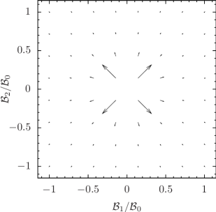
Figure 3: Visualisation of the P-conserving flux-density vector field $\hat{\bm{J}}_{\alpha}^{(\bm{\mathcal{B}})\mathrm{PC}}(\bm{0},\bm{\mathcal{B}})$ (121) for $\alpha=11$ and $\eta=10^{-2}$ in magnetic field parameter space at $\mathcal{B}_{3}=0$.

For any curve $\mathcal{C}=\partial\mathcal{F}$ in $\bm{\mathcal{B}}$ space we get for the geometric phases from (66) and (118)

$$\gamma_{\alpha}(\mathcal{C}) =\int_{\mathcal{F}}\bm{J}_{\alpha}^{(\bm{\mathcal{B}})}(\bm{\mathcal{B}})\,\mathrm{d}\bm{f}^{(\bm{\mathcal{B}})}$$

$$=\left\{\begin{array}[]{cl}-\Omega_{\mathcal{C}}&,\quad\mbox{for }\alpha=9\ ,\\[3.00003pt] +\Omega_{\mathcal{C}}&,\quad\mbox{for }\alpha=11\ ,\\[3.00003pt] 0&,\quad\mbox{for }\alpha=10,12\ .\end{array}\right.$$ (125)

Here $\Omega_{\mathcal{C}}$ is the solid angle spanned by the curve $\mathcal{C}$. This is in accord with the expectation for a spin $1$ system; see Bar83 .

5.2 An electric field $\bm{\mathcal{E}}$ together with a constant magnetic field

We now consider the case of geometric flux densities in electric field space with a constant magnetic field $\bm{\mathcal{B}}=\mathcal{B}_{3}\,\bm{e}_{3}$ with $\mathcal{B}_{3}>0$. Here we find from (107)

$$\bm{J}_{\alpha}^{(\bm{\mathcal{E}})\mathrm{PC}}(\bm{\mathcal{E}},\mathcal{B}_{3}\,\bm{e}_{3}) =\bm{\mathcal{E}}\,\mathcal{E}_{3}\mathcal{B}_{3}\,g^{\alpha}_{1}+\mathcal{B}_{3}\left(\begin{array}[]{c}\mathcal{E}_{2}\mathcal{E}_{3}\mathcal{B}_{3}\,g_{3}^{\alpha}\\ -\mathcal{E}_{1}\mathcal{E}_{3}\mathcal{B}_{3}\,g_{3}^{\alpha}\\ g_{2}^{\alpha}\end{array}\right)\ ,$$ (129)

$$\bm{J}_{\alpha}^{(\bm{\mathcal{E}})\mathrm{PV}}(\bm{\mathcal{E}},\mathcal{B}_{3}\,\bm{e}_{3}) =\bm{\mathcal{E}}\,h_{1}^{\alpha}+\mathcal{B}_{3}\,\bm{e}_{3}\,\mathcal{E}_{3}\mathcal{B}_{3}\,h_{2}^{\alpha}$$

$$\quad+(\mathcal{E}_{2}\,\bm{e}_{1}-\mathcal{E}_{1}\,\bm{e}_{3})\,\mathcal{B}_{3}\,h_{3}^{\alpha}$$

$$=\bm{\mathcal{E}}\,h_{1}^{\alpha}+\mathcal{B}_{3}\left(\begin{array}[]{c}\mathcal{E}_{2}\,h_{3}^{\alpha}\\ -\mathcal{E}_{1}\,h_{3}^{\alpha}\\ \mathcal{E}_{3}\mathcal{B}_{3}\,h_{2}^{\alpha}\end{array}\right)\ ,$$ (133)

where $g_{1,2,3}^{\alpha}$ and $h_{1,2,3}^{\alpha}$ may in general depend on $\bm{\mathcal{E}}^{2}$, $\mathcal{B}_{3}^{2}$ and $(\mathcal{E}_{3}\mathcal{B}_{3})^{2}$ and $\alpha\in\{9,10,11,12\}$. In our case $\mathcal{B}_{3}$ is constant. We have, therefore,

$$g_{i}^{\alpha} =g_{i}^{\alpha}(\bm{\mathcal{E}}_{T}^{2},\mathcal{E}_{3}^{2})\ ,$$

$$h_{i}^{\alpha} =h_{i}^{\alpha}(\bm{\mathcal{E}}_{T}^{2},\mathcal{E}_{3}^{2})\ ,$$

$$(i =1,2,3)$$ (134)

with

$$\bm{\mathcal{E}}_{T}^{2}=\mathcal{E}_{1}^{2}+\mathcal{E}_{2}^{2}\ .$$ (135)

In the following we give the results of numerical evaluations of the PC and PV flux-density vectors (129) and (133), respectively. We split the PV vectors into the contributions from the nuclear-spin independent ($i=1$) and dependent ($i=2$) PV interactions

$$\bm{J}^{(\bm{\mathcal{E}})\mathrm{PV}}=\bm{J}^{(\bm{\mathcal{E}})\mathrm{PV}_{1}}+\bm{J}^{(\bm{\mathcal{E}})\mathrm{PV}_{2}}\ .$$ (136)

Here the $\bm{J}^{(\bm{\mathcal{E}})\mathrm{PV}_{i}}$ are defined as in (4.2) but with $\delta$ replaced by $\delta_{i}$ and $\underline{\mathscr{M}}_{\mathrm{PV}}$ replaced by $\underline{\mathscr{M}}_{\mathrm{PV}}^{(i)}$ ($i=1,2$); see (A.5) and (A). Again we shall plot dimensionless vectors

$$\hat{\bm{J}}_{\alpha}^{(\bm{\mathcal{E}})\mathrm{PC}}(\bm{\mathcal{E}},\mathcal{B}_{3}\,\bm{e}_{3}) =\eta_{\alpha}\,\bm{J}_{\alpha}^{(\bm{\mathcal{E}})\mathrm{PC}}(\bm{\mathcal{E}},\mathcal{B}_{3}\,\bm{e}_{3})\,\mathcal{E}_{0}^{2}\ ,$$ (137)

$$\hat{\bm{J}}_{\alpha}^{(\bm{\mathcal{E}})\mathrm{PV}_{i}}(\bm{\mathcal{E}},\mathcal{B}_{3}\,\bm{e}_{3}) =\eta^{\prime}_{\alpha,i}\,\bm{J}_{\alpha}^{(\bm{\mathcal{E}})\mathrm{PV}_{i}}(\bm{\mathcal{E}},\mathcal{B}_{3}\,\bm{e}_{3})\,\mathcal{E}_{0}^{2}$$ (138)

with $\mathcal{E}_{0}$ from (5.1) and $\eta_{\alpha}$ and $\eta^{\prime}_{\alpha,i}$ conveniently chosen.

As an example of a PC flux-density vector field we present in Figure 4 the results of a numerical calculation of $\bm{J}_{9}^{(\bm{\mathcal{E}})\mathrm{PC}}(\bm{\mathcal{E}},\mathcal{B}_{3}\,\bm{e}_{3})$ for $\mathcal{B}_{3}=1\,\mathrm{mT}$. We recall that the state with $\alpha=9$ is connected to the 2S state with $(F,F_{3})=(1,1)$; see Appendix A. We plot the dimensionless vectors (137) with the scaling factor chosen as $\eta_{9}=2.5\times 10^{4}$. Comparing with (129) we see that here the dominant term is the one proportional to $g_{2}^{\alpha}$:

$$\bm{J}_{9}^{(\bm{\mathcal{E}})\mathrm{PC}}(\bm{\mathcal{E}},\mathcal{B}_{3}\,\bm{e}_{3})\approx\mathcal{B}_{3}\,g_{2}^{9}(\bm{\mathcal{E}}_{T}^{2},\mathcal{E}_{3}^{2})\,\bm{e}_{3}$$ (139)

with $g_{2}^{9}(\bm{\mathcal{E}}_{T}^{2},\mathcal{E}_{3}^{2})$ being practically constant.

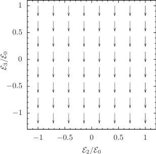
Figure 4: Visualisation of the real part of the P-conserving flux-density vector field $\hat{\bm{J}}_{9}^{(\bm{\mathcal{E}})\mathrm{PC}}(\bm{\mathcal{E}},\mathcal{B}_{3}\,\bm{e}_{3})$ (137) in electric field parameter space at $\mathcal{E}_{1}=1\,\mathrm{V/cm}$. A constant magnetic field with $\mathcal{B}_{3}=1\,\mathrm{mT}$ is applied. The scaling factor in (137) is chosen as $\eta_{9}=2.5\times 10^{4}$.

The numerical results shown in Figure 4 reveal a large sensitivity of the flux-density vector field $\bm{J}_{9}^{(\bm{\mathcal{E}})\mathrm{PC}}$ to the normalisation of the dipole operator $\underline{\bm{D}}$. Indeed, suppose that we make in our calculations the replacement

$$\underline{\bm{D}}\rightarrow\lambda\underline{\bm{D}}$$ (140)

with $\lambda$ a positive real constant. From the mass matrix (2) and from $\mathcal{I}_{9}^{(\bm{\mathcal{E}})}$ in (77) we find the following scaling behaviour for $\bm{J}_{9}^{(\bm{\mathcal{E}})\mathrm{PC}}$

$$\left.\bm{J}_{9}^{(\bm{\mathcal{E}})\mathrm{PC}}(\bm{\mathcal{E}},\mathcal{B}_{3}\,\bm{e}_{3})\right|_{\lambda\underline{\bm{D}}}=\lambda^{2}\left.\bm{J}_{9}^{(\bm{\mathcal{E}})\mathrm{PC}}(\lambda\bm{\mathcal{E}},\mathcal{B}_{3}\,\bm{e}_{3})\right|_{\underline{\bm{D}}}\ .$$ (141)

Since our calculations show that $\bm{J}_{9}^{(\bm{\mathcal{E}})\mathrm{PC}}$ is practically constant for the range of fields explored here we get

$$\left.\bm{J}_{9}^{(\bm{\mathcal{E}})\mathrm{PC}}(\bm{\mathcal{E}},\mathcal{B}_{3}\,\bm{e}_{3})\right|_{\lambda\underline{\bm{D}}}\approx\lambda^{2}\left.\bm{J}_{9}^{(\bm{\mathcal{E}})\mathrm{PC}}(\bm{\mathcal{E}},\mathcal{B}_{3}\,\bm{e}_{3})\right|_{\underline{\bm{D}}}\ .$$ (142)

Therefore, measurements of $\bm{J}_{9}^{(\bm{\mathcal{E}})\mathrm{PC}}(\bm{\mathcal{E}},\mathcal{B}_{3}\,\bm{e}_{3})$ for the setup considered here are highly sensitive to deviations of the normalisation of $\underline{\bm{D}}$ from the standard expression as given in Table 4.

As an example we calculate the PC geometric phase for the following path in $\bm{\mathcal{E}}$ space

$$\mathcal{C}:\;z\rightarrow\bm{\mathcal{E}}(z) =\left(\begin{array}[]{c}1.0+0.5\times\sin(200\,\pi\,z)\\ 0.5\times\cos(200\,\pi\,z)\\ 1.0\end{array}\right)\,\mathrm{V/cm}\ ,$$ (146)

$$z \in[0,1]\ .$$ (147)

That is, we consider a path circling $100$ times in the $\mathcal{E}_{1}-\mathcal{E}_{2}$ plane which is orthogonal to the flux direction for $\alpha=9$; see (139) and Figure 4. For the constant magnetic field chosen there, $\mathcal{B}_{3}=1\,\mathrm{mT}$, we obtain for $\alpha=9$

$$\gamma_{9}(\mathcal{C}) =5.89\times 10^{-4}-5.25\times 10^{-5}\,\mathrm{i}\ .$$ (148)

Decreasing the constant magnetic field $\mathcal{B}_{3}$ we get larger geometric phases. Numerical results of the flux-density vector field $\bm{J}_{9}^{(\bm{\mathcal{E}})\mathrm{PC}}(\bm{\mathcal{E}},\mathcal{B}_{3}\,\bm{e}_{3})$ for $\mathcal{B}_{3}=1\,\mu\mathrm{T}$ are presented in Figure 5. There, the scaling factor is chosen as $\eta_{9}=450$. For the curve (146), $\mathcal{B}_{3}=1\,\mu\mathrm{T}$, and $\alpha=9$ we obtain

$$\gamma_{9}(\mathcal{C}) =0.0340-0.00596\,\mathrm{i}\ .$$ (149)

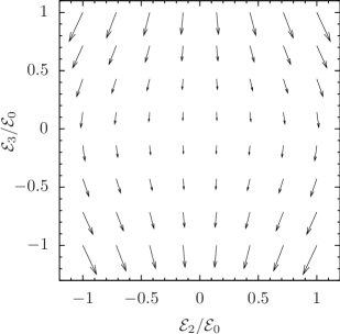
Figure 5: Visualisation of the real part of the P-conserving flux-density vector field $\hat{\bm{J}}_{9}^{(\bm{\mathcal{E}})\mathrm{PC}}(\bm{\mathcal{E}},\mathcal{B}_{3}\,\bm{e}_{3})$ (137) in electric field parameter space at $\mathcal{E}_{1}=1\,\mathrm{V/cm}$. A constant magnetic field with $\mathcal{B}_{3}=1\,\mu\mathrm{T}$ is applied. The scaling factor in (137) is chosen as $\eta_{9}=450$.

As an example of a PV flux-density vector field we present the numerical results for $\bm{J}_{9}^{(\bm{\mathcal{E}})\mathrm{PV}_{2}}$ in Figure 6.

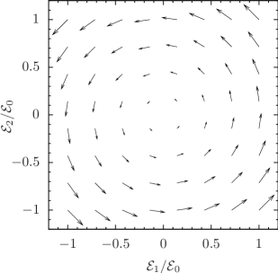
Figure 6: Visualisation of the real part of the nuclear spin dependent P-violating flux-density vector field $\hat{\bm{J}}_{9}^{(\bm{\mathcal{E}})\mathrm{PV}_{2}}(\bm{\mathcal{E}},\bm{\mathcal{B}})$ (138) in electric field parameter space at $\mathcal{E}_{3}=1\,\mathrm{V/cm}$ with an additional constant magnetic field $\bm{\mathcal{B}}=\mathcal{B}_{3}\,\bm{e}_{3}$, $\mathcal{B}_{3}=1\,\mu\mathrm{T}$. The scaling factor in (138) is chosen as $\eta^{\prime}_{9,2}=400/\delta_{2}$.

We find both, the real and the imaginary part of $\bm{J}_{9}^{(\bm{\mathcal{E}})\mathrm{PV}_{2}}(\bm{\mathcal{E}},\mathcal{B}_{3}\,\bm{e}_{3})$ to represent a flow, circulating around the $\bm{e}_{3}$-axis, with vanishing third component. That is, in (133) for $\alpha=9$ the terms involving $h_{1}^{9}$ and $h_{2}^{9}$, respectively, come out numerically to be negligible compared to the terms involving $h_{3}^{9}$. We may hence write

$$\bm{J}_{9}^{(\bm{\mathcal{E}})\mathrm{PV}_{2}}(\bm{\mathcal{E}},\mathcal{B}_{3}\,\bm{e}_{3}) \approx\mathcal{B}_{3}\,h_{3}^{9}(\bm{\mathcal{E}}_{T}^{2},\mathcal{E}_{3}^{2})\left(\begin{array}[]{c}\mathcal{E}_{2}\\ -\mathcal{E}_{1}\\ 0\end{array}\right)\ .$$ (153)

This is corroborated by numerical studies. For $|\mathcal{E}_{j}|\leq\mathcal{E}_{0}$ $(j=1,2,3)$ with $\mathcal{E}_{0}$ from (5.1) we find

$$\frac{|\mathrm{Re}\,\bm{e}_{3}\,\bm{J}_{9}^{(\bm{\mathcal{E}})\mathrm{PV}_{2}}|}{|\mathrm{Re}\,\bm{J}_{9}^{(\bm{\mathcal{E}})\mathrm{PV}_{2}}|}\lesssim 6\times 10^{-11}$$ (154)

and

$$\frac{|\mathcal{E}_{1}\,\mathrm{Re}\,\bm{e}_{1}\,\bm{J}_{9}^{(\bm{\mathcal{E}})\mathrm{PV}_{2}}+\mathcal{E}_{2}\,\mathrm{Re}\,\bm{e}_{2}\,\bm{J}_{9}^{(\bm{\mathcal{E}})\mathrm{PV}_{2}}|}{|\mathrm{Re}\,\bm{J}_{9}^{(\bm{\mathcal{E}})\mathrm{PV}_{2}}|\,\sqrt{\mathcal{E}_{1}^{2}+\mathcal{E}_{2}^{2}}}\lesssim 2.5\times 10^{-11}\ .$$ (155)

Results similar to (154) and (155) hold for the imaginary part $\mathrm{Im}\,\bm{J}_{9}^{(\bm{\mathcal{E}})\mathrm{PV}_{2}}(\bm{\mathcal{E}},\mathcal{B}_{3}\,\bm{e}_{3})$ and for $\bm{J}_{9}^{(\bm{\mathcal{E}})\mathrm{PV}_{1}}(\bm{\mathcal{E}},\mathcal{B}_{3}\,\bm{e}_{3})$. Thus, also $\bm{J}_{9}^{(\bm{\mathcal{E}})\mathrm{PV}_{1}}$ has to a good approximation the structure (153).

The antisymmetry of $\mathrm{Re}\,\bm{J}_{9}^{(\bm{\mathcal{E}})\mathrm{PV}_{2}}(\bm{\mathcal{E}},\mathcal{B}_{3}\,\bm{e}_{3})$ with respect to $\bm{\mathcal{E}}\rightarrow-\bm{\mathcal{E}}$, see (133), is confirmed numerically at the same level of accuracy. We find

$$\left|\frac{|\mathrm{Re}\,\bm{J}_{9}^{(\bm{\mathcal{E}})\mathrm{PV}_{2}}(\bm{\mathcal{E}},\mathcal{B}_{3}\,\bm{e}_{3})|}{|\mathrm{Re}\,\bm{J}_{9}^{(\bm{\mathcal{E}})\mathrm{PV}_{2}}(-\bm{\mathcal{E}},\mathcal{B}_{3}\,\bm{e}_{3})|}-1\right|\lesssim 2.5\times 10^{-10}$$ (156)

and

$$\qquad\frac{|\mathrm{Re}\,\bm{J}_{9}^{(\bm{\mathcal{E}})\mathrm{PV}_{2}}(\bm{\mathcal{E}},\mathcal{B}_{3}\,\bm{e}_{3})+\mathrm{Re}\,\bm{J}_{9}^{(\bm{\mathcal{E}})\mathrm{PV}_{2}}(-\bm{\mathcal{E}},\mathcal{B}_{3}\,\bm{e}_{3})|}{|\mathrm{Re}\,\bm{J}_{9}^{(\bm{\mathcal{E}})\mathrm{PV}_{2}}(\bm{\mathcal{E}},\mathcal{B}_{3}\,\bm{e}_{3})|}$$

$$\lesssim 2.5\times 10^{-10}.$$ (157)

Similar numerical results are also obtained for $\mathrm{Im}\,\bm{J}_{9}^{(\bm{\mathcal{E}})\mathrm{PV}_{2}}(\bm{\mathcal{E}},\mathcal{B}_{3}\,\bm{e}_{3})$ and for the real and imaginary parts of $\bm{J}_{9}^{(\bm{\mathcal{E}})\mathrm{PV}_{1}}(\bm{\mathcal{E}},\mathcal{B}_{3}\,\bm{e}_{3})$.

5.3 The mixed parameter space of $\mathcal{E}_{1}$, $\mathcal{E}_{3}$, $\mathcal{B}_{3}$ together with a constant magnetic field

In our last example we discuss the parameter space spanned by the vectors

$$\bm{L}\equiv\left(\begin{array}[]{c}L_{1}\\ L_{2}\\ L_{3}\end{array}\right)=\left(\begin{array}[]{ccc}\mathcal{E}_{0}^{-1}&0&0\\ 0&\mathcal{E}_{0}^{-1}&0\\ 0&0&\mathcal{B}_{0}^{-1}\\ \end{array}\right)\left(\begin{array}[]{c}\mathcal{E}_{1}\\ \mathcal{E}_{3}\\ \mathcal{B}_{3}\end{array}\right)\ ,$$ (167)

see (60) ff. and (5.1). In addition we assume the presence of a constant magnetic field $\bm{\mathcal{B}}=1\,\mu\mathrm{T}\,\bm{e}_{2}$. The values chosen for $\mathcal{E}_{0}$ and $\mathcal{B}_{0}$ in (5.1) and (167) should represent the typical range of electric and magnetic field variations, respectively, for a given experiment. Our choice here is motivated by the discussion of the longitudinal spin echo experiments in BeGaMaNaTr08_I . For other experiments different choices of $\mathcal{E}_{0}$ and $\mathcal{B}_{0}$ will be appropriate.

From (60), (3), and (77) to (83) we find

$$\bm{J}_{\alpha}^{(\bm{L})}(\bm{\mathcal{E}},\bm{\mathcal{B}})=\left(\begin{array}[]{ccc}\mathcal{E}_{0}\mathcal{B}_{0}&0&0\\ 0&\mathcal{E}_{0}\mathcal{B}_{0}&0\\ 0&0&\mathcal{E}_{0}^{2}\\ \end{array}\right)\left(\begin{array}[]{c}\mathcal{I}_{\alpha,33}^{(\bm{\mathcal{E}},\bm{\mathcal{B}})}(\bm{\mathcal{E}},\bm{\mathcal{B}})\\ -\mathcal{I}_{\alpha,13}^{(\bm{\mathcal{E}},\bm{\mathcal{B}})}(\bm{\mathcal{E}},\bm{\mathcal{B}})\\ 2\,\mathcal{I}_{\alpha,13}^{(\bm{\mathcal{E}})}(\bm{\mathcal{E}},\bm{\mathcal{B}})\end{array}\right)\ .$$ (174)

Here again $\alpha\in\{9,10,11,12\}$ labels the metastable state, see Table 2 of Appendix A, to which the geometric flux density corresponds. Inserting in (174) the expressions from (107) and (108) we get for the PC and PV parts of $\bm{J}_{\alpha}^{(\bm{L})}(\bm{\mathcal{E}},\bm{\mathcal{B}})$

$$\bm{J}_{\alpha}^{(\bm{L})\mathrm{PC}}(\bm{\mathcal{E}},\bm{\mathcal{B}}) =\left(\begin{array}[]{c}\mathcal{B}_{3}\mathcal{E}_{3}\,\tilde{g}_{1}^{\alpha}+\mathcal{B}_{3}\mathcal{E}_{1}\,\tilde{g}_{2}^{\alpha}\\ \mathcal{B}_{3}\mathcal{E}_{3}\,\tilde{g}_{3}^{\alpha}+\mathcal{B}_{3}\mathcal{E}_{1}\,\tilde{g}_{4}^{\alpha}\\ \tilde{g}_{5}^{\alpha}+\mathcal{E}_{1}\mathcal{E}_{3}\,\tilde{g}_{6}^{\alpha}\end{array}\right)\ ,$$ (178)

$$\bm{J}_{\alpha}^{(\bm{L})\mathrm{PV}}(\bm{\mathcal{E}},\bm{\mathcal{B}}) =\left(\begin{array}[]{c}\tilde{h}_{1}^{\alpha}+\mathcal{E}_{1}\mathcal{E}_{3}\,\tilde{h}_{2}^{\alpha}\\ \tilde{h}_{3}^{\alpha}+\mathcal{E}_{1}\mathcal{E}_{3}\,\tilde{h}_{4}^{\alpha}\\ \mathcal{B}_{3}\mathcal{E}_{3}\,\tilde{h}_{5}^{\alpha}+\mathcal{B}_{3}\mathcal{E}_{1}\,\tilde{h}_{6}^{\alpha}\end{array}\right)\ ,$$ (182)

where the functions $\tilde{g}_{i}^{\alpha}$ and $\tilde{h}_{i}^{\alpha}$, $i\in\{1,\dots,6\}$, may in general depend on $\mathcal{E}_{1}^{2}$, $\mathcal{E}_{3}^{2}$ and $\mathcal{B}_{3}^{2}$; see Appendix D.

For ease of graphical presentation we shall multiply the $\bm{J}_{\alpha}^{(\bm{L})}$ with scaling factors $\eta$. Thus we define

$$\hat{\bm{J}}_{\alpha}^{(\bm{L})\mathrm{PC}}(\bm{\mathcal{E}},\bm{\mathcal{B}}) =\eta_{\alpha}\,\bm{J}_{\alpha}^{(\bm{L})\mathrm{PC}}(\bm{\mathcal{E}},\bm{\mathcal{B}})\ ,$$ (183)

$$\hat{\bm{J}}_{\alpha}^{(\bm{L})\mathrm{PV}_{i}}(\bm{\mathcal{E}},\bm{\mathcal{B}}) =\eta_{\alpha,i}^{\prime}\,\bm{J}_{\alpha}^{(\bm{L})\mathrm{PV}_{i}}(\bm{\mathcal{E}},\bm{\mathcal{B}})\ ,$$

$$(i =1,2)\ .$$ (184)

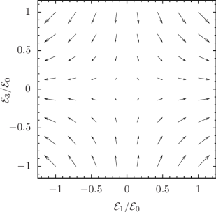
Figure 7: Visualisation of the 1 and 2 components of the real part of the P-conserving flux-density vector field $\hat{\bm{J}}_{9}^{(\bm{L})\mathrm{PC}}(\bm{\mathcal{E}},\bm{\mathcal{B}})$ (183) at $\mathcal{B}_{3}=143\,\mu\mathrm{T}$. The scaling factor is chosen as $\eta_{9}=2.5\times 10^{4}$.

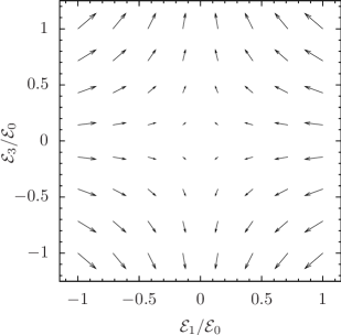
Figure 8: Visualisation of the 1 and 2 components of the imaginary part of the P-conserving flux-density vector field $\hat{\bm{J}}_{9}^{(\bm{L})\mathrm{PC}}(\bm{\mathcal{E}},\bm{\mathcal{B}})$ (183) at $\mathcal{B}_{3}=143\,\mu\mathrm{T}$. The scaling factor is chosen as $\eta_{9}=2.7\times 10^{5}$.

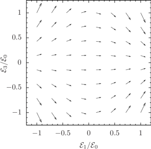
Figure 9: Visualisation of the 1 and 2 components of the real part of the nuclear spin dependent P-violating flux-density vector field $\hat{\bm{J}}_{9}^{(\bm{L})\mathrm{PV}_{2}}(\bm{\mathcal{E}},\bm{\mathcal{B}})$ (184) at $\mathcal{B}_{3}=143\,\mu\mathrm{T}$. The scaling factor is chosen as $\eta_{9,2}^{\prime}=10^{4}/\delta_{2}$.

Figure 10: Visualisation of the 1 and 2 components of the real part of the nuclear spin dependent P-violating flux-density vector field $\hat{\bm{J}}_{9}^{(\bm{L})\mathrm{PV}_{2}}(\bm{\mathcal{E}},\bm{\mathcal{B}})$ (184) at $\mathcal{B}_{3}=86\,\mu\mathrm{T}$. The scaling factor is chosen as $\eta_{9,2}^{\prime}=4\times 10^{3}/\delta_{2}$.

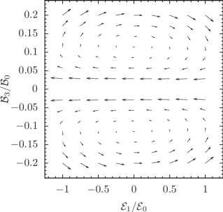
Figure 11: Visualisation of the 1 and 3 components of the real part of the nuclear spin dependent P-violating flux-density vector field $\hat{\bm{J}}_{9}^{(\bm{L})\mathrm{PV}_{2}}(\bm{\mathcal{E}},\bm{\mathcal{B}})$ (184) at $\mathcal{E}_{3}=0$. In order to resolve the structure more clearly the scaling factor is chosen as $\eta_{9,2}^{\prime}=2\times 10^{5}\,|\mathcal{B}_{3}/\mathcal{B}_{0}|^{2}/\delta_{2}$.

In the Figures 7 to 11 we illustrate the results of our numerical calculations of (183) and (184) for the geometric flux densities of the state with $\alpha=9$, that is, the state connected with the 2S, $(F,F_{3})=(1,1)$ state; see Appendix A, Table 2. For $30^{3}$ grid points in the parameter space volume $[-\mathcal{E}_{0},\mathcal{E}_{0}]^{2}\times[-0.2\mathcal{B}_{0},0.2\mathcal{B}_{0}]$ we find that numerically

$$|\mathrm{Re}\,\bm{e}_{3}\,\hat{\bm{J}}_{9}^{(\bm{L})\mathrm{PC}}| \lesssim 0.2\,\Big{[}(\mathrm{Re}\,\bm{e}_{1}\,\hat{\bm{J}}_{9}^{(\bm{L})\mathrm{PC}})^{2}$$

$$\qquad\qquad+(\mathrm{Re}\,\bm{e}_{2}\,\hat{\bm{J}}_{9}^{(\bm{L})\mathrm{PC}})^{2}\Big{]}^{\frac{1}{2}}\ .$$ (185)

An analogous relation holds for $\mathrm{Im}\,\hat{\bm{J}}_{9}^{(\bm{L})\mathrm{PC}}(\bm{\mathcal{E}},\bm{\mathcal{B}})$. This justifies the presentation of these flux-density vector fields in the $\mathcal{E}_{1}-\mathcal{E}_{3}$ plane as representative vector field structures. Investigating the dependencies of $\bm{J}_{9}^{(\bm{L})}(\bm{\mathcal{E}},\bm{\mathcal{B}})$ on $\mathcal{E}_{1}$, $\mathcal{E}_{3}$ and $\mathcal{B}_{3}$ we find our numerical results to be consistent with the analytic structures in (178) and (182). We recall from (67) that $\hat{\bm{J}}_{9}^{(\bm{L})\mathrm{PC}}$ is divergence free and, thus, generated by a non-vanishing vortex distribution $\mathrm{rot}\,\bm{J}_{9}^{(\bm{L})\mathrm{PC}}$. We have calculated this quantity numerically using (3) and find $\mathrm{rot}\,\bm{J}_{9}^{(\bm{L})\mathrm{PC}}$ to be in agreement with a direct evaluation using a fit function representing $\hat{\bm{J}}_{9}^{(\bm{L})\mathrm{PC}}$.

Examples of PV flux-density vector fields are shown in Figures 9 to 11. Again, the full three-dimensional vector fields are divergence free and thus represent flows without sources or sinks. Note that in Figure 11 we have chosen a scaling factor depending on $\mathcal{B}_{3}$ since the magnitude of the vector $\bm{J}_{9}^{(\bm{L})\mathrm{PV}_{2}}(\bm{\mathcal{E}},\bm{\mathcal{B}})$ shows a strong increase towards $\mathcal{B}_{3}=0$.

The emergence of non-vanishing imaginary parts of the flux-density vector fields, for example, in the parameter space considered in the present section, see Figure 8, leads to an interesting phenomenon. Let us consider a closed curve $\mathcal{C}$, being the boundary of a surface $\mathcal{F}$, in $\bm{L}$ space (167). We parametrise $\mathcal{C}$ as

$$\mathcal{C}:\; z\rightarrow\bm{L}(z)\ ,$$

$$0\leq z\leq 1\ ,$$

$$\bm{L}(0)=\bm{L}(1)\ ,$$ (186)

cf. (35), (37). We suppose that over a time interval $[0,T]$ this curve in parameter space is run through by the system in the following way:

$$t\rightarrow z(t)=\frac{t}{T}\ ,$$

$$0\leq t\leq T\ ,$$

$$\mathcal{C}:\; t\rightarrow\bm{L}(z(t))\ .$$ (187)

We consider the adiabatic limit where $T$ becomes very large. We shall also consider that the system is run through the curve $\mathcal{C}$ in the reverse direction:

$$t\rightarrow\bar{z}(t)=\frac{T-t}{T}=1-z(t)\ ,$$

$$0\leq t\leq T\ ,$$

$$\bar{\mathcal{C}}:\; t\rightarrow\bm{L}(\bar{z}(t))\ .$$ (188)

Suppose now that we have at $t=0$ the atom in the initial state $\psi_{\alpha}(0)$, see (31). We change the parameters $\bm{L}$ along the curve $\mathcal{C}$ as in (5.3). From (31) to (33) we find the decrease of the norm of the state at time $T$ to be

$$\frac{|\psi_{\alpha}(T)|^{2}}{|\psi_{\alpha}(0)|^{2}}=\exp\left[+2\,\mathrm{Im}\,\varphi_{\alpha}(T)-2\,\mathrm{Im}\,\gamma_{\alpha}(T)\right]\ .$$ (189)

Here $2\,\mathrm{Im}\,\varphi_{\alpha}(T)$ and $2\,\mathrm{Im}\,\gamma_{\alpha}(T)$ are the contributions due to the dynamic and geometric phases, respectively,

$$2\,\mathrm{Im}\,\varphi_{\alpha}(T) =T\,2\,\mathrm{Im}\,\int_{0}^{1}\mathrm{d}z\,E_{\alpha}(\bm{L}(z))\ ,$$

$$2\,\mathrm{Im}\,\gamma_{\alpha}(T) =2\,\mathrm{Im}\,\int_{\mathcal{F}}\bm{J}_{\alpha}^{(\bm{L})}(\bm{L})\,\mathrm{d}\bm{f}^{\bm{L}}\ ;$$ (190)

see (3) and (66). From (189) we can define an effective decay rate for the state $\alpha$ under the above conditions as

$$\Gamma_{\alpha,\mathrm{eff}}(\mathcal{C},T) =\frac{1}{T}\left[-2\,\mathrm{Im}\,\varphi_{\alpha}(T)+2\,\mathrm{Im}\,\gamma_{\alpha}(T)\right]$$

$$=-2\,\mathrm{Im}\,\int_{0}^{1}\mathrm{d}z\,E_{\alpha}(\bm{L}(z))$$

$$\qquad+\frac{2}{T}\,\mathrm{Im}\,\int_{\mathcal{F}}\bm{J}_{\alpha}^{(\bm{L})}(\bm{L})\,\mathrm{d}\bm{f}^{\bm{L}}\ .$$ (191)

Note that this effective decay rate depends, of course, on the curve $\mathcal{C}$ and that the geometric contribution is suppressed by a factor $1/T$ relative to the dynamic contribution. From (189) and (5.3) we get for the decrease of the norm of the state

$$\frac{|\psi_{\alpha}(T)|^{2}}{|\psi_{\alpha}(0)|^{2}}=\exp\left[-\Gamma_{\alpha,\mathrm{eff}}(\mathcal{C},T)\,T\right]\ .$$ (192)

Now we start again with the state $\psi_{\alpha}(0)$ at time $t=0$ but we change the parameters $\bm{L}$ along the reverse curve $\bar{\mathcal{C}}$ (5.3). It is easy to see that the dynamic term in (5.3) does not change whereas the geometric term changes sign,

$$\Gamma_{\alpha,\mathrm{eff}}(\bar{\mathcal{C}},T) =-2\,\mathrm{Im}\int_{0}^{1}\mathrm{d}z\,E_{\alpha}(\bm{L}(z))$$

$$\qquad-\frac{2}{T}\,\mathrm{Im}\,\int_{\mathcal{F}}\bm{J}_{\alpha}^{(\bm{L})}(\bm{L})\,\mathrm{d}\bm{f}^{\bm{L}}\ .$$ (193)

Thus, the effective decay rate depends on the geometry and reversing the sense of the running through our closed curve in parameter space changes the sign of the geometric part.

As a concrete example we choose a constant magnetic field $\mathcal{B}_{2}\,\bm{e}_{2}$ with $\mathcal{B}_{2}=1\,\mu\mathrm{T}$ and the following curve in $\bm{L}$ space

$$\mathcal{C}:\;z\rightarrow\bm{L}(z) =\left(\begin{array}[]{c}\mathcal{E}_{1}(z)/\mathcal{E}_{0}\\ \mathcal{E}_{3}(z)/\mathcal{E}_{0}\\ \mathcal{B}_{3}(z)/\mathcal{B}_{0}\end{array}\right)\ ,$$ (197)

$$\mathcal{E}_{1}(z) =0.8\,\mathrm{V/cm}\ ,$$

$$\mathcal{E}_{3}(z) =0.5\times\cos(4\,\pi\,z)\,\mathrm{V/cm}\ ,$$

$$\mathcal{B}_{3}(z) =[2+2\times\sin(4\,\pi\,z)]\,\mu\mathrm{T}\ ,$$

$$0 \leq z\leq 1\ ;$$ (198)

see Figure 12.

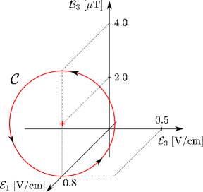
Figure 12: The curve $\mathcal{C}$ (197) in the parameter space $\mathcal{E}_{1},\,\mathcal{E}_{3},\,\mathcal{B}_{3}$. The circle is run through twice.

We suppose as in (5.3) that $\mathcal{C}$ is run through in a time $T$ with $z(t)=t/T$. In this time the path in parameter space makes, according to (197), two loops. With $T=1\,\mathrm{ms}$ we can meet the adiabaticity requirements as spelt out in BeGaMaNaTr08_I and in Equations (30), (31), and (37) of BeGaNa07_II . The essential requirement here is that the frequency $\nu=2/T$ of the external field variation in (197) must be much less than the transition frequencies $\Delta E/h$ between the Zeeman levels for $\alpha=9,10,11$. For the external field of order $1\,\mu\mathrm{T}$ we get $\Delta E/h\simeq 10\,\mathrm{kHz}$ which gives the requirement

$$\nu=\frac{2}{T} \ll 10\,\mathrm{kHz}\ ,$$

$$T \gg 0.2\,\mathrm{ms}\ .$$ (199)

Calculating now the contributions to the effective decay rate (5.3) we find for the state $\alpha=9$ which is connected to the 2S state with $(F,F_{3})=(1,1)$, see Appendix A, the following

$$-2\,\mathrm{Im}\int_{0}^{1}\mathrm{d}z\,E_{9}(\bm{L}(z)) =1935.2\,\mathrm{s}^{-1}\ ,$$ (200)

$$\frac{2}{T}\,\mathrm{Im}\int_{\mathcal{F}}\bm{J}_{9}^{(\bm{L})}(\bm{L})\,\mathrm{d}\bm{f}^{\bm{L}} =-1.8\,\mathrm{s}^{-1}\ .$$ (201)

This leads to

$$\Gamma_{9,\mathrm{eff}}(\mathcal{C},T)=1933.4\,\mathrm{s}^{-1}\ .$$ (202)

For the reverse curve $\bar{\mathcal{C}}$ we find, instead,

$$\Gamma_{9,\mathrm{eff}}(\bar{\mathcal{C}},T)=1937.0\,\mathrm{s}^{-1}\ .$$ (203)

Thus, under the above conditions the effective decay rates (202) and (203) differ by $1.9\,\tcperthousand$ and the corresponding decreases of the norms (192) by $3.6\,\tcperthousand$. We emphasise that this difference has its origin in the geometric phase.

To give an example of a PV geometric phase we consider the following curve

$$\mathcal{C}^{\prime}:\;z\rightarrow\bm{L}(z) =\left(\begin{array}[]{c}\mathcal{E}_{1}(z)/\mathcal{E}_{0}\\ \mathcal{E}_{3}(z)/\mathcal{E}_{0}\\ \mathcal{B}_{3}(z)/\mathcal{B}_{0}\end{array}\right)\ ,$$ (207)

$$\mathcal{E}_{1}(z) =0\ ,$$

$$\mathcal{E}_{3}(z) =\mathcal{E}_{0}\,\sin(2\,\pi\,z)\ ,$$

$$\mathcal{B}_{3}(z) =0.1\,\mathcal{B}_{0}\,\cos(2\,\pi\,z)\ ,$$

$$0 \leq z\leq 1\ .$$ (208)

For this curve the PC geometric phases vanish due to the antisymmetry of $\bm{e}_{1}\cdot\bm{J}_{\alpha}^{(\bm{\mathcal{E}})\mathrm{PC}}(\bm{\mathcal{E}},\mathcal{B}_{3}\,\bm{e}_{3})$ under $(\mathcal{E}_{1},\mathcal{E}_{3})\rightarrow(-\mathcal{E}_{1},-\mathcal{E}_{3})$; see (178). Thus, we get here

$$\gamma_{\alpha}(\mathcal{C}^{\prime})=\gamma_{\alpha}^{\mathrm{PV}}(\mathcal{C}^{\prime})=\gamma_{\alpha}^{\mathrm{PV}_{1}}(\mathcal{C}^{\prime})+\gamma_{\alpha}^{\mathrm{PV}_{2}}(\mathcal{C}^{\prime})\ .$$ (209)

Numerically we find for $\alpha=9$ and $\mathcal{B}_{2}=1\,\mu\mathrm{T}$

$$\gamma_{9}^{\mathrm{PV}_{1}}(\mathcal{C}^{\prime}) =(0.00467-0.000457\,\mathrm{i})\,\delta_{1}\ ,$$ (210)

$$\gamma_{9}^{\mathrm{PV}_{2}}(\mathcal{C}^{\prime}) =(0.0942-0.00421\,\mathrm{i})\,\delta_{2}\ .$$ (211)

Assuming now that we can circle the curve $\mathcal{C}^{\prime}$ $N$ times we get as geometric phase $N\gamma_{9}(\mathcal{C}^{\prime})$. Thus, the number of circlings acts as an enhancement factor for the small weak interaction effects in hydrogen. For $N=10^{4}$, for example, we obtain

$$N\gamma_{9}^{\mathrm{PV}}(\mathcal{C}^{\prime}) =(46.7-4.57\,\mathrm{i})\,\delta_{1}+(942-42.1\,\mathrm{i})\,\delta_{2}\ .$$ (212)

With $\delta_{1,2}$ from Table 1 this gives a phase of the order of $10^{-9}$.

6 Conclusions and outlook

In this article we have discussed the geometric phases and flux densities of the metastable states of hydrogen with principal quantum number $n=2$ in the presence of external electric and magnetic fields. We have provided expressions for the flux densities and their derivatives suited for an investigation of their general structure. This was achieved with the help of representations of the flux densities as complex integrals. For these integrals extensive use was made of resolvent methods, and the results turned out to be quite simple and easy to handle. Furthermore, employing proper and improper rotations we derived the general structure of the flux densities for the metastable states. We also obtained expansions of the flux densities in terms of P-conserving and P-violating contributions. The flux densities can be visualised in the case of three-dimensional parameter spaces as vector fields. We gave three examples of parameter spaces for which we compared analytical with numerical calculations. The results are consistent regarding the employed numerical precision. For vanishing electric field the flux densities in magnetic field space are real and P-conserving – and so are the corresponding geometric phases. In this case the flux-density vector field can be computed analytically and turns out to be the field of a Dirac monopole sitting at $\bm{\mathcal{B}}=0$. In parameter spaces of both electric and magnetic field components the flux densities exhibit a rich structure of P-conserving as well as P-violating vector fields including both real and imaginary parts. In the general structures of the flux densities of those cases we encounter functions which are rotationally invariant; see (107) to (109). These functions contain all the information on the mass matrix and the electric and magnetic dipole matrices which one can obtain from the measurement of the geometric phases for the system considered.

In Section 5 we have calculated geometric phases for various situations and, surely, the question arises about their possible measurements. Present experiments can reach a precision in phase measurements of about $10^{-5}\,\mathrm{rad}$ DeKprivcom2 . Thus, the PC phases (5.1), (148), (149) and the change of decay rate (202) and (203) should be within reach of these experiments. The PV phases for hydrogen certainly need further theoretical and experimental efforts to bring them to a practically measurable level.

The general representations for the flux densities as complex integrals are, of course, easily transferred to other atomic systems having stable or metastable states, for instance, to the states of $n=2$ helium. Similarly, the analysis of the consequences of rotational invariance and of P violation in Section 4 goes through unchanged for other atomic systems. The only requirement here is that the coupling of the system to the external electric and magnetic fields can be described as in (2) with electric and magnetic dipole matrices $\underline{\bm{D}}$ and $\underline{\bm{\mu}}$, respectively. We note that measuring geometric phases for such systems can give valuable information on their atomic matrix elements. We have found for hydrogen that, on the one hand, there is the case of a pure magnetic field where the flux densities and geometric phases are simply given by the geometry of the path run through in parameter space; see Section 5.1. On the other hand, a large sensitivity on the electric dipole matrix element was found for the flux densities in electric field space with the presence of a constant magnetic field in Section 5.2. We also discussed the change of the effective decay rates for geometric reasons in Section 5.3. All these phenomena should also occur for other atomic systems. Measurements of geometric phases could be an important testing ground for theoretical calculations of wave functions and matrix elements for atomic systems, for instance, for He.

Acknowledgements

The authors would like to thank M. DeKieviet, G. Lach, P. Schmelcher, and A. Surzhykov for useful discussions. Special thanks are due to M. Diehl for providing us the information on the current status of the strange-quark contribution to the spin of the proton.
This project is partially funded by the Klaus Tschira Foundation gGmbH and supported by the Heidelberg Graduate School of Fundamental Physics and the Deutsche Forschungsgemeinschaft.

Appendices

Appendix A The $n=2$ states of hydrogen

In this appendix we collect the numerical values for the quantities entering our calculations for the hydrogen states with principal quantum number $n=2$. We specify our numbering scheme for these states. The expressions for the mass matrix at zero external fields and for the electric and the magnetic dipole operators are given in Appendix E.

In Table 1 we present for ${}^{1}_{1}$H, where the nuclear spin is $I=1/2$, the numerical values for the weak charges $Q_{W}^{(\varkappa)}$, $\varkappa=1,2$, the quantities $\Delta q+\Delta\bar{q}$, the Lamb shift $L=E(2\mathrm{S}_{1/2})-E(2\mathrm{P}_{1/2})$, the fine structure splitting $\Delta=E(2\mathrm{P}_{3/2})-E(2\mathrm{P}_{1/2})$, and the ground state hyperfine splitting energy $\mathcal{A}$. We have $\mathcal{A}=E(1\mathrm{S}_{1/2},F=1)-E(1\mathrm{S}_{1/2},$ $F=0)$ for hydrogen. We define the weak charges as in Section 2 of BeGaNa07_II which gives for the proton in the standard model (SM):

$$Q_{W}^{(1)} =1-4\sin^{2}\vartheta_{W}\ ,$$

$$Q_{W}^{(2)} =-2\,(1-4\sin^{2}\vartheta_{W})$$

$$\quad\times(\Delta u+\Delta\bar{u}-\Delta d-\Delta\bar{d}-\Delta s-\Delta\bar{s})\ .$$ (A.1)

Here $\vartheta_{W}$ is the weak mixing angle and $\Delta q+\Delta\bar{q}$ denotes the total polarisation of the proton carried by the quarks and antiquarks of species $q$ $(q=u,d,s)$. Note that in BeGaNa07_II and BoBrNa95 we adhered to the then usual notation of $\Delta q$ for what is now denoted as $\Delta q+\Delta\bar{q}$. The quantity $\Delta u+\Delta\bar{u}-\Delta d-\Delta\bar{d}$ is related to the ratio $g_{A}/g_{V}$ from neutron $\beta$ decay:

$$\Delta u+\Delta\bar{u}-\Delta d-\Delta\bar{d}=-g_{A}/g_{V}\ .$$ (A.2)

The numerical value given in Table 1 is from PDG10 . The total polarisation of the proton carried by strange quarks, $\Delta s+\Delta\bar{s}$, is still only poorly known experimentally. One finds values of $-0.12$ to very small and positive ones quoted in recent papers; see for instance PhysRevC.78.015207 ; PhysRevLett.101.072001 ; PhysRevD.80.034030 ; Alekseev2010227 ; Leader2011 . Therefore, we assume for our purposes

$$-0.12\leq\Delta s+\Delta\bar{s}\leq 0\ .$$ (A.3)

Of course, the dependence of $Q_{W}^{(2)}$ on $\Delta s+\Delta\bar{s}$ is, in principle, very interesting, since this quantity can be determined in atomic P violation experiments with hydrogen.

We define (see (19) of BeGaNa07_II ) the dimensionless constants

$$\delta_{\varkappa}=-\frac{\sqrt{3}\,G}{64\pi\sqrt{2}\,r_{B}^{4}m_{e}}\frac{Q_{W}^{(\varkappa)}}{L}\qquad(\varkappa=1,2)$$ (A.4)

with Fermi’s constant $G$, the Bohr radius $r_{B}$ and the electron mass $m_{e}$. We see from Table 1 that varying $\Delta s+\Delta\bar{s}$ in the range (A.3) corresponds to a $10\%$ shift in $\delta_{2}$. Thus, a percent-level measurement of $\delta_{2}$ would be most welcome for a clarification of the role of strange quarks for the nucleon spin.

	${}_{1}^{1}$H		Ref.
$L/h$	1057.8440(24) MHzaaa		NISTData
$\Delta/h$	10969.0416(48) MHzaaa		NISTData
$\mathcal{A}/h$	1420.405751768(1) MHzaaa		Kar05
$Q_{W}^{(1)}$	0.04532(64)		(11) of BeGaNa07_II
$\delta_{1}$	$-2.78(4)\times 10^{-13}$		(20) of BeGaNa07_II
$\Delta u+\Delta\bar{u}$ $-\Delta d-\Delta\bar{d}$	$1.2694(28)$		PDG10
$\Delta s+\Delta\bar{s}$	$-0.12$	$0.00$	(A.3)
$Q_{W}^{(2)}$	$-0.1259(18)$	$-0.1151(16)$	(A)-(A.4)
$\delta_{2}$	$7.74(11)\times 10^{-13}$	$7.07(10)\times 10^{-13}$

Table 1: Values of parameters for ${}^{1}_{1}$H for numerical calculations. The weak mixing angle in the low energy limit, $\sin^{2}\vartheta_{W}=0.23867(16)$, is taken from ErRa05 . The uncertainty in $\delta_{1}$ is dominated by the uncertainty of $\sin^{2}\vartheta_{W}$. The uncertainties quoted for $Q_{W}^{(2)}$ and $\delta_{2}$ for hydrogen are resulting from the error of the weak mixing angle. The variation of $Q_{W}^{(2)}$ and $\delta_{2}$ with $(\Delta s+\Delta\bar{s})$ varying in the range (A.3) is given explicitly.

The mass matrix for zero external fields is given by

$$\underline{\mathscr{\tilde{M}}}_{0}=\underline{\mathscr{M}}_{0}+\delta_{1}\,\underline{\mathscr{M}}_{\mathrm{PV}}^{(1)}+\delta_{2}\,\underline{\mathscr{M}}_{\mathrm{PV}}^{(2)}\ ;$$ (A.5)

see (22) to (24) of BeGaNa07_II and Table 3 in Appendix E below. The terms $\underline{\mathscr{M}}_{\mathrm{PV}}^{(1)}$ and $\underline{\mathscr{M}}_{\mathrm{PV}}^{(2)}$ correspond to the nuclear-spin independent and dependent PV interaction, respectively. As in (C.31) ff. of BeGaNa07_II we define

$$\delta =(\delta_{1}^{2}+\delta_{2}^{2})^{\frac{1}{2}}\ ,$$

$$\underline{\mathscr{M}}_{\mathrm{PV}} =\sum_{i=1}^{2}\frac{\delta_{i}}{\delta}\underline{\mathscr{M}}_{\mathrm{PV}}^{(i)}\ .$$ (A.6)

The $n=2$ states of hydrogen in the absence of P violation and for zero external fields are denoted by $|2L_{J},$ $F,F_{3})$, where $L$, $J$, $F$ and $F_{3}$ are the quantum numbers of the electron’s orbital angular momentum, its total angular momentum, the total atomic angular momentum and its third component, respectively.

To give the matrices $\underline{\mathscr{M}}_{0}$, $\underline{\mathscr{M}}_{\mathrm{PV}}^{(1)}$, $\underline{\mathscr{M}}_{\mathrm{PV}}^{(2)}$, $\underline{\bm{D}}$, and $\underline{\bm{\mu}}$ explicitly we use the following procedure. The hermitian part of $\underline{\mathscr{M}}_{0}$, that is, $(\underline{\mathscr{M}}_{0}+\underline{\mathscr{M}}_{0}^{\dagger})/2$ is given by the known energy levels of the $n=2$ hydrogen states; see Table 1. The decay matrix $\underline{\Gamma}=\mathrm{i}(\underline{\mathscr{M}}_{0}-\underline{\mathscr{M}}_{0}^{\dagger})$ needs a little discussion. We have (for atoms at rest), see for instance (3.13) of BoBrNa95 ,

$$(2L^{\prime}_{J^{\prime}},F^{\prime},F^{\prime}_{3}|\underline{\Gamma}|2L_{J},F,F_{3})=2\pi\sum_{X}\left<\right.{X}\left.\right|{\mathcal{T}}\left|\right.{2L^{\prime}_{J^{\prime}},F^{\prime},F^{\prime}_{3}}\left.\right)^{*}$$

$$\qquad\qquad\qquad\quad\times\delta(E_{X}-E_{2})\left<\right.{X}\left.\right|{\mathcal{T}}\left|\right.{2L_{J},F,F_{3}}\left.\right)\ .$$ (A.7)

Here, $|X\rangle$ denotes the decay states, the atom in a $n=1$ state plus photons, and $\mathcal{T}$ is the transition matrix. Rotational invariance tells us immediately that the matrix $\underline{\Gamma}$ must be diagonal in $(F,F_{3})$. We shall neglect P violation in the decay. Then the non-diagonal matrix elements between S states $(L=0)$ and P states $(L=1)$ must be zero. The only non-diagonal matrix elements (A) which could be non-zero are, therefore, those for $L=L^{\prime}=1$, $F=1$, and $(J^{\prime},J)=(1/2,3/2)$ or $(J^{\prime},J)=(3/2,1/2)$, respectively. But calculating these matrix elements inserting the usual formulae for E1 transitions on the r.h.s. of (A) we get zero. Thus, neglecting higher order corrections, the matrix $\underline{\Gamma}$ (A) is diagonal. The numerical values for the diagonal elements of $\underline{\Gamma}$ are taken from Sap04 ; LaShSo05 .

To calculate the matrices $\underline{\mathscr{M}}_{\mathrm{PV}}^{(1)}$, $\underline{\mathscr{M}}_{\mathrm{PV}}^{(2)}$, $\underline{\bm{D}}$, and $\underline{\bm{\mu}}$ we use the standard Coulomb wave functions for hydrogen. As in BoBrNa95 (see Appendix B there) we use for these states the phase conventions of CoSh63 except for an overall sign change in all radial wave functions. The matrices $\underline{\mathscr{\tilde{M}}}_{0}$, $\underline{D}_{j}$ and $\underline{\mu}_{j}$ in this basis are collected in Tables 3 to 5 of Appendix E (online material only).

Now we discuss the properties, the ordering and the numbering of the eigenstates of $\underline{\mathscr{M}}(\bm{\mathcal{E}},\bm{\mathcal{B}})$ as given in (2).

We are interested only in moderate magnetic fields, that is, we want to stay below the first level crossing in the Breit-Rabi diagram, which implies

$$|\bm{\mathcal{B}}|<53.8\,\mathrm{mT}\ .$$ (A.8)

Note that these crossings are only in the real part of the eigenenergies; see (18). In the region (A.8) degeneracies of the complex energies (18) occur for $\bm{\mathcal{B}}=\bm{0}$ at arbitrary $\bm{\mathcal{E}}$. This is a consequence of time-reversal (T) invariance. For $\bm{\mathcal{B}}=\bm{0}$ and $\bm{\mathcal{E}}\not=\bm{0}$ we can choose the vector $\bm{e}_{3}^{\prime}=\bm{\mathcal{E}}/|\bm{\mathcal{E}}|$ as quantisation axis of angular momentum. Then $F_{3}^{\prime}$ is a good quantum number and time reversal invariance implies that there are corresponding eigenstates of $\underline{\mathscr{M}}(\bm{\mathcal{E}},\bm{0})$ with quantum numbers $F_{3}^{\prime}$ and $-F_{3}^{\prime}$ and having the same complex eigenenergies. See Sections 3.3 and 3.4 of BoBrNa95 for a proof of this result using resolvent methods. Thus, we have degeneracies of the complex eigenenergies of $\underline{\mathscr{M}}(\bm{\mathcal{E}},\bm{\mathcal{B}})$ (2) in the parameter subspace

$$\{(\bm{\mathcal{E}},\bm{\mathcal{B}})\,;\;\bm{\mathcal{E}}\mbox{ arbitrary, }\bm{\mathcal{B}}=\bm{0})\}\ .$$ (A.9)

By numerical methods we checked that, at least for moderate $\bm{\mathcal{B}}$ fields (A.8), there are no further degeneracy points or regions.

hydrogen
$\alpha$	$|2\hat{L}_{J},F,F_{3},\bm{\mathcal{E}},\bm{\mathcal{B}})$
1	$|2\hat{P}_{3/2},2,\phantom{-}2,\bm{\mathcal{E}},\bm{\mathcal{B}})$
2	$|2\hat{P}_{3/2},2,\phantom{-}1,\bm{\mathcal{E}},\bm{\mathcal{B}})$
3	$|2\hat{P}_{3/2},2,\phantom{-}0,\bm{\mathcal{E}},\bm{\mathcal{B}})$
4	$|2\hat{P}_{3/2},2,-1,\bm{\mathcal{E}},\bm{\mathcal{B}})$
5	$|2\hat{P}_{3/2},2,-2,\bm{\mathcal{E}},\bm{\mathcal{B}})$
6	$|2\hat{P}_{3/2},1,\phantom{-}1,\bm{\mathcal{E}},\bm{\mathcal{B}})$
7	$|2\hat{P}_{3/2},1,\phantom{-}0,\bm{\mathcal{E}},\bm{\mathcal{B}})$
8	$|2\hat{P}_{3/2},1,-1,\bm{\mathcal{E}},\bm{\mathcal{B}})$
9	$|2\hat{S}_{1/2},1,\phantom{-}1,\bm{\mathcal{E}},\bm{\mathcal{B}})$
10	$|2\hat{S}_{1/2},1,\phantom{-}0,\bm{\mathcal{E}},\bm{\mathcal{B}})$
11	$|2\hat{S}_{1/2},1,-1,\bm{\mathcal{E}},\bm{\mathcal{B}})$
12	$|2\hat{S}_{1/2},0,\phantom{-}0,\bm{\mathcal{E}},\bm{\mathcal{B}})$
13	$|2\hat{P}_{1/2},1,\phantom{-}1,\bm{\mathcal{E}},\bm{\mathcal{B}})$
14	$|2\hat{P}_{1/2},1,\phantom{-}0,\bm{\mathcal{E}},\bm{\mathcal{B}})$
15	$|2\hat{P}_{1/2},1,-1,\bm{\mathcal{E}},\bm{\mathcal{B}})$
16	$|2\hat{P}_{1/2},0,\phantom{-}0,\bm{\mathcal{E}},\bm{\mathcal{B}})$

Table 2: The numbering scheme for the atomic $n=2$ states of hydrogen.

The eigenstates of $\underline{\mathscr{M}}$ (2) for electric field $\bm{\mathcal{E}}$ and magnetic field $\bm{\mathcal{B}}$ equal to zero are the free 2S and 2P states. We write $\hat{L}$, $\hat{P}$, $\hat{S}$ since these states include the parity mixing due to $H_{\mathrm{PV}}$, see (1) of BeGaNa07_II . Thus, the eigenstates of the mass matrix (2), including the PV part but with electric and magnetic fields equal to zero, will be denoted by $|2\hat{L}_{J},F,F_{3},\bm{\mathcal{E}}=\bm{0},\bm{\mathcal{B}}=\bm{0})$. The corresponding states for the mass matrix without the PV term, that is, with $\underline{\mathscr{\tilde{M}}}_{0}$ replaced by $\underline{\mathscr{M}}_{0}$ in (2), will be denoted by $|2L_{J},F,F_{3},\bm{\mathcal{E}}=\bm{0},\bm{\mathcal{B}}=\bm{0})$. But it is not convenient to start a numbering scheme at the degeneracy point $(\bm{\mathcal{E}},\bm{\mathcal{B}})=(\bm{0},\bm{0})$. Therefore, we consider first atoms in a constant $\bm{\mathcal{B}}$-field pointing in positive 3-direction,

$$\bm{\mathcal{B}}=\mathcal{B}\bm{e}_{3}\ ,\quad\mathcal{B}>0\ .$$ (A.10)

The corresponding eigenstates, denoted by $|2\hat{L}_{J},F,F_{3},0,$ $\mathcal{B}\bm{e}_{3})$, and the corresponding quasi projectors (20) of $\underline{\mathscr{M}}$ in (2) are obtained from those at $\mathcal{B}=0$ by continuously turning on $\bm{\mathcal{B}}$ in the form (A.10). Of course, for $\mathcal{B}>0$, $F_{3}$ still is a good quantum number but this is no longer true for $F$. The latter is merely a label for the states. We now choose a reference field $\bm{\mathcal{B}}_{\mathrm{ref}}=\mathcal{B}_{\mathrm{ref}}\bm{e}_{3}$, $\mathcal{B}_{\mathrm{ref}}>0$, below the first crossings in the Breit-Rabi diagram, for instance $\mathcal{B}_{\mathrm{ref}}=0.05\,\mathrm{mT}$. We are then at a no-degeneracy point and number the $n=2$ states and quasi projectors (20) with $\alpha=1,\dots,16$ as shown in Table 2 setting there $(\bm{\mathcal{E}},\bm{\mathcal{B}})=(\bm{0},\bm{\mathcal{B}}_{\mathrm{ref}})$. In the next step we consider external fields of the form

$$\bm{\mathcal{E}}^{\prime}=\left(\begin{array}[]{c}\mathcal{E}_{1}\\ 0\\ \mathcal{E}_{3}\end{array}\right)\quad,\quad\bm{\mathcal{B}}^{\prime}=\left(\begin{array}[]{c}0\\ 0\\ \mathcal{B}^{\prime}\end{array}\right)\quad,\quad\mathcal{B}^{\prime}>0\ ,$$ (A.17)

and a continuous path to these fields from the reference point $(\bm{\mathcal{E}},\bm{\mathcal{B}})=(\bm{0},\bm{\mathcal{B}}_{\mathrm{ref}})$:

$$\bm{\mathcal{E}}^{\prime}(\lambda) =\lambda\bm{\mathcal{E}}^{\prime}\ ,$$

$$\bm{\mathcal{B}}^{\prime}(\lambda) =\bm{\mathcal{B}}_{\mathrm{ref}}+\lambda(\bm{\mathcal{B}}^{\prime}-\bm{\mathcal{B}}_{\mathrm{ref}})\ ,$$

$$\lambda \in[0,1]\ .$$ (A.18)

Since we encounter no degeneracies for $\lambda\in[0,1]$ the energy eigenvalues as well as the quasi projectors are continuous functions of $\lambda$ there. This allows us to carry over the numbering of the quasi projectors from $(\bm{0},\bm{\mathcal{B}}_{\mathrm{ref}})$ to all fields of the form (A.17).

Finally, we consider arbitrary fields $(\bm{\mathcal{E}},\bm{\mathcal{B}})$ with $\bm{\mathcal{B}}\not=\bm{0}$. We can always find a proper rotation $R$ such that

$$R\bm{\mathcal{E}}=\bm{\mathcal{E}}^{\prime}\quad,\quad R\bm{\mathcal{B}}=\bm{\mathcal{B}}^{\prime}$$ (A.19)

with $(\bm{\mathcal{E}}^{\prime},\bm{\mathcal{B}}^{\prime})$ of the form (A.17). From the considerations of the resolvent in Section 4.1 we conclude that the eigenvalues of $\underline{\mathscr{M}}(\bm{\mathcal{E}},\bm{\mathcal{B}})$ and $\underline{\mathscr{M}}(\bm{\mathcal{E}}^{\prime},\bm{\mathcal{B}}^{\prime})$ are equal. There are also no degeneracies here and, therefore, we can unambiguously carry over the numbering of eigenvalues and quasi projectors from the case $(\bm{\mathcal{E}}^{\prime},\bm{\mathcal{B}}^{\prime})$ to the case $(\bm{\mathcal{E}},\bm{\mathcal{B}})$. The labels $\alpha=1,\dots,16$ in Table 2 for arbitrary $(\bm{\mathcal{E}},\bm{\mathcal{B}})$ with $\bm{\mathcal{B}}\not=\bm{0}$ correspond to this identification procedure of eigenenergies and quasi projectors. The corresponding eigenstates $|\alpha,\bm{\mathcal{E}},\bm{\mathcal{B}})$ of $\underline{\mathscr{M}}(\bm{\mathcal{E}},\bm{\mathcal{B}})$ are defined as the eigenstates of the quasi projectors

$$\mathbbm{P}_{\alpha}(\bm{\mathcal{E}},\bm{\mathcal{B}})|\alpha,\bm{\mathcal{E}},\bm{\mathcal{B}})=|\alpha,\bm{\mathcal{E}},\bm{\mathcal{B}})$$ (A.20)

where we also require (2) to hold. This fixes for given $\alpha$, $\bm{\mathcal{E}}$, $\bm{\mathcal{B}}$, the state vector up to a phase factor. In all considerations of flux densities only the quasi projectors enter and thus, such a phase factor in the states is irrelevant. The choice of phase factor is relevant for the calculation of the geometric phases via the line integrals (33) and (3). Then, we always make sure to choose a phase factor being differentiable along the path considered.

Finally we note that for the case of no P violation, that is for $\delta=0$, the numbering of the quasi projectors and the states $|2L_{J},F,F_{3},\bm{\mathcal{E}},\bm{\mathcal{B}})$ is done in a completely analogous way.

Appendix B Relations for the geometric flux densities

In this appendix we derive the representations (3), (3) and (3) for $Y_{\alpha,ab}(K)$ and its derivatives, respectively. In the following we will omit the $K$-dependence of all quantities for abbreviation. We now consider the expression

$$X_{\alpha,ab} :=\frac{\mathrm{i}}{2}\frac{1}{2\pi\mathrm{i}}\sum_{\beta,\gamma}\oint_{S_{\alpha}}\mathrm{d}\zeta\,\frac{\mathrm{Tr}\Big{[}\mathbbm{P}_{\beta}\frac{\partial\underline{\mathscr{M}}}{\partial K_{a}}\mathbbm{P}_{\gamma}\frac{\partial\underline{\mathscr{M}}}{\partial K_{b}}\Big{]}}{(\zeta-E_{\beta})(\zeta-E_{\gamma})^{2}}\ .$$ (B.1)

According to the residue theorem the integral vanishes for $\beta=\gamma=\alpha$ since a pole of third order at $\zeta=E_{\alpha}$ gives a residual of zero

$$\oint_{S_{\alpha}}\mathrm{d}\zeta\,\frac{1}{(\zeta-E_{\alpha})^{3}}=2\pi\mathrm{i}\,\mathrm{Res}(\frac{1}{(\zeta-E_{\alpha})^{3}};\zeta=E_{\alpha})=0\ .$$ (B.2)

Let $D\subset\mathbbm{C}$ be a simply connected set with $S_{\alpha}$ entirely inside $D$ and $E_{\sigma}\notin D$ for all $\sigma\not=\alpha$; see Figure 2. Therefore, for $\beta\not=\alpha$ and $\gamma\not=\alpha$ the integrand in (B.1) is analytic on $D$, and the integral in (B.1) vanishes due to Cauchy’s integral theorem. The only two remaining cases $\beta=\alpha$ and $\gamma\not=\alpha$ as well as $\beta\not=\alpha$ and $\gamma=\alpha$ can be treated using again the residue theorem. We find easily

$$X_{\alpha,ab} =\frac{\mathrm{i}}{2}\sum_{\gamma\not=\alpha}\frac{1}{(E_{\alpha}-E_{\gamma})^{2}}\mathrm{Tr}\Big{[}\mathbbm{P}_{\alpha}\frac{\partial\underline{\mathscr{M}}}{\partial K_{a}}\mathbbm{P}_{\gamma}\frac{\partial\underline{\mathscr{M}}}{\partial K_{b}}\Big{]}$$

$$\quad+\frac{\mathrm{i}}{2}\sum_{\beta\not=\alpha}\frac{-1}{(E_{\alpha}-E_{\beta})^{2}}\mathrm{Tr}\Big{[}\mathbbm{P}_{\beta}\frac{\partial\underline{\mathscr{M}}}{\partial K_{a}}\mathbbm{P}_{\alpha}\frac{\partial\underline{\mathscr{M}}}{\partial K_{b}}\Big{]}$$

$$=\frac{\mathrm{i}}{2}\sum_{\beta\not=\alpha}\frac{1}{(E_{\alpha}-E_{\beta})^{2}}\mathrm{Tr}\Big{[}\mathbbm{P}_{\alpha}\frac{\partial\underline{\mathscr{M}}}{\partial K_{a}}\mathbbm{P}_{\beta}\frac{\partial\underline{\mathscr{M}}}{\partial K_{b}}\Big{]}$$

$$\quad+\frac{\mathrm{i}}{2}\sum_{\beta\not=\alpha}\frac{-1}{(E_{\alpha}-E_{\beta})^{2}}\mathrm{Tr}\Big{[}\mathbbm{P}_{\alpha}\frac{\partial\underline{\mathscr{M}}}{\partial K_{b}}\mathbbm{P}_{\beta}\frac{\partial\underline{\mathscr{M}}}{\partial K_{a}}\Big{]}$$

$$=\frac{\mathrm{i}}{2}\sum_{\beta\not=\alpha}\frac{1}{(E_{\alpha}-E_{\beta})^{2}}\mathrm{Tr}\Big{[}\mathbbm{P}_{\alpha}\frac{\partial\underline{\mathscr{M}}}{\partial K_{a}}\mathbbm{P}_{\beta}\frac{\partial\underline{\mathscr{M}}}{\partial K_{b}}\Big{]}-(a\leftrightarrow b)$$ (B.3)

which is exactly $Y_{\alpha,ab}$, see (3). Thus, we obtain the integral representation (3) for $Y_{\alpha,ab}$

$$Y_{\alpha,ab} =X_{\alpha,ab}$$

$$=\frac{\mathrm{i}}{2}\frac{1}{2\pi\mathrm{i}}\oint_{S_{\alpha}}\mathrm{d}\zeta\,\mathrm{Tr}\Big{[}\left(\sum_{\beta}\frac{\mathbbm{P}_{\beta}}{\zeta-E_{\beta}}\right)\frac{\partial\underline{\mathscr{M}}}{\partial K_{a}}$$

$$\qquad\qquad\qquad\qquad\times\left(\sum_{\gamma}\frac{\mathbbm{P}_{\gamma}}{(\zeta-E_{\gamma})^{2}}\right)\frac{\partial\underline{\mathscr{M}}}{\partial K_{b}}\Big{]}$$

$$=\frac{\mathrm{i}}{2}\frac{1}{2\pi\mathrm{i}}\oint_{S_{\alpha}}\mathrm{d}\zeta\,\mathrm{Tr}\Big{[}\frac{1}{\zeta-\underline{\mathscr{M}}}\frac{\partial\underline{\mathscr{M}}}{\partial K_{a}}\frac{1}{(\zeta-\underline{\mathscr{M}})^{2}}\frac{\partial\underline{\mathscr{M}}}{\partial K_{b}}\Big{]}$$ (B.4)

where we use the relation (2) for the quasi projectors in the last step.

In order to calculate the derivatives of $Y_{\alpha,ab}$ we first derive some useful relations:

$$0=\frac{\partial}{\partial K_{a}}\mathbbm{1}=\frac{\partial}{\partial K_{a}}\left[(\zeta-\underline{\mathscr{M}})^{-1}(\zeta-\underline{\mathscr{M}})\right]$$

$$=\frac{\partial}{\partial K_{a}}\left[(\zeta-\underline{\mathscr{M}})^{-1}\right](\zeta-\underline{\mathscr{M}})$$

$$\qquad+(\zeta-\underline{\mathscr{M}})^{-1}\frac{\partial}{\partial K_{a}}\left[\zeta-\underline{\mathscr{M}}\right]$$

$$\Leftrightarrow\;\;\frac{\partial}{\partial K_{a}}\frac{1}{\zeta-\underline{\mathscr{M}}}=\frac{1}{\zeta-\underline{\mathscr{M}}}\frac{\partial\underline{\mathscr{M}}}{\partial K_{a}}\frac{1}{\zeta-\underline{\mathscr{M}}}\ ,$$ (B.5)

$$0=\frac{\partial}{\partial K_{a}}\mathbbm{1}=\frac{\partial}{\partial K_{a}}\left[(\zeta-\underline{\mathscr{M}})^{-2}(\zeta-\underline{\mathscr{M}})^{2}\right]$$

$$=\frac{\partial}{\partial K_{a}}\left[(\zeta-\underline{\mathscr{M}})^{-2}\right](\zeta-\underline{\mathscr{M}})^{2}$$

$$\quad+(\zeta-\underline{\mathscr{M}})^{-2}\frac{\partial}{\partial K_{a}}\left[(\zeta-\underline{\mathscr{M}})^{2}\right]$$

$$\Leftrightarrow \;\;\frac{\partial}{\partial K_{a}}\left[(\zeta-\underline{\mathscr{M}})^{-2}\right]=(\zeta-\underline{\mathscr{M}})^{-2}$$

$$\quad\times\left(\frac{\partial\underline{\mathscr{M}}}{\partial K_{a}}(\zeta-\underline{\mathscr{M}})+(\zeta-\underline{\mathscr{M}})\frac{\partial\underline{\mathscr{M}}}{\partial K_{a}}\right)(\zeta-\underline{\mathscr{M}})^{-2}$$

$$\Leftrightarrow \;\;\frac{\partial}{\partial K_{a}}\frac{1}{(\zeta-\underline{\mathscr{M}})^{2}}=\frac{1}{(\zeta-\underline{\mathscr{M}})^{2}}\frac{\partial\underline{\mathscr{M}}}{\partial K_{a}}\frac{1}{\zeta-\underline{\mathscr{M}}}$$

$$\quad+\frac{1}{\zeta-\underline{\mathscr{M}}}\frac{\partial\underline{\mathscr{M}}}{\partial K_{a}}\frac{1}{(\zeta-\underline{\mathscr{M}})^{2}}\ .$$ (B.6)

With (B.5) and (B.6) we obtain from (B)

$$\frac{\partial}{\partial K_{a}}Y_{\alpha,bc}=\frac{\mathrm{i}}{2}\frac{1}{2\pi\mathrm{i}}\oint_{S_{\alpha}}\mathrm{d}\zeta\Big{\{}\,$$

$$\mathrm{Tr}\Big{[}\frac{1}{\zeta-\underline{\mathscr{M}}}\frac{\partial^{2}\underline{\mathscr{M}}}{\partial K_{a}\partial K_{b}}\frac{1}{(\zeta-\underline{\mathscr{M}})^{2}}\frac{\partial\underline{\mathscr{M}}}{\partial K_{c}}\Big{]}$$

$$+\mathrm{Tr}\Big{[}\frac{1}{\zeta-\underline{\mathscr{M}}}\frac{\partial\underline{\mathscr{M}}}{\partial K_{b}}\frac{1}{(\zeta-\underline{\mathscr{M}})^{2}}\frac{\partial^{2}\underline{\mathscr{M}}}{\partial K_{a}\partial K_{c}}\Big{]}$$

$$+\mathrm{Tr}\Big{[}\frac{1}{\zeta-\underline{\mathscr{M}}}\frac{\partial\underline{\mathscr{M}}}{\partial K_{a}}\frac{1}{\zeta-\underline{\mathscr{M}}}\frac{\partial\underline{\mathscr{M}}}{\partial K_{b}}\frac{1}{(\zeta-\underline{\mathscr{M}})^{2}}\frac{\partial\underline{\mathscr{M}}}{\partial K_{c}}\Big{]}$$

$$+\mathrm{Tr}\Big{[}\frac{1}{\zeta-\underline{\mathscr{M}}}\frac{\partial\underline{\mathscr{M}}}{\partial K_{b}}\frac{1}{(\zeta-\underline{\mathscr{M}})^{2}}\frac{\partial\underline{\mathscr{M}}}{\partial K_{a}}\frac{1}{\zeta-\underline{\mathscr{M}}}\frac{\partial\underline{\mathscr{M}}}{\partial K_{c}}\Big{]}$$

$$+\mathrm{Tr}\Big{[}\frac{1}{\zeta-\underline{\mathscr{M}}}\frac{\partial\underline{\mathscr{M}}}{\partial K_{b}}\frac{1}{\zeta-\underline{\mathscr{M}}}\frac{\partial\underline{\mathscr{M}}}{\partial K_{a}}\frac{1}{(\zeta-\underline{\mathscr{M}})^{2}}\frac{\partial\underline{\mathscr{M}}}{\partial K_{c}}\Big{]}\Big{\}}\ .$$ (B.7)

Using the cyclicity of the trace and performing partial integrations of the second and fourth summand in (B) we get

$$\frac{\partial}{\partial K_{a}}Y_{\alpha,bc}=\frac{\mathrm{i}}{2}\frac{1}{2\pi\mathrm{i}}\oint_{S_{\alpha}}\mathrm{d}\zeta\Big{\{}\,$$

$$\mathrm{Tr}\Big{[}\frac{1}{\zeta-\underline{\mathscr{M}}}\frac{\partial^{2}\underline{\mathscr{M}}}{\partial K_{a}\partial K_{b}}\frac{1}{(\zeta-\underline{\mathscr{M}})^{2}}\frac{\partial\underline{\mathscr{M}}}{\partial K_{c}}\Big{]}$$

$$-\mathrm{Tr}\Big{[}\frac{1}{(\zeta-\underline{\mathscr{M}})^{2}}\frac{\partial\underline{\mathscr{M}}}{\partial K_{b}}\frac{1}{\zeta-\underline{\mathscr{M}}}\frac{\partial^{2}\underline{\mathscr{M}}}{\partial K_{a}\partial K_{c}}\Big{]}$$

$$+\mathrm{Tr}\Big{[}\frac{1}{\zeta-\underline{\mathscr{M}}}\frac{\partial\underline{\mathscr{M}}}{\partial K_{a}}\frac{1}{\zeta-\underline{\mathscr{M}}}\frac{\partial\underline{\mathscr{M}}}{\partial K_{b}}\frac{1}{(\zeta-\underline{\mathscr{M}})^{2}}\frac{\partial\underline{\mathscr{M}}}{\partial K_{c}}\Big{]}$$

$$-\mathrm{Tr}\Big{[}\frac{1}{(\zeta-\underline{\mathscr{M}})^{2}}\frac{\partial\underline{\mathscr{M}}}{\partial K_{c}}\frac{1}{\zeta-\underline{\mathscr{M}}}\frac{\partial\underline{\mathscr{M}}}{\partial K_{b}}\frac{1}{\zeta-\underline{\mathscr{M}}}\frac{\partial\underline{\mathscr{M}}}{\partial K_{a}}\Big{]}$$

$$-\mathrm{Tr}\Big{[}\frac{1}{\zeta-\underline{\mathscr{M}}}\frac{\partial\underline{\mathscr{M}}}{\partial K_{c}}\frac{1}{(\zeta-\underline{\mathscr{M}})^{2}}\frac{\partial\underline{\mathscr{M}}}{\partial K_{b}}\frac{1}{\zeta-\underline{\mathscr{M}}}\frac{\partial\underline{\mathscr{M}}}{\partial K_{a}}\Big{]}$$

$$+\mathrm{Tr}\Big{[}\frac{1}{\zeta-\underline{\mathscr{M}}}\frac{\partial\underline{\mathscr{M}}}{\partial K_{b}}\frac{1}{\zeta-\underline{\mathscr{M}}}\frac{\partial\underline{\mathscr{M}}}{\partial K_{a}}\frac{1}{(\zeta-\underline{\mathscr{M}})^{2}}\frac{\partial\underline{\mathscr{M}}}{\partial K_{c}}\Big{]}\Big{\}}\ .$$

Using the cyclicity of the trace this can be simplified to

$$\frac{\partial}{\partial K_{a}}Y_{\alpha,bc}=\frac{\mathrm{i}}{2}\frac{1}{2\pi\mathrm{i}}\oint_{S_{\alpha}}\mathrm{d}\zeta\,\Big{\{}$$

$$\qquad\mathrm{Tr}\Big{[}\frac{1}{\zeta-\underline{\mathscr{M}}}\frac{\partial^{2}\underline{\mathscr{M}}}{\partial K_{a}\partial K_{b}}\frac{1}{(\zeta-\underline{\mathscr{M}})^{2}}\frac{\partial\underline{\mathscr{M}}}{\partial K_{c}}\Big{]}$$

$$\quad+\mathrm{Tr}\Big{[}\frac{1}{\zeta-\underline{\mathscr{M}}}\frac{\partial\underline{\mathscr{M}}}{\partial K_{a}}\frac{1}{\zeta-\underline{\mathscr{M}}}\frac{\partial\underline{\mathscr{M}}}{\partial K_{b}}\frac{1}{(\zeta-\underline{\mathscr{M}})^{2}}\frac{\partial\underline{\mathscr{M}}}{\partial K_{c}}\Big{]}\Big{\}}$$

$$\;-(b\leftrightarrow c)\ ,$$ (B.9)

which proves (3). With (2) we find

$$\frac{\partial}{\partial K_{a}}Y_{\alpha,bc}=\frac{\mathrm{i}}{2}\frac{1}{2\pi\mathrm{i}}\Big{\{}\sum_{\beta,\gamma}\oint_{S_{\alpha}}\mathrm{d}\zeta$$

$$\quad(\zeta-E_{\beta})^{-1}(\zeta-E_{\gamma})^{-2}\,\mathrm{Tr}\Big{[}\mathbbm{P}_{\beta}\frac{\partial^{2}\underline{\mathscr{M}}}{\partial K_{a}\partial K_{b}}\mathbbm{P}_{\gamma}\frac{\partial\underline{\mathscr{M}}}{\partial K_{c}}\Big{]}$$

$$+\sum_{\beta,\gamma,\sigma}\oint_{S_{\alpha}}\mathrm{d}\zeta\,(\zeta-E_{\beta})^{-1}(\zeta-E_{\gamma})^{-1}(\zeta-E_{\sigma})^{-2}$$

$$\quad\times\mathrm{Tr}\Big{[}\mathbbm{P}_{\beta}\frac{\partial\underline{\mathscr{M}}}{\partial K_{a}}\mathbbm{P}_{\gamma}\frac{\partial\underline{\mathscr{M}}}{\partial K_{b}}\mathbbm{P}_{\sigma}\frac{\partial\underline{\mathscr{M}}}{\partial K_{c}}\Big{]}\Big{\}}-(b\leftrightarrow c)\ .$$ (B.10)

The integrals in (B) are easily evaluated using Cauchy’s theorems.

With the short hand notations

$$\beta:=\mathbbm{P}_{\beta}\,,\quad a:=\frac{\partial\underline{\mathscr{M}}}{\partial K_{a}}\,,\quad(ab):=\frac{\partial^{2}\underline{\mathscr{M}}}{\partial K_{a}\partial K_{b}}$$ (B.11)

we obtain

$$\frac{\partial}{\partial K_{a}}Y_{\alpha,bc}=\frac{\mathrm{i}}{2}\Big{\{}\sum_{\gamma\not=\alpha}(E_{\alpha}-E_{\gamma})^{-2}\,\mathrm{Tr}[\alpha(ab)\gamma c]$$

$$+\sum_{\beta\not=\alpha}-(E_{\alpha}-E_{\beta})^{-2}\,\mathrm{Tr}[\beta(ab)\alpha c]$$

$$-2\sum_{\sigma\not=\alpha}(E_{\alpha}-E_{\sigma})^{-3}\,\mathrm{Tr}[\alpha a\alpha b\sigma c]$$

$$+\sum_{\gamma\not=\alpha}(E_{\alpha}-E_{\gamma})^{-3}\,\mathrm{Tr}[\alpha a\gamma b\alpha c]$$

$$+\sum_{\beta\not=\alpha}(E_{\alpha}-E_{\beta})^{-3}\,\mathrm{Tr}[\beta a\alpha b\alpha c]$$

$$+\sum_{\gamma,\sigma\not=\alpha}(E_{\alpha}-E_{\gamma})^{-1}(E_{\alpha}-E_{\sigma})^{-2}\,\mathrm{Tr}[\alpha a\gamma b\sigma c]$$

$$+\sum_{\beta,\sigma\not=\alpha}(E_{\alpha}-E_{\beta})^{-1}(E_{\alpha}-E_{\sigma})^{-2}\,\mathrm{Tr}[\beta a\alpha b\sigma c]$$

$$-\sum_{\beta,\gamma\not=\alpha}(E_{\alpha}-E_{\beta})^{-1}(E_{\alpha}-E_{\gamma})^{-2}\,\mathrm{Tr}[\beta a\gamma b\alpha c]$$

$$-\sum_{\beta,\gamma\not=\alpha}(E_{\alpha}-E_{\gamma})^{-1}(E_{\alpha}-E_{\beta})^{-2}\,\mathrm{Tr}[\beta a\gamma b\alpha c]\Big{\}}$$

$$-(b\leftrightarrow c)\ .$$ (B.12)

This can be simplified to

$$\frac{\partial}{\partial K_{a}}Y_{\alpha,bc}=\frac{\mathrm{i}}{2}\Big{\{}\sum_{\beta\not=\alpha}(E_{\alpha}-E_{\beta})^{-2}\,\mathrm{Tr}[\alpha(ab)\beta c-\alpha c\beta(ab)]$$

$$+\sum_{\beta\not=\alpha}(E_{\alpha}-E_{\beta})^{-3}\,\mathrm{Tr}[-2\alpha a\alpha b\beta c+\alpha a\beta b\alpha c+\beta a\alpha b\alpha c]$$

$$+\sum_{\beta,\gamma\not=\alpha}(E_{\alpha}-E_{\beta})^{-1}(E_{\alpha}-E_{\gamma})^{-2}$$

$$\qquad\times\mathrm{Tr}[\alpha a\beta b\gamma c+\beta a\alpha b\gamma c-\gamma a\beta b\alpha c-\beta a\gamma b\alpha c]\Big{\}}$$

$$-(b\leftrightarrow c)$$ (B.13)

which proves (3).

Appendix C Useful expressions for PV fluxes

In this appendix we derive $\mathcal{I}_{\alpha,jk}^{(\bm{\mathcal{E}})\mathrm{PV}}$ (4.2) and give the analogous expressions for $\mathcal{I}_{\alpha,jk}^{(\bm{\mathcal{B}})\mathrm{PV}}$ and $\mathcal{I}_{\alpha,jk}^{(\bm{\mathcal{E}},\bm{\mathcal{B}})\mathrm{PV}}$. Then, we discuss (94) and (95).

Taking into account (2), (A.5) and (A) we first derive the expansion of $(\zeta-\underline{\mathscr{M}}(K))^{-1}$ around $\delta=0$. Analogously to (B.5) and (B.6) we find

$$\frac{\partial}{\partial\delta}\frac{1}{\zeta-\underline{\mathscr{M}}} =\frac{1}{\zeta-\underline{\mathscr{M}}}\frac{\partial\underline{\mathscr{M}}}{\partial\delta}\frac{1}{\zeta-\underline{\mathscr{M}}}$$ (C.1)

and

$$\frac{\partial}{\partial\delta}\frac{1}{(\zeta-\underline{\mathscr{M}})^{2}} =\frac{1}{(\zeta-\underline{\mathscr{M}})^{2}}\frac{\partial\underline{\mathscr{M}}}{\partial\delta}\frac{1}{\zeta-\underline{\mathscr{M}}}$$

$$+\frac{1}{\zeta-\underline{\mathscr{M}}}\frac{\partial\underline{\mathscr{M}}}{\partial\delta}\frac{1}{(\zeta-\underline{\mathscr{M}})^{2}}\ .$$ (C.2)

With the short hand notation

$$z:=\left.\frac{1}{\zeta-\underline{\mathscr{M}}(\bm{\mathcal{E}},\bm{\mathcal{B}})}\right|_{\delta=0}=\frac{1}{\zeta-\underline{\mathscr{M}}^{(0)}(K)}$$ (C.3)

the expansion of the trace in (77) up to linear order in the PV parameter $\delta$ reads

$$\quad\mathrm{Tr}\Bigg{[}\frac{1}{\zeta-\underline{\mathscr{M}}(\bm{\mathcal{E}},\bm{\mathcal{B}})}\underline{D}_{j}\frac{1}{(\zeta-\underline{\mathscr{M}}(\bm{\mathcal{E}},\bm{\mathcal{B}}))^{2}}\underline{D}_{k}\Bigg{]}$$

$$=\mathrm{Tr}\big{[}(z+z\delta\underline{\mathscr{M}}_{\mathrm{PV}}z+\mathcal{O}(\delta^{2}))\underline{D}_{j}$$

$$\quad\times(z^{2}+z^{2}\delta\underline{\mathscr{M}}_{\mathrm{PV}}z+z\delta\underline{\mathscr{M}}_{\mathrm{PV}}z^{2}+\mathcal{O}(\delta^{2}))\underline{D}_{k}\big{]}$$

$$=\mathrm{Tr}\big{[}z\underline{D}_{j}z^{2}\underline{D}_{k}\big{]}+\delta\mathrm{Tr}\big{[}z\underline{D}_{j}z^{2}\underline{\mathscr{M}}_{\mathrm{PV}}z\underline{D}_{k}$$

$$\quad+z\underline{D}_{j}z\underline{\mathscr{M}}_{\mathrm{PV}}z^{2}\underline{D}_{k}+z^{2}\underline{D}_{k}z\underline{\mathscr{M}}_{\mathrm{PV}}z\underline{D}_{j}\big{]}+\mathcal{O}(\delta^{2})\ .$$ (C.4)

Inserting (C) in (77) and performing a partial integration we obtain

$$\mathcal{I}_{\alpha,jk}^{(\bm{\mathcal{E}})}(\bm{\mathcal{E}},\bm{\mathcal{B}}) =\frac{\mathrm{i}}{2}\frac{1}{2\pi\mathrm{i}}\oint_{S_{\alpha}}\mathrm{d}\zeta\,\mathrm{Tr}\big{[}z\underline{D}_{j}z^{2}\underline{D}_{k}\big{]}$$

$$\qquad+\delta\mathrm{Tr}\big{[}z\underline{\mathscr{M}}_{\mathrm{PV}}z\underline{D}_{j}z^{2}\underline{D}_{k}-(j\leftrightarrow k)\big{]}$$ (C.5)

which proves (4.2). This derivation also holds for $\mathcal{I}_{\alpha,jk}^{(\bm{\mathcal{B}})\mathrm{PV}}$ and $\mathcal{I}_{\alpha,jk}^{(\bm{\mathcal{E}},\bm{\mathcal{B}})\mathrm{PV}}$ where $\underline{D}_{j},\underline{D}_{k}$ are replaced by $\underline{\mu}_{j},\underline{\mu}_{k}$ and $\underline{D}_{j},\underline{\mu}_{k}$, respectively. In this way we obtain from (78) and (79)

$$\mathcal{I}_{\alpha,jk}^{(\bm{\mathcal{B}})\mathrm{PV}}(\bm{\mathcal{E}},\bm{\mathcal{B}}) =\delta\,\frac{\mathrm{i}}{2}\frac{1}{2\pi\mathrm{i}}\oint_{S_{\alpha}}\mathrm{d}\zeta\,\mathrm{Tr}\Bigg{[}\frac{1}{\zeta-\underline{\mathscr{M}}^{(0)}(\bm{\mathcal{E}},\bm{\mathcal{B}})}\underline{\mathscr{M}}_{\mathrm{\mathrm{PV}}}$$

$$\times\frac{1}{\zeta-\underline{\mathscr{M}}^{(0)}(\bm{\mathcal{E}},\bm{\mathcal{B}})}\underline{\mu}_{j}\frac{1}{\big{(}\zeta-\underline{\mathscr{M}}^{(0)}(\bm{\mathcal{E}},\bm{\mathcal{B}})\big{)}^{2}}\underline{\mu}_{k}-(j\leftrightarrow k)\Bigg{]}$$ (C.6)

and

$$\mathcal{I}_{\alpha,jk}^{(\bm{\mathcal{E}},\bm{\mathcal{B}})\mathrm{PV}}(\bm{\mathcal{E}},\bm{\mathcal{B}})=\delta\,\mathrm{i}\frac{1}{2\pi\mathrm{i}}\oint_{S_{\alpha}}\mathrm{d}\zeta\,\mathrm{Tr}\Bigg{[}\frac{1}{\zeta-\underline{\mathscr{M}}^{(0)}(\bm{\mathcal{E}},\bm{\mathcal{B}})}\underline{\mathscr{M}}_{\mathrm{\mathrm{PV}}}$$

$$\times\frac{1}{\zeta-\underline{\mathscr{M}}^{(0)}(\bm{\mathcal{E}},\bm{\mathcal{B}})}\underline{D}_{j}\frac{1}{\big{(}\zeta-\underline{\mathscr{M}}^{(0)}(\bm{\mathcal{E}},\bm{\mathcal{B}})\big{)}^{2}}\underline{\mu}_{k}$$

$$\hskip 130.0002pt-(\underline{D}_{j}\leftrightarrow\underline{\mu}_{k})\Bigg{]}\ .$$ (C.7)

Now we discuss (94) and (95). From (93) we see that $\underline{\mathscr{M}}^{(0)}(\bm{\mathcal{E}},\bm{\mathcal{B}})$ and $\underline{\mathscr{M}}^{(0)}(-\bm{\mathcal{E}},\bm{\mathcal{B}})$ have the same set of eigenvalues. We still have to check that our numbering scheme leads indeed to (94) and (95) for every $\alpha$. We consider again only $\bm{\mathcal{B}}\not=\bm{0}$ and vary $\bm{\mathcal{E}}$ starting from $\bm{\mathcal{E}}=\bm{0}$:

$$\bm{\mathcal{E}}(\lambda) =\lambda\bm{\mathcal{E}}\ ,$$

$$\lambda \in[0,1]\ .$$ (C.8)

For $\lambda=0$ (94) and (95) are trivial. Increasing now $\lambda$ continuously we encounter, due to $\bm{\mathcal{B}}\not=\bm{0}$, no level crossings. Therefore, the identification of the eigenvalues and the quasi projectors corresponding to the same index $\alpha$ for $(\bm{\mathcal{E}}(\lambda),\bm{\mathcal{B}})$ and $(-\bm{\mathcal{E}}(\lambda),\bm{\mathcal{B}})$ is always possible. This proves (94) and (95).

Appendix D Detailed calculations of specific flux-density vector fields

In this appendix we calculate the constants $a^{\alpha}$ of (114). From (101) we find the P-violating part $\bm{J}_{\alpha}^{(\bm{\mathcal{B}})\mathrm{PV}}(\bm{0},\bm{\mathcal{B}})$ of $\bm{J}_{\alpha}^{(\bm{\mathcal{B}})}(\bm{0},\bm{\mathcal{B}})$ to vanish. Therefore, neglecting terms of second order in the small PV parameter $\delta$, we can calculate $\bm{J}_{\alpha}^{(\bm{\mathcal{B}})}(\bm{0},\bm{\mathcal{B}})$ setting $\delta=0$. Then, the 2S states decouple from the 2P states, and we may restrict ourselves to the submatrix $\underline{\mathscr{M}}^{\mathrm{2S},(0)}(\bm{0},\bm{\mathcal{B}})$ of $\underline{\mathscr{M}}^{(0)}(\bm{0},\bm{\mathcal{B}})$ (2) with respect to the 2S states, see Tables 3 and 5 in Appendix E. The derivatives $\partial_{B_{i}}\underline{\mathscr{M}}^{\mathrm{2S},(0)}(\bm{0},\bm{\mathcal{B}})$, $i\in\{1,2,3\}$, of this submatrix read in the basis $|\alpha,\bm{\mathcal{E}}=\bm{0},\bm{\mathcal{B}}=\bm{0})$ with $\alpha=9,\dots,12$ (see Table 2 in Appendix A)

$$\frac{\partial\underline{\mathscr{M}}^{\mathrm{2S},(0)}}{\partial B_{1}} =\frac{g\mu_{B}}{2\sqrt{2}}\left(\begin{array}[]{m{0.9em}m{0.9em}m{0.9em}m{0.9em}@{\hspace{-0.1em}}}0&1&0&\\ 1&0&1&\\ 0&1&0&\\ -1&0&1&\end{array}\right)\ ,$$ (D.5)

$$\frac{\partial\underline{\mathscr{M}}^{\mathrm{2S},(0)}}{\partial B_{2}} =\frac{g\mu_{B}}{2\sqrt{2}}\left(\begin{array}[]{m{0.9em}m{0.9em}m{0.9em}m{0.9em}@{\hspace{-0.1em}}}0&-$\mathrm{i}$&0&$\mathrm{i}$\\ $\mathrm{i}$&0&-$\mathrm{i}$&\\ 0&$\mathrm{i}$&0&$\mathrm{i}$\\ -$\mathrm{i}$&0&-$\mathrm{i}$&\end{array}\right)\ ,$$ (D.10)

$$\frac{\partial\underline{\mathscr{M}}^{\mathrm{2S},(0)}}{\partial B_{3}} =\frac{g\mu_{B}}{2}\left(\begin{array}[]{m{0.9em}m{0.9em}m{0.9em}m{0.9em}@{\hspace{-0.1em}}}1&0&0&\\ 0&0&0&\\ 0&0&-1&\\ 0&1&0&\end{array}\right)\ .$$ (D.15)

Due to rotational invariance of $\bm{J}_{\alpha}^{\bm{\mathcal{B}}}(\bm{0},\bm{\mathcal{B}})$, see (114), we may specify $\bm{\mathcal{B}}=B_{3}\,\bm{e}_{3}$ for the evaluation of $a^{\alpha}$ in (118). This simplifies the calculation of the eigenvalues and of the right and left eigenvectors of $\underline{\mathscr{M}}^{\mathrm{2S},(0)}(\bm{0},\bm{\mathcal{B}})$. In this case we find

$$\underline{\mathscr{M}}^{\mathrm{2S},(0)}(\bm{0},B_{3}\,\bm{e}_{3})$$

$$\qquad=\left(\begin{array}[]{@{\hspace{0.15em}}c@{\hspace{0em}}c@{\hspace{0em}}c@{\hspace{0em}}c@{\hspace{-0.15em}}}\hskip 1.49994pt\lx@intercol\hfil\chi_{1}+\frac{g\mu_{B}}{2}\mathcal{B}_{3}&0&0&0\\ \hskip 1.49994pt\lx@intercol\hfil 0&\chi_{1}&0&\frac{g\mu_{B}}{2}\mathcal{B}_{3}\\ \hskip 1.49994pt\lx@intercol\hfil 0&0&\chi_{1}-\frac{g\mu_{B}}{2}\mathcal{B}_{3}&0\\ \hskip 1.49994pt\lx@intercol\hfil 0&\frac{g\mu_{B}}{2}\mathcal{B}_{3}&0&\chi_{2}\end{array}\right)$$ (D.20)

where $\chi_{1}=L+\mathcal{A}/32-\mathrm{i}\Gamma_{S}/2$ and $\chi_{2}=L-3\mathcal{A}/32-\mathrm{i}\Gamma_{S}/2$. The eigenvalues of the matrix in (D) are

$$E_{9} =\chi_{1}+\frac{g\mu_{B}}{2}\mathcal{B}_{3}\ ,$$

$$E_{10} =L-\frac{\mathcal{A}}{32}+\frac{\chi_{3}}{16}-\mathrm{i}\Gamma_{S}/2\ ,$$

$$E_{11} =\chi_{1}-\frac{g\mu_{B}}{2}\mathcal{B}_{3}\ ,$$

$$E_{12} =L-\frac{\mathcal{A}}{32}-\frac{\chi_{3}}{16}-\mathrm{i}\Gamma_{S}/2$$ (D.21)

where $\chi_{3}=\sqrt{\mathcal{A}^{2}+(8\mathcal{B}_{3}\,g\mu_{B})^{2}}$. From the eigenvectors we calculate explicit representations of the projection operators $\mathbbm{P}^{\mathrm{2S}}_{\alpha}$ for the 2S states and obtain

$$\mathbbm{P}^{\mathrm{2S},(0)}_{9} =\left(\begin{array}[]{m{0.9em}m{0.9em}m{0.9em}m{0.9em}@{\hspace{-0.1em}}}1&0&0&\\ 0&0&0&\\ 0&0&0&\\ 0&0&0&\end{array}\right)\ ,$$ (D.26)

$$\mathbbm{P}^{\mathrm{2S},(0)}_{10} =\frac{1}{2\chi_{3}}\left(\begin{tabular}[]{@{\hspace{0.2em}}c@{\hspace{0.7em}}c@{\hspace{0.7em}}c@{\hspace{0.7em}}c@{\hspace{-0.1em}}}\hskip 1.99997pt\lx@intercol\hfil 0\hfil\hskip 6.99997pt&0\hfil\hskip 6.99997pt&0\hfil\hskip 6.99997pt&0\\ \hskip 1.99997pt\lx@intercol\hfil 0\hfil\hskip 6.99997pt&$\chi_{3}+\mathcal{A}$\hfil\hskip 6.99997pt&0\hfil\hskip 6.99997pt&$8\mathcal{B}_{3}\,g\mu_{B}$\\ \hskip 1.99997pt\lx@intercol\hfil 0\hfil\hskip 6.99997pt&0\hfil\hskip 6.99997pt&0\hfil\hskip 6.99997pt&0\\ \hskip 1.99997pt\lx@intercol\hfil 0\hfil\hskip 6.99997pt&$8\mathcal{B}_{3}\,g\mu_{B}$\hfil\hskip 6.99997pt&0\hfil\hskip 6.99997pt&$\chi_{3}-\mathcal{A}$\end{tabular}\right)\ ,$$ (D.31)

$$\mathbbm{P}^{\mathrm{2S},(0)}_{11} =\left(\begin{array}[]{m{0.9em}m{0.9em}m{0.9em}m{0.9em}@{\hspace{-0.1em}}}0&0&0&\\ 0&0&0&\\ 0&0&1&\\ 0&0&0&\end{array}\right)\ ,$$ (D.36)

$$\mathbbm{P}^{\mathrm{2S},(0)}_{12} =\frac{1}{2\chi_{3}}\left(\begin{tabular}[]{@{\hspace{0.2em}}c@{\hspace{0.7em}}c@{\hspace{0.7em}}c@{\hspace{0.7em}}c@{\hspace{-0.1em}}}\hskip 1.99997pt\lx@intercol\hfil 0\hfil\hskip 6.99997pt&0\hfil\hskip 6.99997pt&0\hfil\hskip 6.99997pt&0\\ \hskip 1.99997pt\lx@intercol\hfil 0\hfil\hskip 6.99997pt&$\chi_{3}-\mathcal{A}$\hfil\hskip 6.99997pt&0\hfil\hskip 6.99997pt&$-8\mathcal{B}_{3}\,g\mu_{B}$\\ \hskip 1.99997pt\lx@intercol\hfil 0\hfil\hskip 6.99997pt&0\hfil\hskip 6.99997pt&0\hfil\hskip 6.99997pt&0\\ \hskip 1.99997pt\lx@intercol\hfil 0\hfil\hskip 6.99997pt&$-8\mathcal{B}_{3}\,g\mu_{B}$\hfil\hskip 6.99997pt&0\hfil\hskip 6.99997pt&$\chi_{3}+\mathcal{A}$\end{tabular}\right)\ .$$ (D.41)

Now, all ingredients for (3) are available, and a straightforward calculation yields, with (3), (78), and (4.1), the P-conserving flux-density vector field

$$\bm{J}_{\alpha}^{\bm{\mathcal{B}}}(\bm{0},\bm{\mathcal{B}}=B_{3}\,\bm{e}_{3})=\left\{\begin{array}[]{cl}-\frac{B_{3}\,\bm{e}_{3}}{\phantom{\big{(}}|\mathcal{B}_{3}|^{3}}&,\quad\mbox{for }\alpha=9\ ,\\[3.00003pt] \frac{B_{3}\,\bm{e}_{3}}{\phantom{\big{(}}|\mathcal{B}_{3}|^{3}}&,\quad\mbox{for }\alpha=11\ ,\\[3.00003pt] 0&,\quad\mbox{for }\alpha=10,12\ .\end{array}\right.$$ (D.45)

Rotational invariance of $\bm{J}_{\alpha}^{\bm{\mathcal{B}}}(\bm{0},\bm{\mathcal{B}})$ then leads to (118).

We now give the relations between the functions $g_{r}^{\alpha},\;h_{r}^{\alpha}$, $r=1,\dots,15$, introduced in Section 4.3, and the functions $\tilde{g}_{i}^{\alpha},\;\tilde{h}_{i}^{\alpha}$, $i=1,\dots,6$, introduced for (178) and (182) in Section 5.3:

$$\tilde{g}_{1}^{\alpha}=\mathcal{E}_{0}\mathcal{B}_{0}\,\Big{[}g_{7}^{\alpha}+\frac{1}{3}(2\mathcal{E}_{3}^{2}-\mathcal{E}_{1}^{2})\,g_{8}^{\alpha}+\frac{1}{3}(2\mathcal{B}_{3}^{2}-\mathcal{B}_{2}^{2})\,g_{9}^{\alpha}$$

$$\,\qquad+\frac{4}{3}\,g_{10}^{\alpha}\Big{]}\ ,$$ (D.46)

$$\tilde{g}_{2}^{\alpha}=\mathcal{E}_{0}\mathcal{B}_{0}\,\big{[}2\mathcal{B}_{2}\mathcal{E}_{3}^{2}\,g_{11}^{\alpha}+2\mathcal{B}_{2}\,g_{12}^{\alpha}\big{]}\ ,$$ (D.47)

$$\tilde{g}_{3}^{\alpha}=\mathcal{E}_{0}\mathcal{B}_{0}\,\Big{[}\frac{1}{2}\mathcal{B}_{2}\,g_{5}^{\alpha}+\mathcal{B}_{2}(\mathcal{E}_{3}^{2}-\mathcal{E}_{1}^{2})\,g_{11}^{\alpha}+\mathcal{B}_{2}\,g_{12}^{\alpha}\Big{]}\ ,$$ (D.48)

$$\tilde{g}_{4}^{\alpha}=\mathcal{E}_{0}\mathcal{B}_{0}\,\Big{[}-\frac{1}{2}g_{6}^{\alpha}-\mathcal{E}_{3}^{2}\,g_{8}^{\alpha}-\,g_{10}^{\alpha}\Big{]}\ ,$$ (D.49)

$$\tilde{g}_{5}^{\alpha}=-\mathcal{E}_{0}^{2}\,\mathcal{B}_{2}\,g_{2}^{\alpha}\ ,$$ (D.50)

$$\tilde{g}_{6}^{\alpha}=\mathcal{E}_{0}^{2}\,\mathcal{B}_{3}^{2}\,g_{3}^{\alpha}\ ,$$ (D.51)

$$\tilde{h}_{1}^{\alpha}=\mathcal{E}_{0}\mathcal{B}_{0}\,\Big{[}h_{7}^{\alpha}+\frac{1}{3}(2\mathcal{E}_{3}^{2}-\mathcal{E}_{1}^{2})\,h_{8}^{\alpha}+\frac{1}{3}(2\mathcal{B}_{3}^{2}-\mathcal{B}_{2}^{2})\,h_{9}^{\alpha}$$

$$\,\qquad+\frac{4}{3}\mathcal{E}_{3}^{2}\mathcal{B}_{3}^{2}\,h_{10}^{\alpha}\Big{]}\ ,$$ (D.52)

$$\tilde{h}_{2}^{\alpha}=\mathcal{E}_{0}\mathcal{B}_{0}\,\big{[}2\mathcal{B}_{2}\,h_{11}^{\alpha}+2\mathcal{B}_{2}\mathcal{B}_{3}^{2}\,h_{12}^{\alpha}\big{]}\ ,$$ (D.53)

$$\tilde{h}_{3}^{\alpha}=\mathcal{E}_{0}\mathcal{B}_{0}\,\Big{[}\frac{1}{2}\mathcal{B}_{2}\,h_{5}^{\alpha}+\mathcal{B}_{2}(\mathcal{E}_{3}^{2}-\mathcal{E}_{1}^{2})\,h_{11}^{\alpha}+\mathcal{B}_{2}\mathcal{E}_{3}^{2}\mathcal{B}_{3}^{2}\,h_{12}^{\alpha}\Big{]}\ ,$$ (D.54)

$$\tilde{h}_{4}^{\alpha}=\mathcal{E}_{0}\mathcal{B}_{0}\,\Big{[}-\frac{1}{2}\mathcal{B}_{3}^{2}\,h_{6}^{\alpha}-\,h_{8}^{\alpha}-\mathcal{B}_{3}^{2}\,h_{10}^{\alpha}\Big{]}\ ,$$ (D.55)

$$\tilde{h}_{5}^{\alpha}=-\mathcal{E}_{0}^{2}\,\mathcal{B}_{2}\,h_{2}^{\alpha}\ ,$$ (D.56)

$$\tilde{h}_{6}^{\alpha}=\mathcal{E}_{0}^{2}\,h_{3}^{\alpha}\ .$$ (D.57)

Appendix E The matrix representations of $\underline{\mathscr{\tilde{M}}}_{0}$, $\underline{\bm{D}}$ and $\underline{\bm{\mu}}$

Tables 3, 4 and 5 show the mass matrix for zero external fields, $\underline{\mathscr{\tilde{M}}}_{0}$, the electric dipole operator $\underline{\bm{D}}$ and the magnetic dipole operator $\underline{\bm{\mu}}$ for the $n=2$ states of hydrogen. We give all these matrices in the basis of the pure 2S and 2P states, that is, the states for zero external fields and without the P-violating mixing.

In Tables 4 and 5 we use the spherical unit vectors, which are defined as

$$\bm{e}_{0}=\bm{e}_{3}\ ,\qquad\bm{e}_{\pm}=\mp\frac{1}{\sqrt{2}}\left(\bm{e}_{1}\pm\mathrm{i}\bm{e}_{2}\right)\ ,$$ (E.1)

where $\bm{e}_{i}$ $(i=1,2,3)$ are the Cartesian unit vectors. For $\bm{e}_{\pm}$, the following relation holds:

$$\bm{e}_{\pm}^{*}=-\bm{e}_{\mp}\ .$$ (E.2)

Table 3: The mass matrix $\underline{\mathscr{\tilde{M}}}_{0}$ (3) for the $n=2$ states of hydrogen. For the quantities $\Delta$, $L$, $\mathcal{A}$ and $\delta_{1,2}$ see Table 1. The lifetimes $\tau_{P,S}$ are $\tau_{S}=\Gamma_{S}^{-1}=0.1216\,$s and $\tau_{P}=\Gamma_{P}^{-1}=1.596\times 10^{-9}\,$s; see Sap04 ; LaShSo05 .

	$\ 2P_{3/2},2,2\$	$\ 2P_{3/2},2,1\$	$\ 2P_{3/2},1,1\$	$\ 2P_{1/2},1,1\$	$\ 2S_{1/2},1,1\$
$\ 2P_{3/2},2,2\$	$\Delta+\frac{\mathcal{A}}{160}$ $-\tfrac{\mathrm{i}}{2}\Gamma_{P}$	0	0	0	0
$\ 2P_{3/2},2,1\$	0	${\Delta}+\frac{\mathcal{A}}{160}$ $-\frac{\mathrm{i}}{2}\,{\Gamma_{P}}$	0	0	0
$\ 2P_{3/2},1,1\$	0	0	${\Delta}-\frac{\mathcal{A}}{96}$ $-\frac{\mathrm{i}}{2}\,{\Gamma_{P}}$	$-\frac{\mathcal{A}}{192\,{\sqrt{2}}}$	0
$\ 2P_{1/2},1,1\$	0	0	$-\frac{\mathcal{A}}{192\,{\sqrt{2}}}$	$\frac{\mathcal{A}}{96}-\frac{\mathrm{i}}{2}{\Gamma_{P}}$	$\mathrm{i}{\delta_{1}}{L}$ $+\frac{\mathrm{i}}{2}\delta_{2}L$
$\ 2S_{1/2},1,1\$	0	0	0	$-\mathrm{i}{\delta_{1}}{L}$ $-\frac{\mathrm{i}}{2}{\delta_{2}}{L}$	${L}+\frac{\mathcal{A}}{32}$ $-\frac{\mathrm{i}}{2}\,{\Gamma_{S}}$

(Table 3a)

	$\ 2P_{3/2},2,0\$	$\ 2P_{3/2},1,0\$	$\ 2P_{1/2},1,0\$	$\ 2S_{1/2},1,0\$	$\ 2P_{1/2},0,0\$	$\ 2S_{1/2},0,0\$
$\ 2P_{3/2},2,0\$	${\Delta}+\frac{\mathcal{A}}{160}$ $-\frac{\mathrm{i}}{2}{\Gamma_{P}}$	0	0	0	0	0
$\ 2P_{3/2},1,0\$	0	${\Delta}-\frac{\mathcal{A}}{96}$ $-\frac{\mathrm{i}}{2}{\Gamma_{P}}$	$-\frac{\mathcal{A}}{192{\sqrt{2}}}$	0	0	0
$\ 2P_{1/2},1,0\$	0	$-\frac{\mathcal{A}}{192{\sqrt{2}}}$	$\frac{\mathcal{A}}{96}-\frac{\mathrm{i}}{2}{\Gamma_{P}}$	$\mathrm{i}\delta_{1}{L}$ $+\frac{\mathrm{i}}{2}\delta_{2}{L}$	0	0
$\ 2S_{1/2},1,0\$	0	0	$-\mathrm{i}{\delta_{1}}{L}$ $-\frac{\mathrm{i}}{2}{\delta_{2}}{L}$	${L}+\frac{\mathcal{A}}{32}$ $-\frac{\mathrm{i}}{2}{\Gamma_{S}}$	0	0
$\ 2P_{1/2},0,0\$	0	0	0	0	$-\frac{\mathcal{A}}{32}-\frac{\mathrm{i}}{2}{\Gamma_{P}}$	$\mathrm{i}{\delta_{1}}{L}$ $+\frac{3}{2}\mathrm{i}{\delta_{2}}{L}$
$\ 2S_{1/2},0,0\$	0	0	0	0	$-\mathrm{i}{\delta_{1}}{L}$ $-\frac{3}{2}\mathrm{i}{\delta_{2}}{L}$	${L}-\frac{3\mathcal{A}}{32}$ $-\frac{\mathrm{i}}{2}{\Gamma_{S}}$

(Table 3b)

	$\ 2P_{3/2},2,-1\$	$\ 2P_{3/2},1,-1\$	$\ 2P_{1/2},1,-1\$	$\ 2S_{1/2},1,-1\$	$\ 2P_{3/2},2,-2\$
$\ 2P_{3/2},2,-1\$	${\Delta}+\frac{\mathcal{A}}{160}$ $-\frac{\mathrm{i}}{2}{\Gamma_{P}}$	0	0	0	0
$\ 2P_{3/2},1,-1\$	0	${\Delta}-\frac{\mathcal{A}}{96}$ $-\frac{\mathrm{i}}{2}{\Gamma_{P}}$	$-\frac{\mathcal{A}}{192{\sqrt{2}}}$	0	0
$\ 2P_{1/2},1,-1\$	0	$-\frac{\mathcal{A}}{192{\sqrt{2}}}$	$\frac{\mathcal{A}}{96}-\frac{\mathrm{i}}{2}{\Gamma_{P}}$	$\mathrm{i}{\delta_{1}}{L}$ $+\frac{\mathrm{i}}{2}{\delta_{2}}{L}$	0
$\ 2S_{1/2},1,-1\$	0	0	$-\mathrm{i}{\delta_{1}}{L}$ $-\frac{\mathrm{i}}{2}{\delta_{2}}{L}$	${L}+\frac{\mathcal{A}}{32}$ $-\frac{\mathrm{i}}{2}{\Gamma_{S}}$	0
$\ 2P_{3/2},2,-2\$	0	0	0	0	${\Delta}+\frac{\mathcal{A}}{160}$ $-\frac{\mathrm{i}}{2}{\Gamma_{P}}$

(Table 3c)

Table 4: The suitably normalised electric dipole operator $\underline{\bm{D}}/(e\,r_{B})$ for the $n=2$ states of hydrogen where $r_{B}$ is the Bohr radius for hydrogen.

	$\ 2P_{3/2},2,2\$	$\ 2P_{3/2},2,1\$	$\ 2P_{3/2},1,1\$	$\ 2P_{1/2},1,1\$	$\ 2S_{1/2},1,1\$
$\ 2P_{3/2},2,2\$	0	0	0	0	$-3\bm{e}_{-}$
$\ 2P_{3/2},2,1\$	0	0	0	0	$\frac{3}{\sqrt{2}}\bm{e}_{0}$
$\ 2P_{3/2},1,1\$	0	0	0	0	$-{\sqrt{\frac{3}{2}}}\bm{e}_{0}$
$\ 2P_{1/2},1,1\$	0	0	0	0	$-{\sqrt{3}}\bm{e}_{0}$
$\ 2S_{1/2},1,1\$	$3\bm{e}_{+}$	$\frac{3}{{\sqrt{2}}}\bm{e}_{0}$	$-{\sqrt{\frac{3}{2}}}\bm{e}_{0}$	$-{\sqrt{3}}\bm{e}_{0}$	0

(Table 4a)

	$\ 2P_{3/2},2,0\$	$\ 2P_{3/2},1,0\$	$\ 2P_{1/2},1,0\$	$\ 2S_{1/2},1,0\$	$\ 2P_{1/2},0,0\$	$\ 2S_{1/2},0,0\$
$\ 2P_{3/2},2,1\$	0	0	0	$-\frac{3}{\sqrt{2}}\bm{e}_{-}$	0	0
$\ 2P_{3/2},1,1\$	0	0	0	$-\sqrt{\frac{3}{2}}\bm{e}_{-}$	0	$-\sqrt{6}\bm{e}_{-}$
$\ 2P_{1/2},1,1\$	0	0	0	$-\sqrt{3}\bm{e}_{-}$	0	$\sqrt{3}\bm{e}_{-}$
$\ 2S_{1/2},1,1\$	$\sqrt{\frac{3}{2}}\bm{e}_{-}$	$-\sqrt{\frac{3}{2}}\bm{e}_{-}$	$-\sqrt{3}\bm{e}_{-}$	0	$\sqrt{3}\bm{e}_{-}$	0

(Table 4b)

	$\ 2P_{3/2},2,1\$	$\ 2P_{3/2},1,1\$	$\ 2P_{1/2},1,1\$	$\ 2S_{1/2},1,1\$
$\ 2P_{3/2},2,0\$	0	0	0	$-\sqrt{\frac{3}{2}}\bm{e}_{+}$
$\ 2P_{3/2},1,0\$	0	0	0	$\sqrt{\frac{3}{2}}\bm{e}_{+}$
$\ 2P_{1/2},1,0\$	0	0	0	$\sqrt{3}\bm{e}_{+}$
$\ 2S_{1/2},1,0\$	$\frac{3}{\sqrt{2}}\bm{e}_{+}$	$\sqrt{\frac{3}{2}}\bm{e}_{+}$	$\sqrt{3}\bm{e}_{+}$	0
$\ 2P_{1/2},0,0\$	0	0	0	$-\sqrt{3}\bm{e}_{+}$
$\ 2S_{1/2},0,0\$	0	$\sqrt{6}\bm{e}_{+}$	$-\sqrt{3}\bm{e}_{+}$	0

(Table 4c)

	$\ 2P_{3/2},2,0\$	$\ 2P_{3/2},1,0\$	$\ 2P_{1/2},1,0\$	$\ 2S_{1/2},1,0\$	$\ 2P_{1/2},0,0\$	$\ 2S_{1/2},0,0\$
$\ 2P_{3/2},2,0\$	0	0	0	${\sqrt{6}}\bm{e}_{0}$	0	0
$\ 2P_{3/2},1,0\$	0	0	0	0	0	${\sqrt{6}}\bm{e}_{0}$
$\ 2P_{1/2},1,0\$	0	0	0	0	0	$-{\sqrt{3}}\bm{e}_{0}$
$\ 2S_{1/2},1,0\$	${\sqrt{6}}\bm{e}_{0}$	0	0	0	$-{\sqrt{3}}\bm{e}_{0}$	0
$\ 2P_{1/2},0,0\$	0	0	0	$-{\sqrt{3}}\bm{e}_{0}$	0	0
$\ 2S_{1/2},0,0\$	0	${\sqrt{6}}\bm{e}_{0}$	$-{\sqrt{3}}\bm{e}_{0}$	0	0	0

(Table 4d)

	$\ 2P_{3/2},2,-1\$	$\ 2P_{3/2},1,-1\$	$\ 2P_{1/2},1,-1\$	$\ 2S_{1/2},1,-1\$
$\ 2P_{3/2},2,0\$	0	0	0	$-\sqrt{\frac{3}{2}}\bm{e}_{-}$
$\ 2P_{3/2},1,0\$	0	0	0	$-\sqrt{\frac{3}{2}}\bm{e}_{-}$
$\ 2P_{1/2},1,0\$	0	0	0	$-\sqrt{3}\bm{e}_{-}$
$\ 2S_{1/2},1,0\$	$\frac{3}{\sqrt{2}}\bm{e}_{-}$	$-\sqrt{\frac{3}{2}}\bm{e}_{-}$	$-\sqrt{3}\bm{e}_{-}$	0
$\ 2P_{1/2},0,0\$	0	0	0	$-\sqrt{3}\bm{e}_{-}$
$\ 2S_{1/2},0,0\$	0	$\sqrt{6}\bm{e}_{-}$	$-\sqrt{3}\bm{e}_{-}$	0

(Table 4e)

	$\ 2P_{3/2},2,0\$	$\ 2P_{3/2},1,0\$	$\ 2P_{1/2},1,0\$	$\ 2S_{1/2},1,0\$	$\ 2P_{1/2},0,0\$	$\ 2S_{1/2},0,0\$
$\ 2P_{3/2},2,-1\$	0	0	0	$-\frac{3}{\sqrt{2}}\bm{e}_{+}$	0	0
$\ 2P_{3/2},1,-1\$	0	0	0	$\sqrt{\frac{3}{2}}\bm{e}_{+}$	0	$-\sqrt{6}\bm{e}_{+}$
$\ 2P_{1/2},1,-1\$	0	0	0	$\sqrt{3}\bm{e}_{+}$	0	$\sqrt{3}\bm{e}_{+}$
$\ 2S_{1/2},1,-1\$	$\sqrt{\frac{3}{2}}\bm{e}_{+}$	$\sqrt{\frac{3}{2}}\bm{e}_{+}$	$\sqrt{3}\bm{e}_{+}$	0	$\sqrt{3}\bm{e}_{+}$	0

(Table 4f)

	$\ 2P_{3/2},2,-1\$	$\ 2P_{3/2},1,-1\$	$\ 2P_{1/2},1,-1\$	$\ 2S_{1/2},1,-1\$	$\ 2P_{3/2},2,-2\$
$\ 2P_{3/2},2,-1\$	0	0	0	$\frac{3}{{\sqrt{2}}}\bm{e}_{0}$	0
$\ 2P_{3/2},1,-1\$	0	0	0	${\sqrt{\frac{3}{2}}}\bm{e}_{0}$	0
$\ 2P_{1/2},1,-1\$	0	0	0	${\sqrt{3}}\bm{e}_{0}$	0
$\ 2S_{1/2},1,-1\$	$\frac{3}{{\sqrt{2}}}\bm{e}_{0}$	${\sqrt{\frac{3}{2}}}\bm{e}_{0}$	${\sqrt{3}}\bm{e}_{0}$	0	$3\bm{e}_{-}$
$\ 2P_{3/2},2,-2\$	0	0	0	$-3\bm{e}_{+}$	0

(Table 4g)

Table 5: The suitably normalised magnetic dipole operator $\underline{\bm{\mu}}/\mu_{B}$ for the $n=2$ states of hydrogen, where $\mu_{B}=e\hbar/(2m_{e})$ is the Bohr magneton and $g=2.002319304(76)$ is the Landé factor of the electron Moh05 .

	$\ 2P_{3/2},2,2\$	$\ 2P_{3/2},2,1\$	$\ 2P_{3/2},1,1\$	$\ 2P_{1/2},1,1\$	$\ 2S_{1/2},1,1\$
$\ 2P_{3/2},2,2\$	$-\frac{g+2}{2}\bm{e}_{0}$	$-\frac{\sqrt{2}(g+2)}{4}\bm{e}_{-}$	$\frac{\sqrt{2}(g+2)}{4\sqrt{3}}\bm{e}_{-}$	$-\frac{g-1}{\sqrt{3}}\bm{e}_{-}$	0
$\ 2P_{3/2},2,1\$	$\frac{\sqrt{2}(g+2)}{4}\bm{e}_{+}$	$-\frac{g+2}{4}\bm{e}_{0}$	$-\frac{g+2}{4\sqrt{3}}\bm{e}_{0}$	$-\frac{g-1}{\sqrt{6}}\bm{e}_{0}$	0
$\ 2P_{3/2},1,1\$	$-\frac{\sqrt{2}(g+2)}{4\sqrt{3}}\bm{e}_{+}$	$-\frac{g+2}{4\sqrt{3}}\bm{e}_{0}$	$-\frac{5(g+2)}{12}\bm{e}_{0}$	$\frac{g-1}{3\sqrt{2}}\bm{e}_{0}$	0
$\ 2P_{1/2},1,1\$	$\frac{g-1}{\sqrt{3}}\bm{e}_{+}$	$-\frac{g-1}{\sqrt{6}}\bm{e}_{0}$	$\frac{g-1}{3\sqrt{2}}\bm{e}_{0}$	$\frac{g-4}{6}\bm{e}_{0}$	0
$\ 2S_{1/2},1,1\$	0	0	0	0	$-\frac{g}{2}\bm{e}_{0}$

(Table 5a)

	$\ 2P_{3/2},2,0\$	$\ 2P_{3/2},1,0\$	$\ 2P_{1/2},1,0\$	$\ 2S_{1/2},1,0\$	$\ 2P_{1/2},0,0\$	$\ 2S_{1/2},0,0\$
$\ 2P_{3/2},2,1\$	$-\frac{\sqrt{3}(g+2)}{4}\bm{e}_{-}$	$\frac{g+2}{4\sqrt{3}}\bm{e}_{-}$	$-\frac{g-1}{\sqrt{6}}\bm{e}_{-}$	0	0	0
$\ 2P_{3/2},1,1\$	$-\frac{g+2}{12}\bm{e}_{-}$	$-\frac{5(g+2)}{12}\bm{e}_{-}$	$-\frac{\sqrt{2}(g-1)}{6}\bm{e}_{-}$	0	$-\frac{\sqrt{2}(g-1)}{3}\bm{e}_{-}$	0
$\ 2P_{1/2},1,1\$	$\frac{\sqrt{2}(g-1)}{6}\bm{e}_{-}$	$-\frac{\sqrt{2}(g-1)}{6}\bm{e}_{-}$	$\frac{g-4}{6}\bm{e}_{-}$	0	$-\frac{g-4}{6}\bm{e}_{-}$	0
$\ 2S_{1/2},1,1\$	0	0	0	$-\frac{g}{2}\bm{e}_{-}$	0	$\frac{g}{2}\bm{e}_{-}$

(Table 5b)

	$\ 2P_{3/2},2,1\$	$\ 2P_{3/2},1,1\$	$\ 2P_{1/2},1,1\$	$\ 2S_{1/2},1,1\$
$\ 2P_{3/2},2,0\$	$\frac{\sqrt{3}(g+2)}{4}\bm{e}_{+}$	$\frac{g+2}{12}\bm{e}_{+}$	$-\frac{\sqrt{2}(g-1)}{6}\bm{e}_{+}$	0
$\ 2P_{3/2},1,0\$	$-\frac{g+2}{4\sqrt{3}}\bm{e}_{+}$	$\frac{5(g+2)}{12}\bm{e}_{+}$	$\frac{\sqrt{2}(g-1)}{6}\bm{e}_{+}$	0
$\ 2P_{1/2},1,0\$	$\frac{g-1}{\sqrt{6}}\bm{e}_{+}$	$\frac{\sqrt{2}(g-1)}{6}\bm{e}_{+}$	$-\frac{g-4}{6}\bm{e}_{+}$	0
$\ 2S_{1/2},1,0\$	0	0	0	$\frac{g}{2}\bm{e}_{+}$
$\ 2P_{1/2},0,0\$	0	$\frac{\sqrt{2}(g-1)}{3}\bm{e}_{+}$	$\frac{g-4}{6}\bm{e}_{+}$	0
$\ 2S_{1/2},0,0\$	0	0	0	$-\frac{g}{2}\bm{e}_{+}$

(Table 5c)

	$\ 2P_{3/2},2,0\$	$\ 2P_{3/2},1,0\$	$\ 2P_{1/2},1,0\$	$\ 2S_{1/2},1,0\$	$\ 2P_{1/2},0,0\$	$\ 2S_{1/2},0,0\$
$\ 2P_{3/2},2,0\$	0	$-\frac{g+2}{6}\bm{e}_{0}$	$-\frac{\sqrt{2}(g-1)}{3}\bm{e}_{0}$	0	0	0
$\ 2P_{3/2},1,0\$	$-\frac{g+2}{6}\bm{e}_{0}$	0	0	0	$-\frac{{\sqrt{2}}(g-1)}{3}\bm{e}_{0}$	0
$\ 2P_{1/2},1,0\$	$-\frac{{\sqrt{2}}(g-1)}{3}\bm{e}_{0}$	0	0	0	$\frac{g-4}{6}\bm{e}_{0}$	0
$\ 2S_{1/2},1,0\$	0	0	0	0	0	$-\frac{g}{2}\bm{e}_{0}$
$\ 2P_{1/2},0,0\$	0	$-\frac{{\sqrt{2}}(g-1)}{3}\bm{e}_{0}$	$\frac{g-4}{6}\bm{e}_{0}$	0	0	0
$\ 2S_{1/2},0,0\$	0	0	0	$-\frac{g}{2}\bm{e}_{0}$	0	0

(Table 5d)

	$\ 2P_{3/2},2,-1\$	$\ 2P_{3/2},1,-1\$	$\ 2P_{1/2},1,-1\$	$\ 2S_{1/2},1,-1\$
$\ 2P_{3/2},2,0\$	$-\frac{\sqrt{3}(g+2)}{4}\bm{e}_{-}$	$\frac{g+2}{12}\bm{e}_{-}$	$-\frac{\sqrt{2}(g-1)}{6}\bm{e}_{-}$	0
$\ 2P_{3/2},1,0\$	$-\frac{g+2}{4\sqrt{3}}\bm{e}_{-}$	$-\frac{5(g+2)}{12}\bm{e}_{-}$	$-\frac{\sqrt{2}(g-1)}{6}\bm{e}_{-}$	0
$\ 2P_{1/2},1,0\$	$\frac{g-1}{\sqrt{6}}\bm{e}_{-}$	$-\frac{\sqrt{2}(g-1)}{6}\bm{e}_{-}$	$\frac{g-4}{6}\bm{e}_{-}$	0
$\ 2S_{1/2},1,0\$	0	0	0	$-\frac{g}{2}\bm{e}_{-}$
$\ 2P_{1/2},0,0\$	0	$\frac{\sqrt{2}(g-1)}{3}\bm{e}_{-}$	$\frac{g-4}{6}\bm{e}_{-}$	0
$\ 2S_{1/2},0,0\$	0	0	0	$-\frac{g}{2}\bm{e}_{-}$

(Table 5e)

	$\ 2P_{3/2},2,0\$	$\ 2P_{3/2},1,0\$	$\ 2P_{1/2},1,0\$	$\ 2S_{1/2},1,0\$	$\ 2P_{1/2},0,0\$	$\ 2S_{1/2},0,0\$
$\ 2P_{3/2},2,-1\$	$\frac{\sqrt{3}(g+2)}{4}\bm{e}_{+}$	$\frac{g+2}{4\sqrt{3}}\bm{e}_{+}$	$-\frac{g-1}{\sqrt{6}}\bm{e}_{+}$	0	0	0
$\ 2P_{3/2},1,-1\$	$-\frac{g+2}{12}\bm{e}_{+}$	$\frac{5(g+2)}{12}\bm{e}_{+}$	$\frac{\sqrt{2}(g-1)}{6}\bm{e}_{+}$	0	$-\frac{\sqrt{2}(g-1)}{3}\bm{e}_{+}$	0
$\ 2P_{1/2},1,-1\$	$\frac{\sqrt{2}(g-1)}{6}\bm{e}_{+}$	$\frac{\sqrt{2}(g-1)}{6}\bm{e}_{+}$	$-\frac{g-4}{6}\bm{e}_{+}$	0	$-\frac{g-4}{6}\bm{e}_{+}$	0
$\ 2S_{1/2},1,-1\$	0	0	0	$\frac{g}{2}\bm{e}_{+}$	0	$\frac{g}{2}\bm{e}_{+}$

(Table 5f)

	$\ 2P_{3/2},2,-1\$	$\ 2P_{3/2},1,-1\$	$\ 2P_{1/2},1,-1\$	$\ 2S_{1/2},1,-1\$	$\ 2P_{3/2},2,-2\$
$\ 2P_{3/2},2,-1\$	$\frac{g+2}{4}\bm{e}_{0}$	$-\frac{g+2}{4{\sqrt{3}}}\bm{e}_{0}$	$-\frac{g-1}{{\sqrt{6}}}\bm{e}_{0}$	0	$-\frac{\sqrt{2}(g+2)}{4}\bm{e}_{-}$
$\ 2P_{3/2},1,-1\$	$-\frac{g+2}{4{\sqrt{3}}}\bm{e}_{0}$	$\frac{5(g+2)}{12}\bm{e}_{0}$	$-\frac{g-1}{3{\sqrt{2}}}\bm{e}_{0}$	0	$-\frac{\sqrt{2}(g+2)}{4\sqrt{3}}\bm{e}_{-}$
$\ 2P_{1/2},1,-1\$	$-\frac{g-1}{{\sqrt{6}}}\bm{e}_{0}$	$-\frac{g-1}{3{\sqrt{2}}}\bm{e}_{0}$	$-\frac{g-4}{6}\bm{e}_{0}$	0	$\frac{g-1}{\sqrt{3}}\bm{e}_{-}$
$\ 2S_{1/2},1,-1\$	0	0	0	$\frac{g}{2}\bm{e}_{0}$	0
$\ 2P_{3/2},2,-2\$	$\frac{\sqrt{2}(g+2)}{4}\bm{e}_{+}$	$\frac{\sqrt{2}(g+2)}{4\sqrt{3}}\bm{e}_{+}$	$-\frac{g-1}{\sqrt{3}}\bm{e}_{+}$	0	$\frac{2+g}{2}\bm{e}_{0}$

(Table 5g)

References

- (1) M.V. Berry, Proc. R. Soc. Lond. A392, 45 (1984)
- (2) B. Simon, Phys. Rev. Lett. 51, 2167 (1983)
- (3) A. Shapere, F. Wilczek, eds., Geometric Phases in Physics, Vol. 5 of Advanced Series in Mathematical Physics (World Scientific, Singapore, 1989)
- (4) M. Nakahara, ed., Geometry, Topology and Physics, Graduate student series in physics (Adam Hilger, Bristol and New York, 1990)
- (5) J. Garrison, E. Wright, Physics Letters A 128, 177 (1988)
- (6) S. Massar, Phys. Rev. A 54, 4770 (1996)
- (7) F. Keck, H.J. Korsch, S. Mossmann, Journal of Physics A: Mathematical and General 36, 2125 (2003)
- (8) M.V. Berry, Czechoslovak Journal of Physics 54, 1039 (2004)
- (9) W. Heiss, Czechoslovak Journal of Physics 54, 1091 (2004)
- (10) A.I. Nesterov, F.A. de la Cruz, Journal of Physics A: Mathematical and Theoretical 41, 485304 (2008)
- (11) T. Bergmann, T. Gasenzer, O. Nachtmann, Eur. Phys. J. D 45, 197 (2007)
- (12) T. Bergmann, T. Gasenzer, O. Nachtmann, Eur. Phys. J. D 45, 211 (2007)
- (13) M. DeKieviet, D. Dubbers, C. Schmidt, D. Scholz, U. Spinola, Phys. Rev. Lett. 75, 1919 (1995)
- (14) T. Bergmann, M. DeKieviet, T. Gasenzer, O. Nachtmann, M.I. Trappe, Eur. Phys. J. D 54, 551 (2009)
- (15) M. DeKieviet, T. Gasenzer, O. Nachtmann, M.I. Trappe, Hyperfine Int. 200, 35 (2011)
- (16) I.B. Khriplovich, Parity Nonconservation in Atomic Phenomena (Gordon and Breach, Philadelphia, 1991)
- (17) M. Bouchiat, C. Bouchiat, Rep. Prog. Phys. 60, 1351 (1997)
- (18) M.A. Bouchiat, [physics.atom-ph] arXiv:1111.2172v1 (2011)
- (19) M.A. Bouchiat, J. Guena, L. Hunter, L. Pottier, Phys. Lett. B 117, 358 (1982)
- (20) C.S. Wood, S.C. Bennett, D. Cho, B.P. Masterson, J.L. Roberts, C.E. Tanner, C.E. Wieman, Science 275, 1759 (1997)
- (21) S.C. Bennett, C.E. Wieman, Phys. Rev. Lett. 82, 2484 (1999)
- (22) M.J.D. Macpherson, K.P. Zetie, R.B. Warrington, D.N. Stacey, J.P. Hoare, Phys. Rev. Lett. 67, 2784 (1991)
- (23) N.H. Edwards, S.J. Phipp, P.E.G. Baird, S. Nakayama, Phys. Rev. Lett. 74, 2654 (1995)
- (24) P.A. Vetter, D.M. Meekhof, P.K. Majumder, S.K. Lamoreaux, E.N. Fortson, Phys. Rev. Lett. 74, 2658 (1995)
- (25) D.M. Meekhof, P. Vetter, P.K. Majumder, S.K. Lamoreaux, E.N. Fortson, Phys. Rev. Lett. 71, 3442 (1993)
- (26) K. Tsigutkin, D. Dounas-Frazer, A. Family, J.E. Stalnaker, V.V. Yashchuk, D. Budker, Phys. Rev. Lett. 103, 071601 (2009)
- (27) K. Nakamura et al. (Particle Data Group), J. Phys. G 37, 075021 (2010)
- (28) L.W. Wansbeek, B.K. Sahoo, R.G.E. Timmermans, K. Jungmann, B.P. Das, D. Mukherjee, Phys. Rev. A 78, 050501 (2008)
- (29) O.O. Versolato et al., Physics Letters A 375, 3130 (2011)
- (30) A. Schäfer, G. Soff, P. Indelicato, B. Müller, W. Greiner, Phys. Rev. A 40, 7362 (1989)
- (31) L.N. Labzowsky, A.V. Nefiodov, G. Plunien, G. Soff, R. Marrus, D. Liesen, Phys. Rev. A 63, 054105 (2001)
- (32) V.M. Shabaev, A.V. Volotka, C. Kozhuharov, G. Plunien, T. Stöhlker, Phys. Rev. A 81, 052102 (2010)
- (33) F. Ferro, A. Artemyev, T. Stöhlker, A. Surzhykov, Phys. Rev. A 81, 062503 (2010)
- (34) F. Ferro, A. Surzhykov, T. Stöhlker, Phys. Rev. A 83, 052518 (2011)
- (35) R.W. Dunford, R.J. Holt, J. Phys. G: Nucl. Part. Phys. 34, 2099 (2007)
- (36) R.W. Dunford, R.J. Holt, Hyperfine Int. 200, 45 (2011)
- (37) J. Sapirstein, K. Pachucki, K.T. Cheng, Phys. Rev. A 69, 022113 (2004)
- (38) L.N. Labzowsky, A.V. Shonin, D.A. Solovyev, J. Phys. B: At. Mol. Opt. Phys. 38, 265 (2005)
- (39) V.F. Weisskopf, E.P. Wigner, Z. Phys. 63, 54 (1930)
- (40) V.F. Weisskopf, E.P. Wigner, Z. Phys. 65, 18 (1930)
- (41) L. Mandel, E. Wolf, Optical coherence and quantum optics (Cambridge University Press, Cambridge, 1995)
- (42) S.M. Barnett, P.M. Radmore, Methods in Theoretical Quantum Optics (Oxford University Press Inc., New York, 1997)
- (43) P.L. Knight, L. Allen, Phys. Lett. A 38, 99 (1972)
- (44) Y.K. Wang, I.C. Khoo, Opt. Comm. 11, 323 (1974)
- (45) W. Bernreuther, O. Nachtmann, Z. Phys. A 309, 197 (1983)
- (46) O. Nachtmann, Elementary particle physics, concepts and phenomena (Springer, Berlin, 1990)
- (47) G.W. Botz, D. Bruss, O. Nachtmann, Annals of Physics 240, 107 (1995)
- (48) R. Jacob, R.G. Sachs, Phys. Rev. 121, 350 (1961)
- (49) R.G, Sachs, Annals of Physics 22, 239 (1963)
- (50) H. Flanders, Differential Forms, Vol. 11 of Mathematics in Science and Engineering (Academic Press, New York, 1963)
- (51) D. Bruss, T. Gasenzer, O. Nachtmann, Eur. Phys. J. direct D2, 1 (1999)
- (52) C.E. Loving, P.G.H. Sandars, J. Phys. B: At. Mol. Phys. 10, 2755 (1977)
- (53) M. DeKieviet, private communication
- (54) S.F. Pate, D.W. McKee, V. Papavassiliou, Phys. Rev. C 78, 015207 (2008)
- (55) D. de Florian, R. Sassot, M. Stratmann, W. Vogelsang, Phys. Rev. Lett. 101, 072001 (2008)
- (56) D. de Florian, R. Sassot, M. Stratmann, W. Vogelsang, Phys. Rev. D 80, 034030 (2009)
- (57) M. Alekseev et al. (COMPASS), Physics Letters B 693, 227 (2010)
- (58) E. Leader, A.V. Sidorov, D.B. Stamenov, [hep-ph] arXiv:1103.5979v2 (2011)
- (59) U. Jentschura, S. Kotochigova, E. LeBigot, P. Mohr, B. Taylor, The Energy Levels of Hydrogen and Deuterium, National Institute of Standards and Technology, Gaithersburg, MD (2005)
- (60) S.G. Karshenboim, Phys. Rep. 422, 1 (2005)
- (61) J. Erler, M.J. Ramsey-Musolf, Phys. Rev. D 72, 073003 (2005)
- (62) E.U. Condon, G.H. Shortley, The Theory of Atomic Spectra (Cambridge University Press, 1963)
- (63) P.J. Mohr, B.N. Taylor, Rev. Mod. Phys. 77, 1 (2005)