Hyperfine Field and Hyperfine Anomalies of Copper Impurities in Iron

Abstract

A new value for the hyperfine magnetic field of copper impurities in iron is obtained by combining resonance frequencies from $\beta$-NMR/ON experiments on ⁵⁹Cu, ⁶⁹Cu and ⁷¹Cu with magnetic moment values from collinear laser spectroscopy measurements on these isotopes. The resulting value, i.e. $B_{\rm{hf}}(\rm{Cu}{\it{Fe}})$ = $-$21.794(10) T, is in agreement with the value adopted until now but is an order of magnitude more precise. It is consistent with predictions from ab initio calculations. Comparing the hyperfine field values obtained for the individual isotopes, the hyperfine anomalies in Fe were determined to be ${}^{59}\Delta^{69}$ = 0.15(9) % and ${}^{71}\Delta^{69}$ = 0.07(11) %.

I Introduction

Precise values of magnetic hyperfine fields Rao85 allow the determination of nuclear magnetic moments by experimental methods such as integral perturbed angular correlation (IPAC) Bodenstedt75 and time-differential perturbed angular distribution (TDPAD) Goldring85 , or low-temperature nuclear orientation (LTNO) and nuclear magnetic resonance on oriented nuclei (NMR/ON) Stone86 . Precise results, in addition, allow a detailed comparison with theory.

The magnetic hyperfine fields of substitutional impurities in bcc Fe are at present well understood for most of the elements in the periodic table Akai84 ; Akai85a ; Akai85b ; Korhonen00 ; Cottenier00 ; Torumba06 ; Torumba08 , with sizeable differences between theory and experiment remaining mainly for the heavier 5d impurities Ebert90 ; Severijns09 , the alkaline elements Wouters87 ; Ashworth90 ; Vanderpoorten92 ; Will98 , and the actinides Torumba08 . Still, for a few elements no precise experimental results are available yet. A special case is copper, for which the currently accepted value of the hyperfine field in iron is $\it{B}_{\rm{hf}}({\rm{Cu}}{\it{Fe}})$ = $-$21.8(1) T Khoi75 . This value resulted from a spin-echo NMR (nuclear magnetic resonance) measurement with the sample containing the stable isotopes ⁶³Cu and ⁶⁵Cu cooled cooled to a temperature of 4.2 K. The error of 0.1 T was not given in the original publication but was provided later as a private communication by one of the original authors Rikovska2000a . The sign was obtained from the field shift in NMR measurements Kontani1967 and was confirmed by theoretical calculations (Ref. Akai85 and Sec. VI).

In the past few years the magnetic hyperfine interaction frequencies $\nu_{\rm{res}}\sim\mu B_{\rm{tot}}$, with $\mu$ the nuclear magnetic moment and $B_{\rm{tot}}$ the total magnetic field the nuclei experience, have been determined for the Cu isotopes ⁵⁹Cu Golovko04 , ⁶⁷Cu Rikovska2000a , ⁶⁹Cu Rikovska2000b , and ⁷¹Cu Stone08a with the $\beta$-NMR/ON method, i.e. NMR/ON with $\beta$-particle detection. In these measurements, performed on samples that were cooled to millikelvin temperatures, the above mentioned value for the hyperfine field of Cu impurities in Fe host, viz. $B_{\rm{hf}}(\rm{Cu}{\it{Fe}})$ = $-$21.8(1) T, was used in order to extract the nuclear magnetic moments for the isotopes studied. Recently, the magnetic moments of the Cu isotopes with A = 61 to 75, i.e. including the ones mentioned above, have been determined by collinear laser spectroscopy measurements at ISOLDE-CERN Flanagan09 ; Vingerhoets10 ; Vingerhoets11 . As results for the $\beta$-NMR/ON resonance frequencies and for the magnetic moments from the laser spectroscopy measurements for these isotopes all have similarly high precisions, ranging from 2 to 6 $\times$ 10^-4, combining these results allows determining a new and precise value for the hyperfine magnetic field of Cu in Fe at 0 K.

Note that the resonance frequencies and magnetic moment values that will be used here were all obtained with the same experimental methods and setups. This reduces the risk for possible systematic errors related to calibration issues.

II Nuclear magnetic resonance on oriented nuclei

The NMR/ON method has been applied widely for the precise determination of the magnetic hyperfine splitting of radioactive nuclei in the ferromagnetic host lattices Fe, Co and Ni. In most cases, the primary goal was to deduce the nuclear magnetic moments of the impurity isotopes Stone05 . The same technique is also used to ground state spins Vandeplassche86 , hyperfine fields Krane83 ; Rao85 , nuclear relaxation times Bacon72 ; Herzog86 , and quadrupole splittings Johnston72 ; Hagn85 , as well as to obtain information on the lattice location and implantation behavior of implanted impurities  Pattyn76 ; Dammrich88 ; vanWalle86 ; Severijns09 . NMR/ON experiments require the nuclei to be oriented, which is done using the LTNO method Stone86 and requires cooling down the radioactive samples to temperatures in the millikelvin region and subjecting them to high magnetic fields, either hyperfine magnetic fields Stone86 or externally applied fields Brewer86 .

In NMR/ON, the resonant depolarization of the radioactive probe nuclei is detected as a function of the frequency of the applied radio-frequency field via the resulting destruction of anisotropy in the anisotropic emission of the decay radiation. The resonance frequency is related to the hyperfine field, $B_{\rm{hf}}$, through the relation

$$\nu_{\rm{res}}[\rm{MHz}]=\left|\frac{7.6226\cdot\mu[\mu_{\rm{N}}]\textit{B}_{\rm{tot}}[\rm{Tesla}]}{\textit{I}[\hbar]}\right|$$ (1)

with $I$ the nuclear spin of the isotope studied and

$$B_{\rm{tot}}=B_{\rm{hf}}+B_{\rm{app}}(1+K)-B_{\rm{dem}}~{}.$$ (2)

Here the hyperfine field $B_{\rm{hf}}$ includes the Lorentz field of 0.742 T for bcc iron at 0 K, $B_{\rm{app}}$ is the externally applied magnetic field, $B_{\rm{dem}}$ is the demagnetization field and, $K$ is the Knight shift. The constant factor is the ratio of the fundamental constants $\mu_{N}/h$ and does not contribute to the error budgets here.

III Collinear laser spectroscopy

Collinear laser spectroscopy experiments determine the hyperfine structure of atomic ground- and excited states, yielding precise values for the hyperfine parameters $A$ and $B$, which in turn provide accurate values for magnetic and quadrupole moments of the isotopes studied Mueller83 .

Recently, collinear laser spectroscopy experiments were performed on a series of Cu isotopes at ISOLDE with the COLLAPS setup, including the four isotopes for which resonance frequencies are available from recent $\beta$-NMR/ON measurements. For several of these isotopes laser spectroscopy could only be performed after the installation of the ISCOOL cooler and buncher radio-frequency quadrupole Paul trap Franberg08 ; Mane09 . This allowed the collinear laser setup to be operated in bunched mode, reducing the background photon counts from scattered laser light by more than three orders of magnitude, and permitting to perform measurements on isotopes that were previously not accessible due to their low yields. The Cu⁺ bunches from ISCOOL were sent through a sodium vapor cell which neutralized the ions through charge-exchange collisions. A voltage was applied to the vapor cell for tuning the velocity of the ions and bringing them onto resonance with the laser beam that was overlapped with the Cu beam in the co-propagating direction. Resonances were located by measuring the photon yield as a function of the voltage with two photomultiplier tubes, the voltage of which was gated so that photons were only recorded when an atom bunch was within the light collection region Flanagan09 . An example of a collinear resonance fluorescence spectrum obtained in these measurements is shown in Fig. 1 of Ref. Flanagan09 .

IV Hyperfine magnetic field for copper in iron

In the following the magnetic moments from the collinear laser spectroscopy measurements on the isotopes ⁵⁹Cu Vingerhoets11 , ⁶⁷Cu Vingerhoets10 , ⁶⁹Cu Vingerhoets10 and ⁷¹Cu Flanagan09 are combined with the $\beta$-NMR/ON measurements that were performed on these isotopes Golovko04 ; Rikovska2000a ; Rikovska2000b ; Stone08a . The experimental magnetic moment values and $\beta$-NMR/ON resonance frequencies for ⁵⁹Cu, ⁶⁹Cu, and ⁷¹Cu are listed in Table 1 and will be discussed in Sec. IV.2. The data for ⁶⁷Cu are discussed separately in Sec. IV.3.

As the extraction of the hyperfine magnetic field using Eqs. 1 and 2 requires that a possible Knight shift and the demagnetization field are taken into account as well, the $\beta$-NMR/ON measurements and these two factors will be addressed in some detail first.

IV.1 $\beta$-NMR/ON measurements

All four Cu isotopes on which $\beta$-NMR/ON measurements have been performed were produced at the ISOLDE isotope separator facility. The NMR/ON measurements were performed either on-line using the NICOLE LTNO setup Schlosser88 at ISOLDE (for ⁵⁹Cu Golovko04 , ⁶⁹Cu Rikovska2000b and ⁷¹Cu) Stone08a , or off-line with the nuclear-orientation facility at Oxford University (for ⁶⁷Cu Rikovska2000a ). As an example, the NMR/ON result for ⁵⁹Cu$\it{Fe}$ is shown in Fig. 1.

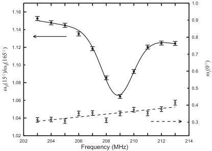
Figure 1: On-line NMR/ON curve for ⁵⁹Cu isotope. Plotted is the ratio of the count rates for two detectors at $15^{\circ}$ and $165^{\circ}$ with respect to the quantization axis as a function of frequency. At the bottom, the count rate at $0^{\circ}$ is shown for the 136 keV $\gamma$ ray of the ${}^{57}\rm{Co}\it{Fe}$ thermometer (corresponding to a sample temperature of about 10 mK) for the same frequency region, showing no effect at the position of the ⁵⁹Cu resonance. The slope in the count rates is caused by a small increase of the sample temperature with the resonance frequency. (arrows indicate the vertical scale that applies; from ref. Golovko04 )

IV.1.1 Demagnetization field

The calculation of the demagnetization field is not straightforward, but for the simple shapes and thin foils (magnetized in the plane of the foil) that were used in the $\beta$-NMR/ON measurements discussed here, analytical expressions can be obtained Chikazumi64 . At the current level of precision, the small demagnetization fields in the foils used, which are of the order of 0.01 T, cannot be neglected.

The foil used by the Leuven group for the measurement with ⁵⁹Cu had a size of 9 mm by 14 mm and an initial thickness of 125 $\mu$m. It was polished with diamond-base paste with grain sizes of 3 $\mu$m and 1 $\mu$m. It is estimated that this reduced the thickness of this foil to (95 $\pm$ 20) $\mu$m. For this a demagnetization field $B_{\rm{dem}}$ = 0.020(4) T is calculated. The foils used by the Oxford group for the measurements with ⁶⁷Cu, ⁶⁹Cu and ⁷¹Cu had an initial thickness of 250 $\mu$m VanEsbroeck05 . They were first polished with sand paper with CAMI (Coated Abrasive Manufacturers Institute) grit designation 600 (i.e. with an average particle diameter of 16 $\mu$m) and thereafter also with diamond-base paste. Due to the larger particle diameter used in the first step, this procedure removed more material from the foils leading to an estimated thickness of (190 $\pm$ 40) $\mu$m. For typical dimensions of 10 mm by 15 mm for such foils, a demagnetization field $B_{\rm{dem}}$ = 0.036(8) T is then calculated for the measurements with ⁶⁷Cu, ⁶⁹Cu and ⁷¹Cu.

IV.1.2 Knight shift

The Knight shift for copper in iron has never been determined at low temperatures. For other elements in ferromagnetic host materials Knight shift values ranging from zero to about 5% have been reported Yazidjoglou1993 . Thus, for the low external fields, $B_{\rm{app}}$, of 0.1 T and 0.2 T that were used in the $\beta$-NMR/ON measurements discussed here, the Knight shift corrections could amount up to about 0.005 T and 0.010 T, respectively. These values were then used as the 1$\sigma$ error bars on the values for the externally applied magnetic fields. Note that the precision to which these external fields could be set is an order of magnitude better and can therefore be neglected at the current level of precision.

IV.2 Results for ⁵⁹Cu, ⁶⁹Cu and ⁷¹Cu

The magnetic moment values and the resonance frequencies for the isotopes ⁵⁹Cu, ⁶⁹Cu and ⁷¹Cu are listed in Table 1 (the case of ⁶⁷Cu will be discussed separately in the next section). Also listed there are the values for the total magnetic field, $B_{\rm{tot}}$, obtained for each isotope using Eq. 1, as well as the hyperfine field, $B_{\rm{hf}}$, that is then obtained from Eq. 2 using the values for the externally applied field, $B_{\rm{app}}$, and the demagnetization field, $B_{\rm{dem}}$.

As can be seen, the hyperfine field values obtained for these three isotopes are in very good agreement with each other (see also Fig. 2). Combining all three results yields a weighted average value of

$$B_{\rm{hf}}({\rm Cu}\it{Fe})~{}=~{}\rm{-21.794(10)~{}T}~{}.$$ (3)

The differences between the hyperfine field values obtained for the three isotopes listed in Table 1 could be due to small differences in the distribution of the nuclear magnetization over the nuclear volume for the three isotopes, i.e. hyperfine anomalies Butgenbach84 . The usual definition for the hyperfine anomaly, $\epsilon_{i}$, for a single nuclear state $i$ is

$$B_{\rm{eff}}=B_{\rm{0}}(1+\epsilon_{i}).$$ (4)

where $B_{\rm{eff}}$ is the hyperfine field averaged over the distribution of nuclear magnetization of the state $i$ and $B_{\rm{0}}$ is the hyperfine field at $r$ = 0. The difference of the hyperfine anomalies of two nuclear states in the same host metal is then given by

$${}^{1}\Delta^{2}=\epsilon_{1}-\epsilon_{2}=\frac{B_{\rm{eff}}^{1}}{B_{\rm{eff}}^{2}}-1.$$ (5)

When considering the possible presence of hyperfine anomalies the values for $B_{\rm{hf}}$ listed in Table 1 have to be interpreted as values for $B_{\rm{eff}}$. It then turns out that the differences of the hyperfine anomalies of these three isotopes are less than 3 $\times$ 10^-3 (see Table 1; 90% C.L.). Note that previously the hyperfine anomaly between ⁶³Cu and ⁶⁵Cu was estimated to be less than 5 $\times$ 10^-5 Locher74 , while in the recent collinear laser spectroscopy measurements on Cu isotopes Vingerhoets10 , no indication for hyperfine anomalies was observed either for the series of isotopes ranging from $A$ = 61 to 75.

For ⁵⁹Cu, two other values for the magnetic moment were recently quoted as well, i.e. $\mu(^{59}$Cu) = 1.83(4) $\mu_{N}$, from in-source laser spectroscopy Stone08b , and $\mu(^{59}$Cu) = 1.910(4) $\mu_{N}$, from an in-gas-cell laser spectroscopy experiment Cocolios09 ; Cocolios10 . As the first value is much less precise than the one obtained from collinear laser spectroscopy it is not further used here. The second value differs well outside error bars from the collinear laser spectroscopy result (see Table 1). Combining it with the $\beta$-NMR/ON resonance frequency of 208.79(4) MHz for ⁵⁹Cu reported in Ref. Golovko04 , a hyperfine field value of $B_{\rm{hf}}(\rm{Cu}\it{Fe}$) = $-$21.59(5) T is obtained. This differs by about 4 standard deviations from the values listed in Table 1 that resulted from combining resonance frequencies and magnetic moment values that were each obtained with the same experimental setups. This difference might be the due to unforeseen systematic effects in this measurement Cocolios09 which was performed with a different experimental setup, as is currently being investigated Cocolios11 .

IV.3 The case of ⁶⁷Cu

The situation for ⁶⁷Cu turns out to be more complicated. In Ref. Rikovska2000b , the magnetic moment of ⁶⁷Cu obtained with the Oxford LTNO setup is given as $\mu(^{67}$Cu) = +2.54(2) $\mu_{N}$; in Ref. Rikovska1999 this result is quoted as $\mu$ = +2.536(3) $\mu_{N}$ (this smaller error bar most probably only reflects the statistical precision). The authors do not quote a resonance frequency value, but analysis of the resonance curve shown in Ref. Rikovska2000b yields a central value of $\nu_{\rm{res}}$ = 278.38(6) MHz. In combination with the magnetic moment value of $\mu$ = +2.536 $\mu_{N}$, this yields a total magnetic field of $-$21.60 T. Comparing this with the hyperfine field value of $-$21.8(1) T for copper in iron that was used in Ref. Rikovska2000b and neglecting the demagnetization field (as the authors of Ref. Rikovska2000b also did), yields a value of +0.20 T for the externally applied magnetic field instead of the value of +0.10 T mentioned in Refs. Rikovska1999 ; Rikovska2000b . The latter value is therefore most probably a typographical error.
When combining the above resonance frequency of 278.38(6) MHz with the magnetic moment value $\mu(^{67}$Cu) = +2.5142(6) $\mu_{N}$ from the laser spectroscopy experiments Vingerhoets10 , a hyperfine field value of $B_{\rm{hf}}(\rm{Cu}\it{Fe})$ = $-$21.952(15) T is obtained for $B_{\rm{ext}}$ = 0.20(1) T and with $B_{\rm{dem}}$ = 0.036(8) T for the foils of the Oxford team (see Sec. IV.1.1). If the demagnetization field is neglected $B_{\rm{hf}}(\rm{Cu}\it{Fe})$ = $-$21.988(15) T is obtained. Both values are at variance with the ones obtained for the other Cu isotopes (see Table 1 and Fig. 2).
Concluding, there seems to be a problem with the $\beta$-NMR/ON result for ⁶⁷Cu that was obtained using another experimental setup than the one used for the isotopes ⁵⁹Cu, ⁶⁹Cu and ⁷¹Cu. The origin of this may e.g. be an undetected error in the frequency calibration. We therefore did not include the $\beta$-NMR/ON result for ⁶⁷Cu in the hyperfine field analysis presented here.

Table 1: Data used for the determination of the hyperfine field of Cu impurities in Fe and values deduced from these. The error bar on the weighted average was increased by a factor $\sqrt{\chi^{2}/\nu}$ = $\sqrt{1.22}$ to account for the fact that the reduced $\chi^{2}$ is larger than unity. The last column lists the hyperfine anomaly differences between ⁶⁹Cu and the two other isotopes.

Isotope	$\mu$	Ref.	$\nu_{\rm{res}}$	Ref.	$B_{\rm{tot}}$	$B_{\rm{app}}$	$B_{\rm{dem}}$	$B_{\rm{hf}}$	${}^{X}\Delta^{69}$
	($\mu_{N}$)		(MHz)		(T)	(T)	(T)	(T)	(%)
59Cu	$+1.8910(9)$	Vingerhoets11	$208.79(4)$	Golovko04	$-21.727(11)$	$0.100(5)$	$0.020(4)$	$-21.807(13)$	0.15(9)
69Cu	$+2.8383(10)$	Vingerhoets10	$311.7(1)$	Rikovska2000b	$-21.611(10)$	$0.20(1)$	$0.036(8)$	$-21.775(16)$	-
71Cu	$+2.2747(8)$	Flanagan09	$250.00(14)$	Stone08a	$-21.627(14)$	$0.20(1)$	$0.036(8)$	$-21.791(19)$	0.07(11)
Weighted average								$-21.794(10)$

Sign from Kontani67 . From the Refs. listed in column 3. Calculated with the formulas derived in Ref. Chikazumi64 (see also Sect. IV.1.1).

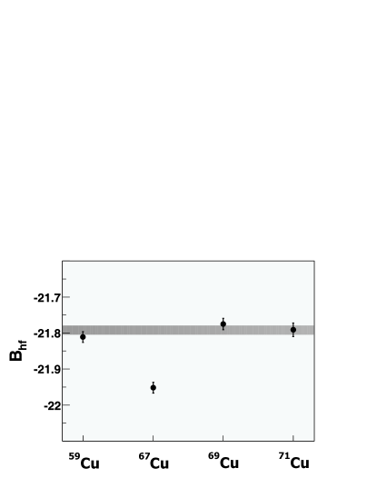
Figure 2: Hyperfine field values (in Tesla) for Cu in Fe obtained by combining resonance frequencies from $\beta$-NMR/ON measurements on the isotopes ⁵⁹Cu, ⁶⁷Cu, ⁶⁹Cu and ⁷¹Cu with the magnetic moments for these isotopes from collinear laser spectroscopy. The grey band indicates the weighted average of the values from ⁵⁹Cu, ⁶⁹Cu and ⁷¹Cu.

Table 2: Overview of hyperfine magnetic fields for Cu in Fe host reported in the literature. Note that in most cases no error bar was quoted.

$B_{\rm{hf}}$ (T)	Ref.	method
$21.0$	Koi62	NMR
$21.77$	Kushida62	NMR
$-21.27$	Shirley65	NMR
$21.79$	Edmonds66	NMR
$-21.3$	Kontani67	spin-echo
$21.8(1)$	Khoi75 ; Rikovska2000a	NMR
$21.3$	Riedi81	NMR
$-21.84$	Kasamatsu86	NMR
$16.95(51)$	Lohmann93	$\gamma-\gamma$ PAC

perturbed angular correlation.

V Previous results

Table 2 lists other values for the hyperfine field of Cu in Fe that are available in the literature, most of which were obtained in classical NMR experiments at room temperature and with - unfortunately - no error being quoted. As can be seen, most values are in reasonable agreement with the new value of $-$21.794(10) T presented here. The value from the $\gamma$-$\gamma$ perturbed angular correlation measurement, which is significantly deviating from all other results, is either wrong or might be related to a different lattice site for Cu impurities in Fe.

VI Comparison with theoretical values

Hyperfine fields in solids can be calculated from first principles. This allows understanding trends in those hyperfine fields as a function of the impurity element in e.g. an iron matrix Akai84 ; Akai85a ; Akai85b ; Korhonen00 ; Cottenier00 ; Torumba06 ; Torumba08 , and it allows disentangling the hyperfine field into contributions with a different physical origin Novak03 ; Torumba06 ; Torumba08 ; Peltzer09 . We have calculated the hyperfine field of Cu in Fe within the framework of Density Functional Theory Kohn64 ; Kohn65 ; DFT-LAPW02 , using the Perdew-Burke-Ernzerhof (PBE) exchange-correlation functional Perdew96 . For solving the scalar-relativistic Kohn-Sham equations we employed the Augmented Plane Waves + local orbitals (APW+lo) method Sjostedt00 ; Madsen01 ; DFT-LAPW02 as implemented in the wien2k package Wien99 for periodic solids. In this method the wave functions are expanded into spherical harmonics inside nonoverlapping atomic spheres of radius $R_{\mathrm{MT}}$ and in plane waves in the remaining space of the unit cell, i.e. the interstitial region. We took $R_{\mathrm{MT}}^{\mathrm{Fe}}=R_{\mathrm{MT}}^{\mathrm{Cu}}=$ 2.30 a.u. . The plane wave expansion of the wave function in the interstitial region was truncated at a large value of $K_{\mathrm{max}}=8.0/R_{\mathrm{MT}}^{\mathrm{min}}=$ 3.48 a.u.^-1, which leads to very accurate values for the calculated hyperfine fields. A dense mesh of k-points, corresponding to a 20$\times$20$\times$20 mesh for a conventional bcc unit cell for Fe, was taken. Spin-orbit coupling was taken into account by a second variational step scheme Koeling77 using a cutoff energy E_SO= 5.0 Ry. The substitutional Cu impurity was modeled by a 128-atom supercell, and all atoms in the supercell were allowed to adjust their positions due to the presence of the impurity. The lattice constant for the Fe-matrix was taken to be the equilibrium lattice constant for the PBE functional (2.8404 $\AA$). These settings allow for an excellent numerical convergence of the hyperfine field.

The results of the calculations are summarized in Table 3.

Table 3: Calculated values for the Fermi contact field, orbital hyperfine field, dipolar hyperfine field and atomic dipolar hyperfine field for a Cu impurity in Fe. Spin and orbital contributions to the atomic magnetic moment for Cu ($\mu_{B}$) and distance between Cu and its first Fe-neighbor ($\AA$).

B(T)
$B_{\rm{F}}$	$-25.32$	$\mu_{\rm{spin}}$	0.115
$B_{\rm{orb}}$	$0.60$	$\mu_{\rm{orb}}$	0.007
$B_{\rm{dip}}$	$-0.01$	$d_{\rm{Cu-Fe}}$	2.478
$B_{\rm{dip}}^{\rm{at}}$	$0.00$

As can be seen, the distance between the Cu impurity and its first eight Fe neighbours is expanded only slightly (0.75 %) compared to the Fe-Fe distance of 2.460 $\AA$ in pure Fe. The dominant contribution to the hyperfine field is the Fermi contact term, caused by s-electron spin polarization, due to the small atomic (d-electron) magnetic moment at the Cu atom. This value can be further split into a core contribution due to 1s and 2s electrons ($-$8.54 T), a semi-core contribution by the 3s-electrons (+5.80 T) and a valence contribution by 4s electrons ($-$22.59 T). The result for the Fermi contact hyperfine field can be compared with the $-$18.2 T that was obtained 25 years ago by the Korringa-Kohn-Rostoker Green’s function method Akai85a . The orbital hyperfine field of Cu (0.60 T) is an order of magnitude smaller than the corresponding quantity in pure Fe, consistent with the very small atomic orbital magnetic moment of Cu. All contributions to the hyperfine field, together with the Lorenz field (0.74 T), sum to a total hyperfine field of $-$23.99 T. Although this is about 2 T larger than the experimental value determined in this work, this deviation is state-of-the-art, and is due to inherent limitations of the chosen exchange-correlation functional.

VII Conclusion

Combining resonance frequencies for the isotopes ⁵⁹Cu, ⁶⁹Cu and ⁷¹Cu obtained from $\beta$-NMR/ON measurements with the NICOLE LTNO setup at ISOLDE, with magnetic moment values obtained for these isotopes in collinear laser spectroscopy measurements at ISOLDE, the hyperfine field of Cu impurities in iron is found to be $B_{\rm{hf}}(\rm{Cu}\it{Fe}$) = $-$21.794(10) T. This value is in agreement with but almost an order of magnitude more precise than the previously adopted value of $-$21.8(1) T and in good agreement with predictions from ab initio calculations. Interpreting the differences between the hyperfine field values obtained for the individual isotopes to be due to hyperfine anomalies, the hyperfine anomalies in Fe for the isotopes considered here were found to be smaller than 3 $\times$ 10^-3 (90% C.L.).

VIII Acknowledgement

This work was supported by the Fund for Scientific Research Flanders (FWO), project GOA/2004/03 of the K. U. Leuven, the Interuniversity Attraction Poles Programme, Belgian State Belgian Science Policy (BriX network P6/23), and the grant LA08015 of the Ministry of Education of the Czech Republic.

References

- (1) G. Rao, Hyperfine Interact. 24-26, 1119 (1985).
- (2) E. Bodenstedt, in The Electromagnetic Interaction in Nuclear Spectroscopy, edited by W.D. Hamilton (North-Holland, Amsterdam, 1975), p. 735.
- (3) G. Goldring and M. Hass, in Treaties on Heavy Ion Science Vol. 3, edited by D. Allan Bromley (Plenum, New York, 1985) 539.
- (4) N. J. Stone in Low-Temperature Nuclear Orientation, editors H. Postma and N. J. Stone (North-Holland, Amsterdam, 1986).
- (5) H. Akai, M. Akai, S. Blügel, R. Zeller, and P.H. Dederichs, J. Phys. Soc. Jpn. 45, 291 (1984).
- (6) M. Akai, H. Akai, and J. Kanamori, J. Phys. Soc. Jpn. 54, 4246 (1985).
- (7) M. Akai, H. Akai, and J. Kanamori, J. Phys. Soc. Jpn. 54, 4257 (1984).
- (8) T. Korhonen, A. Settels, N. Papanikolaou, R. Zeller, and P.H. Dederichs, Phys. Rev. B 62, 452 (2000).
- (9) S. Cottenier and H. Haas, Phys. Rev. B 62, 461 (2000).
- (10) D. Torumba, V. Vanhoof, M. Rots, and S. Cottenier, Phys. Rev. B 74, 014409 (2006).
- (11) D. Torumba, P. Novák, and S. Cottenier, Phys. Rev. B 77, 155101 (2008).
- (12) H. Ebert, R. Zeller, B. Drittler, and P.H. Dederichs, J. Appl. Phys. 67, 4576 (1990).
- (13) N. Severijns et al., Phys. Rev. C 79, 064322 (2009).
- (14) J. Wouters, N. Severijns, D. Vandeplassche, E. van Walle, and L. Vanneste, Phys. Lett. A 124, 377 (1987).
- (15) W. Vanderpoorten, P. De Moor, P. Schuuramns, R. Siebelink, L. Vanneste, J. Wouters, N. Severijns, J. Vanhaverbeke, R. Eder, and H. Haas, Hyperfine Interact. 75, 331 (1992).
- (16) C. J. Ashworth, P. Back, S. Ohya, N. J. Stone and J. P. White, Hyperfine Interact. 59, 461 (1990).
- (17) B. Will et al., Phys. Rev. B 57, 11527 (1998).
- (18) L. Khoi, P. Veillet, and I. Campbell, J. Phys. F 5, 2184 (1975).
- (19) J. Rikovska and N. J. Stone, Hyperfine Interact. 129, 131 (2000).
- (20) M. Kontani and J. Itoh, J. Phys. Soc. Japan 22, 345 (1967).
- (21) H. Akai, M. Akai, and J. Kanamori, J. Phys. Soc. Jpn 54, 4257 (1985).
- (22) V. V. Golovko et al., Phys. Rev. C 70, 014312 (2004).
- (23) J. Rikovska et al., Phys. Rev. Lett. 85, 1392 (2000).
- (24) N. J. Stone et al., Phys. Rev. C 77, 014315 (2008).
- (25) K. T. Flanagan et al., Phys. Rev. Lett. 103, 142501 (2009).
- (26) P. Vingerhoets et al., Phys. Rev. C 82, 064311 (2010).
- (27) P. Vingerhoets, PhD thesis, Kath. University Leuven (2011), and submitted to Phys. Lett. A.
- (28) N.J. Stone, Atomic Data and Nuclear Data Tables 90, 75 (2005).
- (29) D. Vandeplassche, E. van Walle, J. Wouters, N. Severijns and L. Vanneste, Phys. Rev. Lett. 57, 2641 (1986).
- (30) K. S. Krane, Hyperfine Interact. 15/16, 1069 (1983).
- (31) F. Bacon, J. A. Barclay, W. D. Brewer, D. A. Shirley, and J. E. Templeton, Phys. Rev. B 5, 2397 (1972).
- (32) P. Herzog in Ref. Stone86 , p. 953.
- (33) P. D. Johnston, R. A. Fox, and N. J. Stone, J. Phys. C, 5, 2077 (1972).
- (34) E. Hagn, Hyperfine Interact. 22, 19 (1985).
- (35) H. Pattyn et al., Hyp. Int. 2, 362 (1976).
- (36) U. Dämmrich and P. Herzog, Hyperfine Interact. 43, 169 (1988).
- (37) E. van Walle, D. Vandeplassche, J. Wouters, N. Severijns, and L. Vanneste, Phys. Rev. B 34, 2014 (1986).
- (38) W. D. Brewer in Ref. Stone86 , Chap. 9.
- (39) N. Yazidjoglou, W. D. Hutchison, and D. H. Chaplin, J. Phys. Condens. Matter 5, 129 (1993).
- (40) S. Chikazumi, Physics of magnetism, Vol. 1 (J. Wiley and Sons, New York, 1964).
- (41) A. Mueller et al., Nucl. Phys. A 403, 234 (1983).
- (42) H. Franberg et al., Nucl. Instrum. Methods Phys. Res. B 204, 4502 (2008).
- (43) E. Mané et al., Eur. Phys. J. A 42, 503 (2009).
- (44) K. Schlösser, I. Berkes, E. hagn, P. Herzog, T. Niinikoski, H. Postma, C. Richard-Serre, J. Rikovska, N. J. Stone, L. Vanneste, E. Zech and the NICOLE and ISOLDE Collaborations, Hyperfine Interact. 43, 141 (1988).
- (45) K. Van Esbroeck, PhD thesis, Cath. University of Leuven (2005), unpublished.
- (46) S. Büttgenbach, Hyperfine Interact. 20, 1 (1984).
- (47) P. R. Locher, Phys. Rev. B 10, 801 (1974).
- (48) N. J. Stone, U. Köster, J. R. Stone, D. V. Fedorov, V. N.Fedoseyev, K. T. Flanagan, M. Hass, and S. Lakshmi, Phys. Rev. C 77, 067302 (2008).
- (49) T. E. Cocolios et al., Phys. Rev. Lett. 103, 102501 (2009).
- (50) T. E. Cocolios et al., Phys. Rev. C 81, 014314 (2010).
- (51) T. E. Cocolios, private communication (2011).
- (52) J. Rikovska et al., CERN document CERN/ISC 99-6, ISC/P-79 Addendum 1.
- (53) Y. Koi, T. Kushida, T. Hihara, and A. Tsujimura, J. Phys. Soc. Jpn. 17, 96 (1962).
- (54) T. Kushida, A. H. Silver, Y. Koi, and A. Tsujimura, J. Appl. Phys. 33, 1079 (1962).
- (55) D. A. Shirley and G. A. Westenbarger, Phys. Rev. 138, A170 (1965).
- (56) D. Edmonds and G. Wilson, Phys. Lett. 23, 431 (1966).
- (57) M. Kontani and J. Itoh, J. Phys. Soc. Jpn. 22, 345 (1967).
- (58) P. Riedi and G. Webber, J. Phys F 11, 1669 (1981).
- (59) Y. Kasamatsu, T. Hihara, K. Kojima, and T. Kamigaichi, J. Magn. Magn. Mater. 54-57, 1107 (1986).
- (60) E. Lohmann, K. Freitag, T. Schaefer, and R. Vianden, Hyperfine Interact. 77, 103 (1993).
- (61) P. Novák, J. Kuneš, W.E. Pickett, Wei Ku, and F. R. Wagner, Phys. Rev. B 67, 140403(R) (2003).
- (62) E. L. Peltzer y Blancá, J. Desimoni, N. E. Christensen, H. Emmerich, and S. Cottenier, Phys. Status Solidi B 246, 909 (2009).
- (63) P. Hohenberg and W. Kohn, Phys. Rev. 136, B864 (1964).
- (64) W. Kohn and L. J. Sham, Phys. Rev. 140, A1133 (1965).
- (65) S. Cottenier, Density Functional Theory and the Family of (L)APW-methods: a step-by-step introduction, Instituut voor Kern- en Stralingsfysica, KULeuven, Belgium, ISBN 90-807215-1-4 (freely available from http://www.wien2k.at/reg_user/textbooks).
- (66) J. P. Perdew, K. Burke, and M. Ernzerhof, Physical Review Letters 77, 3865 (1996).
- (67) E. Sjöstedt , L. Nordström, and D. J. Singh, Solid State Communications 114, 15 (2000).
- (68) G. K. H. Madsen, P. Blaha, K. Schwarz, E. Sjöstedt, and L. Nordström, Physical Review B 64, 195134 (2001).
- (69) P. Blaha, K. Schwarz, G. Madsen, D. Kvasnicka, and J. Luitz, WIEN2k, An Augmented Plane Wave+Local Orbitals Program for Calculating Crystal Properties (Karlheinz Schwarz, Technische Universit t Wien, Austria, 1999).
- (70) D. D. Koelling and B. N. Harmon, J. Phys. C 10, 3107 (1977).