Maximum relative height of elastic interfaces in random media

Abstract

The distribution of the maximal relative height (MRH) of self-affine one-dimensional elastic interfaces in a random potential is studied. We analyze the ground state configuration at zero driving force, and the critical configuration exactly at the depinning threshold, both for the random-manifold and random-periodic universality classes. These configurations are sampled by exact numerical methods, and their MRH distributions are compared with those with the same roughness exponent and boundary conditions, but produced by independent Fourier modes with normally distributed amplitudes. Using Pickands’ theorem we derive an exact analytical description for the right tail of the latter. After properly rescaling the MRH distributions we find that corrections from the Gaussian independent modes approximation are in general small, as previously found for the average width distribution of depinning configurations. In the large size limit all corrections are finite except for the ground-state in the random-periodic class whose MRH distribution becomes, for periodic boundary conditions, indistinguishable from the Airy distribution. We find that the MRH distributions are, in general, sensitive to changes of boundary conditions.

I Introduction

Recent theoretical progress have highlighted the importance of extreme value statistics (EVS) in statistical physics bouchaud_mezard ; bouchaud_biroli_review . This often yields interesting questions of EVS for strongly correlated variables, a field which, to a large extent, remains to be explored. For homogeneous systems, it has been recently shown that EVS is an interesting tool to characterize the statistics of one-dimensional stochastic processes, like Brownian motion and its variants, which can be mapped onto models of elastic interfaces RCPS ; satya_airyshort ; satya_airylong ; schehr_airy ; GMOR ; RS09 ; RS10 .

Such elastic interfaces are ubiquitous in nature and in the simplest one-dimensional case they can be parameterized by a scalar displacement field $u(x)$, for a system of length $L$. Here we consider periodic boundary conditions (pbc), i.e. $u(x=0)=u(x=L)$ and focus on the displacement, or relative height, $h(x)=u(x)-(1/L)\int_{0}^{L}{\mathrm{d}}x^{\prime}\ u(x^{\prime})$. It can be decomposed into Fourier modes

$$h(x)=\sum_{n=1}^{\infty}a_{n}\cos{\left(\frac{2\pi n}{L}x\right)}+b_{n}\sin{\left(\frac{2\pi n}{L}x\right)}\;,$$ (1)

where $a_{n}$’s and $b_{n}$’s are random variables, whose statistics depend on the precise model under considerations. The geometry of such interfaces (1) is usually characterized by the sample-dependent roughness $w^{2}$ and its ensemble average ${\rm w}_{L}^{2}$ barabasi_stanley ,

$$w^{2}=(1/L)\int_{0}^{L}h(x)^{2}\;,{\rm w}_{L}^{2}=\langle w^{2}\rangle,$$ (2)

where the brackets $\langle...\rangle$ denotes an average over $a_{n}$’s and $b_{n}$’s. Of particular interest are self-affine (or critical) interfaces, characterized by a roughness exponent $\zeta$, such that ${\rm w}_{L}\sim L^{\zeta}$. Relatively recently, the full distribution of $w^{2}$, not only the first moment ${\rm w}^{2}_{L}$, has been considered width_gaussian . It was indeed computed both for Gaussian interfaces, i.e. in the case where $a_{n}$’s and $b_{n}$’s in Eq. (1) are independent Gaussian variables of zero mean and variances $\langle a_{n}^{2}\rangle=\langle b_{n}^{2}\rangle\propto n^{-\alpha}$ [as in Eq. (12) below], corresponding to a roughness exponent $\zeta=(\alpha-1)/2$, for $\alpha>1$ width_gaussian , as well as for pinned interfaces at the depinning threshold width_rosso ; width_frg , where it was studied both numerically and analytically using Functional Renormalization Group (FRG) review_frg . It was subsequently measured for a contact line in a wetting experiment, on a disordered substrate moulinet_width , and also generalized to Gaussian “non-Markovian” ($\alpha\neq 2$) stochastic processes raoul_width . It is interesting to note that such Gaussian interfaces can be physically regarded as an ensemble of free interfaces with non-local harmonic elastic interactions at thermal equilibrium, whose Hamiltonian can be elegantly written in terms of fractional derivatives of order $\alpha/2$ raoul_width ,

$$H[\{h(x)\}]=\frac{1}{2}\int_{0}^{L}{\mathrm{d}}x\;\left[\frac{d^{\alpha/2}h(x)}{dx^{\alpha/2}}\right]^{2}.$$ (3)

Here we focus on the maximal relative height (MRH) $h_{m}$ of such a fluctuating interface (1) defined as

$$h_{m}=\max_{0\leq x\leq L}h(x)\;.$$ (4)

This observable was first introduced and studied numerically for Gaussian interfaces with short range elasticity, such that $\langle a_{n}^{2}\rangle=\langle b_{n}^{2}\rangle\propto n^{-2}$ RCPS , i.e. $\zeta=1/2$, and it was found that $\langle h_{m}\rangle\sim L^{\zeta}$. Then, Majumdar and Comtet obtained an exact analytical expression for the full probability distribution function (pdf) $P(h_{m}|L)$ of $h_{m}$ and showed that it is given by the so-called Airy distribution $f_{\rm Airy}$  satya_airyshort ; satya_airylong ,

$$P(h_{m}|L)=\frac{1}{L^{1/2}}\,f_{\rm Airy}\left(\frac{h_{m}}{L^{1/2}}\right)\;,$$ (5)

where $f_{\rm Airy}$ describes the distribution of the area under a Brownian excursion on the unit time interval. We remind that a Brownian excursion is a Brownian motion conditioned to start and end in $0$ while staying positive in the time interval $[0,1]$.

Incidentally, the same Airy distribution appears also in various, a priori unrelated problems, in graph theory and in computer science majumdar_review . This result (5) was then extended to a wide class of one-dimensional solid-on-solid models schehr_airy , showing the universality of the Airy distribution (5) for interface models with short range elasticity (and without disorder). The distribution of $h_{m}$ was then investigated for Gaussian interfaces with $\alpha>1$ in Ref. GMOR . There it was shown that the distribution has a scaling form similar to Eq. (5), the scaling variable being $h_{m}/L^{\zeta}$, with $\zeta=(\alpha-1)/2$, and where the scaling function depends continuously on the parameter $\alpha$.

A natural, and very physical, extension of these works concerns the maximal height of elastic interfaces in random media: this is the aim of the present paper. In the continuum limit the simplest elastic interface model is described by the Hamiltonian

$$H[\{u(x)\}]=\int_{0}^{L}{\mathrm{d}}x\left\{\frac{c}{2}\left(\nabla u(x)\right)^{2}+V(x,u(x))-fu(x)\right\},$$ (6)

together with an overdamped equation of motion $\partial_{t}u(x,t)\propto-\delta H[\{u(y)\}]/\delta u(x)$. The first term in (6) is the usual harmonic elastic energy, where $c$ is the elastic constant, and tends to straighten the displacement field. The second term is a random potential $V(x,u)$ that models randomly distributed defects both in the direction $x$ along the line and in the direction $u$ along the displacements (see Fig. 1 for a discretized version of this interface to be considered below). The third term represents the action of an external uniform field with strength $f$ that tends to drive the interface in direction $u$. Here we consider a random potential which is a Gaussian random variable with zero mean $\overline{V(x,u)}=0$ and correlations

$$\overline{V(x,u)V(x^{\prime},u^{\prime})}=\delta(x-x^{\prime})R_{0}(u-u^{\prime})\;,$$ (7)

where $\overline{\dots}$ means an average over realizations of disorder with correlator $R_{0}(u)$. We will consider two types of disorder which correspond to two distinct universality classes: the so-called random-manifold (RM) class, and the random-periodic (RP) class. In the RM class $R_{0}(u)$, the bare disorder correlator, is a rapidly decaying function over distances larger than a short-distance cutoff $a$. In the RP class, the disorder has periodic correlations in the $u$ direction, with a given periodicity $a_{0}$, such that $R_{0}(u+na_{0})=R_{0}(u)$ with $n$ an integer. For a given realization of the disorder the steady-state statistics of such interfaces is for $f=0$ described by a Boltzmann weight $\propto\exp{[-\beta H]}$, with $\beta=T^{-1}$ the inverse temperature. For $f\neq 0$ and finite $T$ the system reaches a non-equilibrium moving steady-state at large enough times, while at $T=0$ it can reach a moving steady-state only if the driving force is large enough to overcome the barriers between the disorder-induced metastable states.

Such disordered elastic systems (6) have been widely studied during the last twenty years, in particular because they have found many experimental realizations, ranging from domain walls in ferromagnets domain_walls , contact lines in wetting moulinet_width ; wetting and fracture experiments fracture . They are also relevant to describe periodic structures like charge density waves cdw or vortex lattices in type II superconductors blatter ; giamarchi . In these systems, the competition between elasticity and disorder leads not only to non-trivial ground state configurations but also affects in a dramatic way their dynamical properties. In particular, when driven by an external force $f$ at zero temperature, disorder leads to a depinning transition at a threshold value $f=f_{c}$, below which the interface is immobile, and above which steady-state motion sets in. At finite but small $T$, an ultra-slow steady-state creep motion sets in below $f_{c}$, and in particular, at $f=0$, the zero velocity steady-state coincides with the equilibrium ground-state configuration when $T\to 0$. Interestingly this model (6) has a universal roughness diagram phasediagram described by the crossovers between three types of self-affine interfaces, or “reference steady-states”, depending on the amplitude of the driving force $f$:

• at equilibrium ($f=0$) and $T=0$, which corresponds to the directed polymer in a random medium, where the exponent $\zeta=2/3$ for the RM class kardar , and $\zeta=1/2$ in the RP class rmtorp ; solidonsolid ,

• exactly at the depinning threshold $f=f_{c}$ and $T=0$ where $\zeta\simeq 1.25$ in the RM class rosso_1.25 and $\zeta=3/2$ in the RP class review_frg ; rmtorp ; rmtorp2 ,

• in the limit $f\gg f_{c}$ where, in the moving frame, disorder induced fluctuations of the interface become an effective annealed noise: for the RM class this noise is thermal-like chauve ; phasediagram , yielding the Edwards-Wilkinson roughness $\zeta=1/2$ corresponding to the thermal equilibrium of the system described by Eq. (6) with $V(x,u)=0$, while in the RP class it is a “washboard” colored noise yielding a larger exponent $\zeta=1.5$, identical to the one of the RP depinning rmtorp ; rmtorp2 .

The third case (iii) effectively describes situations with annealed noise rather than quenched noise and in particular, for the RM class, the MRH distribution is simply given by the Airy distribution (5). In the two first cases (i) and (ii) sample to sample fluctuations are important and one expects different fluctuations of the MRH than those produced by annealed noise. It is the purpose of this paper to study the MRH distributions in the two first cases (i) and (ii) above, that we will denote by RMG, RPG for the random-bond (which we also call random-manifold) and random-periodic ground states, and RMD, RPD for the random-bond and random-periodic depinning configurations, respectively. These distributions are thus generated by sample to sample fluctuations of the MRH, while the ensemble of Gaussian signals  (1) can be physically thought as determined by the Boltzmann weight associated to (3) with $T=1$.

We show that, in all the situations considered here, the distribution of the MRH is very well described by the one corresponding to a Gaussian interface, where $a_{n}$’s and $b_{n}$’s in Eq. (1) are independent Gaussian variables [as in Eq. (12) below] of zero mean and variances $\langle a_{n}^{2}\rangle=\langle b_{n}^{2}\rangle\propto n^{-(1+2\zeta)}$. Despite of this, our numerical data show some numerical evidence that these distributions are different for the depinning configurations, and also for the ground-states in the random-manifold class. Note that similar results were obtained for the width distribution at the depinning threshold width_rosso , which were further justified using FRG calculations width_frg . In that case, using FRG close to the upper critical dimension, in dimension $d=4-\epsilon$, it was shown that the displacement field can be written as $u=\sqrt{\epsilon}u_{0}+\epsilon u_{1}$ where $u_{0}$ is a Gaussian random variable of order ${\cal O}(1)$ while $u_{1}$ is a random variable with non-Gaussian fluctuations, also of order ${\cal O}(1)$ width_frg . Motivated by these similarities with the Gaussian interface, we revisit the analysis of the right tail of the pdf of the MRH for Gaussian interfaces and generic $\zeta$ where we obtain exact results, using Pickands’ theorem pickands . For the ground-states in the random-periodic class with periodic boundary conditions we find that corrections to the Gaussian independent modes approximation vanish at large system sizes and thus the MRH distribution becomes indistinguishible from the universal Airy distribution. Finally, for the equilibrium case we show that the MRH distribution is sensitive to the boundary conditions, highlighting their importance in the study of anomalous, self-affine interfaces.

The paper is organized as follows: in Section II, we remind the results that were obtained for Gaussian interfaces, and derive the precise asymptotic behavior of the right tail of the distribution of the MRH. In Section III, we provide the details of our numerical simulations, the results of which are then presented in Section IV. In Section V, we discuss these results before we conclude in Section VI. Some details relative to the use of Pickand’s theorem have been left in appendix A.

II Results for Gaussian interfaces

We first start to remind the known results for Gaussian interfaces, without disorder. The distribution of $h_{m}$ was first studied for the simplest model of an elastic interface described by Eq. (6) with $V=0$, $f=0$ and periodic boundary conditions, i.e. $u_{L}=u_{0}$. In that case one has ${\rm w}_{L}^{2}=TL/12$. While a first numerical study indicated that $h_{m}\sim L^{\zeta}$, with $\zeta=1/2$, Majumdar and Comtet were then able to compute exactly the full distribution of $h_{m}$ satya_airyshort ; satya_airylong , $P(h_{m}|L)=\frac{1}{L^{1/2}}\,f_{\rm Airy}\left(\frac{h_{m}}{L^{1/2}}\right)$ where $f_{\rm Airy}$ is the so-called Airy distribution, whose Laplace transform is given by

$$\int_{0}^{\infty}f_{\rm Airy}(x)e^{-sx}dx=s\sqrt{2\pi}\sum_{k=1}^{\infty}e^{-\alpha_{k}s^{2/3}2^{-1/3}},$$ (8)

where $\alpha_{k}$’s are the amplitudes of the zeros of the Airy function on the negative real axis. For instance, $\alpha_{1}=2.3381\dots$, $\alpha_{2}=4.0879\dots$, $\alpha_{3}=5.5205\dots$ etc abramowitz . It is also possible to invert this Laplace transform to obtain satya_airyshort ; satya_airylong ; takacs_invert

$$f_{\rm Airy}(x)=\frac{2\sqrt{6}}{x^{10/3}}\sum_{n=1}^{\infty}e^{-b_{n}/x^{2}}b_{n}^{2/3}U(-5/6,4/3,b_{n}/x^{2})\;,$$ (9)

where $b_{n}=2\alpha_{n}^{3}/27$ and $U(a,b,z)$ is the confluent hypergeometric (Tricomi’s) function abramowitz . Its asymptotic behavior is given, for small argument by

$$f_{\rm Airy}(x) \sim \frac{8}{81}\alpha_{1}^{9/2}x^{-5}\,e^{-2\alpha_{1}^{3}/{27x^{2}}}\quad{\rm for}\quad x\to 0\;.$$ (10)

The large argument behavior was obtained in Refs. satya_airylong ; janson_louchard

$$f_{\rm Airy}(x)\sim{72}{\sqrt{\frac{6}{\pi}}}x^{2}e^{-6x^{2}}\quad{\rm for}\quad x\to\infty\;.$$ (11)

In the above expression, the leading Gaussian behavior, $e^{-6x^{2}}$, was obtained in Ref. satya_airylong while the subleading prefactor, ${72}{\sqrt{\frac{6}{\pi}}}x^{2}$ was obtained in Ref. janson_louchard using rather involved combinatorial techniques [which also allow to obtain the subleading corrections to (11)]. We show below that this result (11) can be straightforwardly obtained using Pickands’ theorem pickands concerning the asymptotic properties of the maximum of a stationary Gaussian (see also appendix A for more details).

The MRH distribution was then investigated for Gaussian interfaces displaying a $1/f^{\alpha}$ power spectrum in Ref. GMOR . Considering again periodic boundary conditions, $h(0)=h(L)$, the relative height field can be written in a Fourier expansion as in Eq. (1) with a Gaussian probability measure:

$${\cal P}[h]\propto\exp\left[-\frac{1}{4}\sum_{n=1}^{\infty}\frac{(2\pi n)^{\alpha}}{L^{\alpha-1}}(a_{n}^{2}+b_{n}^{2})\right]\;,$$ (12)

corresponding to independent Gaussian random variables $a_{n}$’s and $b_{n}$’s of zero mean and variance, for $n\geq 1$

$$\langle a_{n}a_{n^{\prime}}\rangle=\langle b_{n}b_{n^{\prime}}\rangle=\delta_{n,n^{\prime}}\frac{2L^{\alpha-1}}{(2\pi n)^{\alpha}}\;,$$ (13)

while $\langle a_{n}b_{n^{\prime}}\rangle=0$. Note that this is the same convention as the one chosen in Ref. GMOR , which yields in particular

$${\rm w}^{2}_{L}=\frac{2L^{\alpha-1}}{(2\pi)^{\alpha}}{\bm{\zeta}}(\alpha)\;,\;{\bm{\zeta}}(\alpha)=\sum_{n=1}^{\infty}n^{-\alpha}\;,$$ (14)

where ${\bm{\zeta}}(\alpha)$ is the Riemann zeta function. The roughness exponent is thus $\zeta=(\alpha-1)/2$. In Ref. GMOR it was shown that the distribution of the MRH takes the scaling form

$$P(h_{m}|L)=\frac{1}{L^{\zeta}}\tilde{f}_{\alpha}\left(\frac{h_{m}}{L^{\zeta}}\right)\;,$$ (15)

where from now on, the tilde over any distribution function indicates that it corresponds to Gaussian interfaces described by Eq. (12). While the exact expression of the scaling function $\tilde{f}_{\alpha}(x)$ is known only for $\alpha=2$, see Eqs. (5, 9). Nevertheless, for $\alpha=2n$ where $n\in\mathbb{N}$, the computation of the $P(h_{m}|L)$ can be formulated in terms of a path integral GMOR from which several properties can be deduced. In particular, the small argument behavior of the scaling function can be studied in detail, yielding GMOR

$$\tilde{f}_{\alpha}(x)\sim Cx^{-\gamma}\exp{(-B/x^{\beta})}\;,$$ (16)

with

$$\beta=\frac{2}{\alpha-1}=\frac{1}{\zeta}\;,\;\gamma=\frac{2\alpha+1}{\alpha-1}=\frac{3+4\zeta}{2\zeta}\;,$$ (17)

while the amplitudes $B$ and $C$ can be expressed in terms of the smallest eigenvalue $\epsilon_{0}\equiv\epsilon_{0}(\alpha)>0$ of a linear eigenvalue problem GMOR :

$$B=\frac{\alpha-1}{2}\left(\frac{2\epsilon_{0}}{\alpha+1}\right)^{\frac{\alpha+1}{\alpha-1}}\;,\;\sqrt{\frac{\alpha+1}{\alpha-1}}\left(\frac{2\epsilon_{0}}{\alpha+1}\right)^{\frac{3}{2}\frac{\alpha+1}{\alpha-1}}\;.$$ (18)

Note that $\epsilon_{0}(2)=\alpha_{1}/2^{1/3}$ so that these formulas (16, 17, 18) coincide with the small argument behavior of the Airy function for $\alpha=2$ (10). While this behavior (16) where the exponents are given by Eq. (17), was shown to hold for $\alpha=2n$, numerical simulations demonstrated its validity for any $\alpha>1$ GMOR . We also notice that the value of this eigenvalue $\epsilon_{0}(\alpha=4)$, corresponding to the Random Acceleration Process, was shown to appear in a completely different problem of random convex geometry, called the Sylvester’s question hilhorst_sylvester .

The large argument behavior of the scaling function $\tilde{f}_{\alpha}(x)$ (15) is harder to treat analytically. Numerical simulations performed in Ref. GMOR showed evidence for the asymptotic behavior:

$$\tilde{f}_{\alpha}(x)\sim Dx^{\delta}e^{-Ex^{2}}\;.$$ (19)

As explained in the Appendix A, we are able to compute this exponent $\delta$ as well as the amplitudes $D$ and $E$ using Pickands’ theorem. One obtains that the exponent $\delta$ depends on $\alpha$ as follows

$$\delta=\begin{cases}&\frac{2}{\alpha-1}\;,1<\alpha<3\\ &1\;,\alpha>3\;,\end{cases}$$ (20)

while one expects logarithmic corrections for $\alpha=3$,which thus appears as a threshold value. These values are consistent with the numerical estimations reported in Ref. GMOR . They are also consistent with the exact result obtained in the limit $\alpha\to\infty$, for which $\delta=1$ GMOR . The amplitude $E$ is given by

$$E=\frac{(2\pi)^{\alpha}}{4{\bm{\zeta}}(\alpha)}\;,$$ (21)

while the amplitude $D$ can be expressed in terms of a Pickands’ constant (A), and has in general a complicated expression. However for $\alpha=2$ and $\alpha>3$ it can be computed explicitly as

$$D=\begin{cases}&72\sqrt{\frac{6}{\pi}}\;,\;{\rm if}\;\alpha=2\;,\\ &\sqrt{\frac{{\bm{\zeta}}(\alpha-2)}{{\bm{\zeta}}(\alpha)}}\frac{(2\pi)^{\alpha}}{2{\bm{\zeta}}(\alpha)}\;,\alpha>3\;.\end{cases}$$ (22)

The expression of $D$ for generic $1<\alpha<3$ is left in Eq. (54) in Appendix A. It is straightforward to check that the results in Eqs. (19, 20, 21, 22) yield back, for $\alpha=2$, the result for the Airy distribution (11).

III Various situations for elastic interfaces in disordered media : details of simulations

We now describe the various models of elastic interfaces that we study using numerical simulations. Numerically, it is very convenient to discretize the internal $x$ direction of the elastic strings described by Eq. (6). Indeed, once conveniently discretized, the ground-states and critical states at depinning can be obtained by exact and fast numerical algorithms. As discussed below, for depinning we can keep $u(x)$ as a continuous variable. For the ground-state it is convenient to also discretize $u(x)$ and work on a lattice. None of these practical choices change the universality classes we analyze, and at large enough $L$ the numerical results for the lattice model should be indistinguishable from those of a continuum model.

III.1 The ground state

When the external force is zero and the finite size pinned interface is allowed to equilibrate at zero temperature it reaches the ground state configuration, found by minimizing the energy (6) for a given sample of disorder. Finding such a state for each disorder realization poses a global optimization problem which can be solved by an exact transfer-matrix method. This method allows to find the ground-state of a line on a lattice where both $u(x)$ and $x$ are discrete variables. For simplicity we impose a hard constraint on the local allowed elongations, $|u(x+1)-u(x)|\leq 1$. This simplification does not change the equilibrium universality class which is thus only determined by the disorder correlator. This is at variance with depinning configurations, where such constraints, or more general non-linear corrections to the standard harmonic elasticity, can change the depinning universality classes rosso_algorithm ; phasediagram . We thus simulate the directed polymer in a random medium as a simple model for the continuum interfaces described by (6), with the universality classes determined by the nature of the discretized disorder potential correlations.

We work on a finite discrete space: we use a rectangular lattice of size $L\times\ell$. Points of the lattice are indexed by the couple of integers $(i,j)$ in the ranges $0\leq i\leq L$ and $0\leq j\leq\ell$. The disordered potential is now a random variable $V_{ij}$ given at each point $(i,j)$ of the described lattice, with zero mean

$$\overline{V_{ij}}=0,$$ (23a)

and correlations

$$\overline{V_{ij}V_{kl}}=\delta_{ik}\delta_{jl}\;.$$ (23b)

In our simulations, we choose Gaussian random variables, although the precise distribution should not be relevant, provided that it remains narrow. We work with periodic boundary conditions both in the $u$ and in the $x$ direction: the sites $(0,j)$ are identified with the sites $(L,j)$, for all $0\leq j\leq\ell$, and in the $u$ direction as well: $(i,0)\equiv(i,\ell)$, for all $0\leq i\leq L$.

Figure 1: The plain blue line represent a path on the lattice when starting in $j_{0}=3$. The pointed maximum is reached at $i=4$ and its value is $j_{4}=6$. If $(j_{i})_{0\leq i\leq L}$ is the sequence of heights visited by the path, one must substract the spatial average $\langle u\rangle=\sum_{i}j_{i}/L$ to obtain the MRH of this sample.

A path $\mathcal{C}$ of length $L$ is given by the sequence of visited sites $(i,j)$, for $0\leq i\leq L-1$, and due to periodic boundary conditions, it can be regarded as a close path on a torus. Its energy is the sum of disordered energies at each visited site:

$$E(\mathcal{C})=\sum_{(i,j)\in\mathcal{C}}V_{ij}\;.$$ (24)

At each step, the path can go from $(i,j)$ to one of the three possibilities $(i+1,j-1)$, $(i+1,j)$ or $(i+1,j+1)$: we then select the optimal path amongst the ensemble $\mathcal{C}_{j_{0}}$ of paths starting in $(0,j_{0})$ and ending in $(L,j_{0})\equiv(0,j_{0})$ by a recursive method kardar . Calling $\mathcal{C}^{*}_{j_{0}}$ this path, one has

$$E_{\text{opt}}(j_{0})=E(\mathcal{C}^{*}_{j_{0}})=\min_{\mathcal{C}_{j_{0}}}E(\mathcal{C}_{j_{0}})\;,$$ (25)

the energy for the optimum path, minimizing the total energy for a fixed starting point $j_{0}$. However considering only these paths $\mathcal{C}^{*}_{j_{0}}$, even averaging over the disorder, yields a non-stationary two-point correlation function of the displacement field. One obtains a stationary correlation function by considering the optimal path $\mathcal{C}^{*}$ among all closed paths on the torus. Then

$$E_{GS}=\min_{\mathcal{C}}E(\mathcal{C})=E(\mathcal{C}^{*}).$$ (26)

From our ensemble of paths $\mathcal{C}^{*}_{j_{0}}$, one has to minimize by varying the starting point $j_{0}$ on the $u$ axis:

$$E_{\textrm{GS}}=\min_{0\leq j_{0}\leq\ell}E_{\textrm{opt}}(j_{0}),$$ (27)

Recalling that $L$ and $\ell$ are the lengths of the disordered substrate in the $x$ and $u$ directions respectively, one has to choose $\ell\gtrsim L^{\zeta_{\textrm{GS}}}$ in order to explore a region of correlated paths. In this case, $\zeta_{\textrm{GS}}$ stands for the ground state roughness exponent, which can take the values $\zeta_{\tt RMG}=2/3$ kardar for the random-mainfold ground state and $\zeta_{\tt RPG}=1/2$ for the random-periodic ground state, respectively. In our simulations, we have taken $\ell=L$ to produce ground states in the RM universality class, while we took $\ell\ll L$, for ground states in the RP universality class. The last choice is equivalent to construct a quenched potential with periodic correlations in the direction of $u$ with period $\ell$. In particular, if we take $\ell\ll L$ but still large compared to the unity, $\ell$ controls the crossover between the RM and RP universality classes, from $\zeta_{\tt RMG}$ to $\zeta_{\tt RPG}$. For this reason, in most of our simulations for the RP class, we set $l\sim O(1)$, thus minimizing the crossover or finite-size effect.

We have produced a number of $10^{6}$ samples of each lengths $L=128,256,512,1024,2048,4096$ in order to construct the histograms of the maximal relative height $h_{m}$. The results we obtain for the MRH and discuss in the next section are computed from stationary paths $\mathcal{C}^{*}$, and are referred with the index RMG, RPG for the random manifold and random periodic universality classes. We discuss the results for the ensemble given by $\mathcal{C}^{*}_{j_{0}}$ (with the arbitrary choice $j_{0}=0$) having a non-stationary correlation function in the section IV.4, for the random-manifold case using the index RMG’ to distinguish from its stationary counterpart RMG. Both cases, RMG and RMG’, have the same roughness exponent $\zeta_{\tt RMG}=\zeta_{\tt RMG^{\prime}}=2/3$.

III.2 The depinning transition

The critical configuration $u_{c}(x)$ of an elastic interface at the depinning transition is an extreme solution of the overdamped equation of motion

$$\frac{\partial u(x,t)}{\partial t}=-\frac{\delta H[\{u(x)\}]}{\delta u(x)}+f=0,$$ (28)

such that $u=u_{c}$ for the largest possible force $f=f_{c}$ satisfying the above equation, with $f_{c}$ the so-called critical force. Above $f_{c}$, the sum of all forces in the second term of Eq. (28) is always positive, and thus a zero velocity steady-state solution can not exist. Middleton’s theorems rosso_1.25 assure that such a solution exists and it is unique. In order to solve numerically Eq. (28) for a given realization of the random potential we can discretize the string in the direction $x$ into $L$ pieces, thus converting Eq. (28) into an inversion problem. Solving the resulting $L$-dimensional system of Eq. (28) for large $L$ by standard general methods is however a formidable task, due to the non-linearity of the pinning force. On the other hand, solving the long-time steady-state dynamics at different driving forces $f$ both below and above $f_{c}$ is very inefficient due to the critical slowing down near $f_{c}$. Fortunately, this problem has a particular analytical structure that allows to devise a precise and very efficient algorithm allowing to obtain iteratively the critical force $f_{c}$ and the critical configuration $u_{c}(x)$ for each independent disorder realization without solving the actual dynamics nor directly inverting the discretized version of Eq. (28)  rosso_algorithm ; rosso_1.25 . In this paper we use such method with periodic boundary conditions in all directions. This guarantees that the critical configurations have spatially stationary correlation functions.

We implement the algorithm to find the critical configuration in 1+1 dimensions as in Ref. rosso_1.25 . We discretize the space in the $x$ direction while keeping $u$ as a continuous variable. A potential $V(x,u)$ satisfying (7) is modeled with random cubic splines. We consider periodic boundary conditions in both directions, in a system of size $L\times\ell$. When $\ell$ is large enough, the critical configuration sample averaged width is well described by ${\rm w}_{L}\equiv[\overline{{u_{c}}^{2}-\overline{u_{c}}^{2}}]^{1/2}\sim L^{\zeta}$ with $\zeta\equiv\zeta_{\tt RMD}\approx 1.25$ rosso_1.25 the random-manifold depinning roughness exponent. We will denote this Random-Manifold depinning case as RMD. For small $\ell$ the average width is well described by the random-periodic depinning roughness exponent $\zeta\equiv\zeta_{\tt RPD}\approx 1.5$ review_frg ; rmtorp ; rmtorp2 . Accordingly, we will denote this Random-Manifold depinning case as RPD. More precisely, for this system it was found that ${\rm w}_{L}\sim G(\ell/L^{\zeta_{\tt RMD}})L^{\zeta_{\tt RMD}}$ for all values of $\ell$ with $G(x)$ a non-monotonic function of $x$, such that $G(x)\sim x^{(1-\zeta_{\tt RPD}/\zeta_{\tt RMD})}$ for $x\ll 1$ and a with a very slow, approximately logarithmic, growth for $x\gg 1$ rmtorp2 . Changing the transverse periodicity thus allows to crossover from the random-manifold to the random-periodic universality class. By using this method we can sample critical configurations belonging to these two classes, RMD and RPD, respectively, and tune the non-universal prefactors ${\rm w}_{L}/L^{\zeta_{\tt RMD}}$, ${\rm w}_{L}/L^{\zeta_{\tt RPD}}$ to different values. Once the critical configuration $u_{c}(x)$ is obtained for each case, we substract the center of mass position $h(x)=u_{c}(x)-(1/L)\int_{0}^{L}dx^{\prime}\;u_{c}(x^{\prime})$ and calculate the MRH from Eq. (4). Repeating this procedure for different disorder realizations gives access to the MRH probability distribution. In our simulations we use between $10^{4}$ and $10^{5}$ critical samples of sizes $L=128,256,512$.

IV Numerical results

We present numerical results of the probability distribution function $P_{k}(h_{m}|L)$ of the maximal relative height $h_{m}$ where the subindex $k={\tt RMG,RPG,RMD,RPD}$ denotes the different cases: random-manifold and random-periodic ground states, and random-manifold and random-periodic critical configurations, respectively.

IV.1 Scaling of $h_{m}$ with $L$

Figure 2: For the random-manifold and random-periodic ground states, $k={\tt RMG,RPG}$, and critical configurations $k={\tt RMD,RPD}$, we plot the rescaled distributions $f_{k}(z)=L^{\zeta_{k}}P_{k}(z\times L^{\zeta_{k}}|L)$, obtained from the histograms $P_{k}(h_{m}|L)$ computed for different system size $L$ as indicated in the key.

For all cases, our numerical data are compatible with the scaling law

$$P_{k}(h_{m}|L)=\frac{1}{L^{\zeta_{k}}}\ f_{k}\left(\frac{h_{m}}{L^{\zeta_{k}}}\right),$$ (29)

where $\zeta_{k}$ is the roughness exponent of the case $k$, $\zeta_{\tt RMG}=2/3$, $\zeta_{\tt RPG}=1/2$, $\zeta_{\tt RMD}\approx 1.25$, and $\zeta_{\tt RPD}=3/2$. In the continuum limit $L\gg 1$, the rescaled functions $f_{k}$ are expected to depend only on the rescaled maximal relative height $z=h_{m}/L^{\zeta_{k}}$. In Fig. 2 one observes that the rescaled distributions for different $L$ of the case $k$ indeed collapse for different sizes of the same class, strongly supporting this scaling relation (29). The different cases, RPG, RMG, RMD and RPD in order of roughness exponent, have very different scaling functions $f_{k}$ in this $L^{\zeta}$ scaling. In particular, it is clearly visible that the most probable value, the mean and also the standard deviation of each $f_{k}$ decreases when the roughness exponent increases. Besides these facts, the curves are somewhat similar, and we are interested in testing other simple scaling forms to compare these distributions $P_{k}(h_{m}|L)$ on the same footing.

IV.2 Average and sigma scaling

Figure 3: For each case $k={\tt RPG,RMG,RMD,RPD}$ we show the average-rescaled distributions $\phi_{k}(x)=\overline{h_{m}}P_{k}(x\overline{h_{m}}|L)$. Different system lengths are shown, as quoted in the key, and the rescaled functions collapse onto the same curves, having unit average.

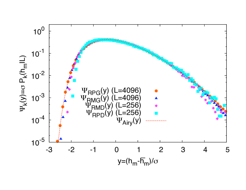
Figure 4: For each case $k={\tt RPG,RMG,RMD,RPD}$ we show the sigma rescaled distributions $\psi_{k}(y)=\sigma P_{k}(\overline{h_{m}}+\sigma y|L)$, obtained with $L=256$ for the depinning cases and $L=4096$ for the ground state cases. Other curves for different $L$ collapse on theses ones and are not shown for clarity. The Airy distribution is shown also with sigma scaling.

Two other scaling forms have been used in the literature GMOR ; width_rosso , namely the average-scaling and the sigma-scaling. The average scaling is defined by

$$P_{k}(h_{m}|L)=\frac{1}{\overline{h_{m}}}\ \phi_{k}\left(\frac{h_{m}}{\overline{h_{m}}}\right),$$ (30)

where the average is computed as

$$\overline{h_{m}}=\int_{0}^{\infty}{\mathrm{d}}h_{m}\,h_{m}\ P_{k}(h_{m}|L).$$ (31)

The rescaled variable $x=h_{m}/\overline{h_{m}}$ has by definition a unit mean. It differs from the precedent scaling by the non-universal prefactor $A_{k}$ in $\overline{h_{m}}=A_{k}L^{\zeta_{k}}$. This prefactor can be indeed physically relevant if there exists a crossover to the asymptotic roughness regime which characterizes the universality class. In such cases, if the crossover to the asymptotic regime takes place at a characteristic length $L_{\times}$, we can expect $\overline{h_{m}}\approx A_{\times}(L/L_{\times})^{\zeta_{k}}$, with $A_{\times}\sim\overline{h_{m}(L_{\times})}$ a characteristic maximal height for a system of size $L_{\times}$. We thus obtain $A_{k}\approx A_{\times}/L_{\times}^{\zeta_{k}}$. Such crossovers usually can depend on microscopic details, such as the strength of the disorder and the elasticity (e.g. the Larkin length), temperature or the spatial discretization when the interface is defined on a lattice. In the case of moving interfaces such crossovers can in addition depend on the velocity phasediagram . As a peculiar case, in very elongated samples the prefactor $A_{k}$ could also depend on the transverse dimension of the system if the configuration carries with it an extreme value over the sample, such as the depinning threshold for the critical configuration rmtorp2 . We present this average scaling in Fig. 3. We see again a very good collapse for the different system sizes within each case $k$, and also observe that the scaling functions $\phi_{k}$ look still very different because the width of the rescaled distributions $\phi_{k}$ appreciably increases when the roughness exponent increases.

Yet another way to present the data is the sigma-scaling defined by

$$P_{k}(h_{m}|L)=\frac{1}{\sigma}\,\psi_{k}\left(\frac{h_{m}-\overline{h_{m}}}{\sigma}\right),$$ (32)

where the standard deviation $\sigma$ is obtained when averaging over the disorder

$$\sigma^{2}=\overline{\left(h_{m}-\overline{h_{m}}\right)^{2}}.$$ (33)

The rescaled variable $y=(h_{m}-\overline{h_{m}})/\sigma$ has zero average and unit standard deviation. This is the most general linear transformation that can get rid of model dependent amplitudes, such as the aforementioned $A_{k}$. It allows then to compare the shape of the distributions on the same footing. Actually, the differences between the distributions $\psi_{k}$ are minute, and not visible on a plot with linear axis. In Fig. 4 we show the sigma-rescaled distributions $\psi_{k}$ obtained from samples with $L=4096$ and $L=256$ for ground states and depinning respectively, using log-linear axis (distributions obtained from other system sizes collapse on the same curves and are not shown for clarity). One can observe that the $\psi_{k}$’s are eventually different: this is especially visible in the left tail. It indicates that the rescaled distributions remain sensitive to the roughness exponent $\zeta$. The Airy distribution function (also plotted in sigma scaling) seems to collapse very well with the RPG case (see the discussion in paragraph IV.3 below). Moreover it gives an approximate description of the remaining cases RMG, RMD, RPD, furnishing an idea of the small and large argument behaviors. In particular we have checked that the large argument behavior of $\psi_{k}(y)$, for each case $k={\tt RPG,RMG,RMD,RPD}$, is well fitted by a Gaussian tail, $\psi_{k}(y)\propto\exp(-d_{k}y^{2})$, although a precise determination of the coefficients $d_{k}$ remains a hard task numerically. Considering this observation together with our exact analytical results for Gaussian interfaces obtained above (19), we conjecture that $\psi_{k}(y)\propto\exp(-d_{k}y^{2})$ is the exact leading behavior of $\psi_{k}(y)$ for large $y$.

IV.3 Comparison to Gaussian Independent Modes

Figure 5: Comparison between the distributions $\phi_{k}(x)$ (symbols) of the MRH of the elastic interfaces in random media, for each case $\zeta_{k}=1/2,2/3,1.25,1.5$ for $k={\tt RPG,RMG,RMD,RPD}$, obtained from the length $L=4096,4096,256,256$, and the distributions ${\tilde{\phi}}_{\alpha}(x)$ (lines) of the MRH of Gaussian interfaces with $\alpha=2,7/3,7/2,4$ and corresponding roughness exponents $\zeta_{k}$. All distributions are shown with average scaling. The Airy distribution, corresponding to $\zeta=1/2$, is plotted as a reference.

Figure 6: Right tails of the MRH distributions in average scaling. We show the data for Gaussian interfaces (open signs) with corresponding values $\alpha=2,7/3,7/2,4$, and their exact asymptotics (continuous lines) computed from Eq. (19). We also show the disordered interfaces (filled signs) with $\zeta_{k}$ for the four studied cases with $k={\tt RPG,RMG,RMD,RPD}$. For each case the fitted asymptotic tails as $\exp(-e_{k}x^{2}+c_{k})$ are also presented (discontinuous lines).

A natural question arises when studying disordered systems: is there a simpler model that can absorb the complexity induced by the spatial randomness? If a satisfying answer comes out, it will permit to obtain more information on the disordered system. Indeed, models without disorder are often easier to work on numerically, and are also more tractable analytically. For our problem a good candidate is the Gaussian independent mode interface as it can easily describe the self-affine geometry of the pinned interface. Physically, the sample to sample MRH fluctuations due to different disorder realizations are thus approximated by the “thermal” MRH fluctuations of a free elastic interface with a non-local elasticity as described by Eq. (3). Comparing with Gaussian signals hence allows to separate the purely geometrical features of self-affine disordered interfaces, which can be successfully described by independent Fourier modes, from the specific non-Gaussian corrections generally expected from the complex interplay between disorder and elasticity. This analysis is thus experimentally relevant as it can provide very specific information from a purely geometrical analysis of interfaces.

Hence we compare our results to the distribution of MRH obtained with Gaussian interfaces generated via the Fourier expansion (1) with the probability measure given in (12). We therefore adjust the parameter $\alpha$ which parameterizes the Gaussian signal to get the corresponding roughness exponent. Since the roughness exponent of the Gaussian interface is $\zeta=(\alpha-1)/2$ we will use the notation $\alpha_{\tt RPG}=2$, $\alpha_{\tt RMG}=7/3$, $\alpha_{\tt RMD}=7/2$, and $\alpha_{\tt RPD}=4$ to characterize the Gaussian cases used to compare with the corresponding disordered interfaces. Average and sigma scaling of the MRH distribution is used to adjust the amplitude of the Gaussian interface (or “temperature”) and get the best Gaussian approximation for the ensemble of pinned interfaces.

To start the comparison, we have computed the MRH distribution ${\tilde{\phi}}_{k}$ in average scaling, for the Gaussian signals corresponding to the four cases. In Fig. 5 one can see that the distributions for the elastic interfaces in disordered media are well approximated by their pure Gaussian counterpart, especially for $k={\tt RPG},{\tt RMG}$. In Fig. 6, we zoom on the large $x$ behavior in a log-linear axis, and plot the exact asymptotics for Gaussian interfaces which we computed above in Eqs. (19, 20, 21, 22) – up to a rescaling of $h_{m}$ – and the fitted asymptotics for the disordered interfaces. As mentioned in the analysis in sigma scaling of Fig. 4, the data shows a good agreement with a Gaussian tail $\exp(-e_{k}x^{2})$, at least at leading order. One sees that the coefficients $e_{k}$ are slightly different from those entering the exact asymptotics of Gaussian interfaces. We also observe that the value of $e_{k}$ is closer to its Gaussian counterpart for the case of ground-states, RPG, RMG.

To go further and characterize better the possible differences with Gaussian signals we proceed as in Ref. width_rosso for the width distribution and compute (numerically) the cumulative MRH distributions for each $k={\tt RPG,RMG,RMD,RPD}$ for different sizes $L$ and their corresponding Gaussian counterparts (denoted with the tilde) as references, computed with the largest size $L=4096$ to minimize finite-size effects:

$$F_{k}(x) =\int_{0}^{x}{\mathrm{d}}x^{\prime}\ \phi_{k}(x^{\prime}),$$ (34)

$${\tilde{F}}_{k}(x) =\int_{0}^{x}{\mathrm{d}}x^{\prime}\ {\tilde{\phi}}_{\alpha_{k}}(x^{\prime}),\ L=4096,$$ (35)

and analyze the difference $\Delta F_{k}(x)=F_{k}(x)-{\tilde{F}}_{k}(x)$ for different values of the length $L$. In Fig. 7 we can see that for the depinning cases, RMD and RPD, the differences $\Delta F_{k}(x)$ seem to saturate for all values of the rescaled variable $x=h_{m}/\overline{h_{m}}$. This is consistent with what was found for the same difference regarding the width distribution for critical configurations at depinning width_rosso . In Fig. 8 we show the ground-states cases. While the RMG case maintains a finite difference as $L$ increases for the RPG the differences decrease towards zero for all $x$ with increasing size.

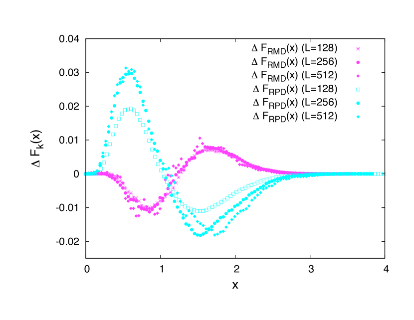
Figure 7: Differences $\Delta F_{k}(x)$ of cumulative distributions between disordered interfaces and Gaussian interfaces, for the depinning cases $k={\tt RMD,RPD}$, for system lengths $L=128,256,512$ for the disordered interfaces data, in average scaling.

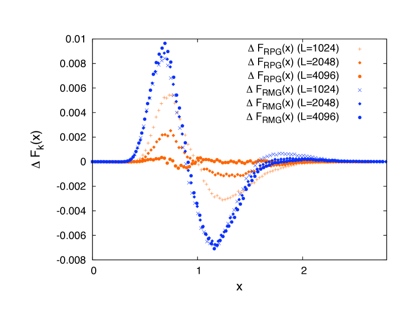
Figure 8: Differences $\Delta F_{k}(x)$ of cumulative distributions between disordered interfaces and Gaussian interfaces, for the ground-state cases $k={\tt RPG,RMG}$, for system lengths $L=1024,2048,4096$ for the disordered interface data, in average scaling.

To quantify the difference between the MRH distributions of elastic interfaces in random media and their corresponding Gaussian signal we start with a very simple statistical test. We assume that disordered elastic interfaces can be mapped onto a Gaussian signal by a simple rescaling of its amplitude by a factor $\chi$,

$$h(x)=\chi{\tilde{h}(x)},$$ (36)

and thus the two ensembles would be equivalent. This is indeed motivated by the analytical predictions for critical interfaces at depinning showing that the displacement field can be written as $u=\sqrt{\epsilon}u_{0}+\epsilon u_{1}$ where $u_{0}$ is a Gaussian random variable of order ${\cal O}(1)$ while $u_{1}$ is a random variable with non-Gaussian fluctuations, also of order ${\cal O}(1)$ width_frg . Since $h(x)$ and ${\tilde{h}(x)}$ describe a self-affine interface with the same roughness exponent $\zeta$ we must have, in particular,

$$\overline{h_{m}} = aL^{\zeta},\;\langle{\tilde{h}_{m}}\rangle={\tilde{a}}L^{\zeta}$$ (37)

$$\sqrt{\overline{(h_{m}-\overline{h_{m}})^{2}}} = bL^{\zeta},\;\sqrt{\langle(\tilde{h}_{m}-\langle\tilde{h}_{m}\rangle)^{2}\rangle}={\tilde{b}}L^{\zeta}.$$ (38)

For the particular case RPG the parameters of the Gaussian signal ${\tilde{a}}$ and ${\tilde{b}}$ corresponding to (1) can be obtained analytically, since in this case the MRH distribution is Airy distributed, since $\zeta_{\tt RPG}=1/2$. We get ${\tilde{a}}_{\tt RPG}=\sqrt{\pi/8}$, ${\tilde{b}}_{\tt RPG}=\sqrt{5/12-\pi/8}$. For the other cases, the Gaussian parameters can be obtained numerically for a finite number of modes. In order to avoid mixing size effects present in both, the disordered interfaces and Gaussian signals through the number of modes, we have evaluated ${\tilde{a}}$ and ${\tilde{b}}$ for a very large number of modes. We find indeed that the value ${\tilde{a}}/{\tilde{b}}$ converges faster to its assymptotic value for larger roughness exponents. We have thus fixed $L=4096$ modes for the Gaussian signals, assuring that the values ${\tilde{a}}$ and ${\tilde{b}}$ are almost numerically converged for the $\zeta=2/3$ case (and thus for all higher exponents). By making the hypothesis (36) we get

$$\overline{h_{m}} = \chi\langle{\tilde{h}_{m}}\rangle\Rightarrow\chi=\frac{a}{{\tilde{a}}}$$ (39)

$$\overline{(h_{m}-\overline{h_{m}})^{2}} = \chi^{2}\langle(\tilde{h}_{m}-\langle\tilde{h}_{m}\rangle)^{2}\rangle\Rightarrow\chi=\frac{b}{{\tilde{b}}}\;,$$ (40)

implying that $b/{\tilde{b}}=a/{\tilde{a}}$ if the hypothesis is true. To quantify the possible differences we can thus define the ratio

$$\Delta=\frac{(a/{\tilde{a}})-(b/{\tilde{b}})}{\min\left(a/{\tilde{a}},b/{\tilde{b}}\right)}\;,$$ (41)

for each case $k$. In Fig. 9 we show the evolution of $\Delta_{k}$ with the system size $L$ for all the cases, RMG, RPG, RMD, and RPD. As discussed above finite size effects come from $a$ and $b$ and not from ${\tilde{a}}$ and ${\tilde{b}}$. We can see that $\Delta_{k}<0$ for the random-periodic cases ($k={\tt RPG,RPD}$) and the ground-state of the random-manifold ($k=\texttt{RMG}$), while $\Delta_{k}>0$ for the random-manifold at depinning ($k={\tt RMD}$). It indicates that the variance of the average-rescaled MRH distribution for the disordered interface data $k=\texttt{RPG},\texttt{RMG},\texttt{RPD}$ is larger than the variance of the corresponding average-rescaled MRH distribution for the Gaussian data, and the opposite is true for the RMD case. Focusing on the size-dependence, we see that $\Delta_{\tt RMD}$ quickly saturate to values of order of $0.03-0.04$, while both $|\Delta_{\tt RMG}|$ and $|\Delta_{\tt RPD}|$ slightly increase and should converge as well to a non-zero value for large systems $L\to\infty$. On the other hand $|\Delta_{\tt RPG}|$ slowly decreases with $L$ and show no tendency to saturation towards a finite value. Interestingly, as we show in the inset of Fig. 9 we have that for the RPG case $|\Delta_{\tt RPG}|\approx L^{-\theta_{\tt RPG}}$, with $\theta_{\tt RPG}\approx 0.5$. We find that this power law behaviour is not proper to the disordered interface however: the corresponding Gaussian signal also follows a very close power law as a function of the number of modes, as its MRH distribution approaches the assymptotic Airy distribution.

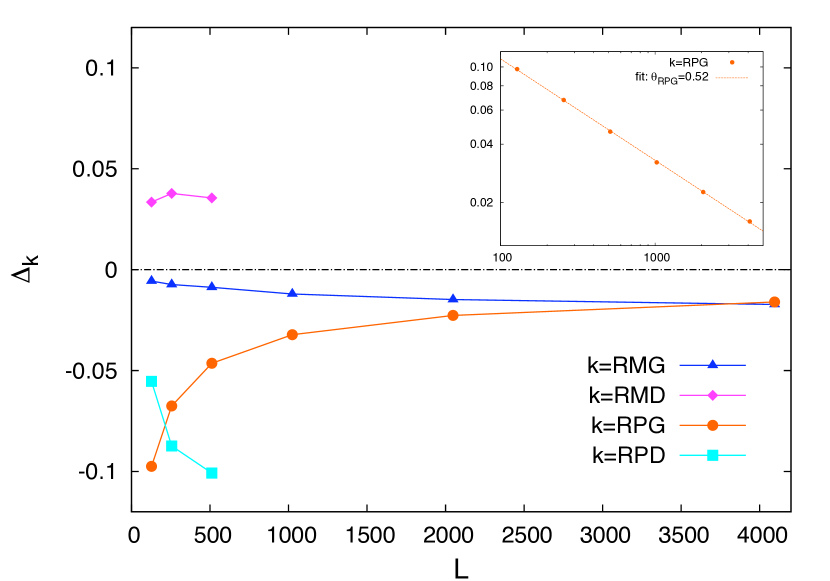
Figure 9: Values of ratios $\Delta_{k}$ for each case $k={\tt RMG,RMD,RPG,RPD}$ plotted with increasing size $L$ for the disordered interface data. The inset presents the power law behavior of $|\Delta_{\texttt{RPG}}|$ towards zero, in log-log scale.

To better quantify the non-Gaussian corrections we have performed a two sample Kolmogorov-Smirnov statistical test of equivalence between the MRH of sampled ground-states and their Gaussian approximations for the RMG and RPG cases. We have used the data sampled at the largest system sizes $L=2048,4096$ for both the disordered interfaces and Gaussian signals in order to reduce at maximum the possible finite-size effects in both processes. For the RMG we find a statistically significant difference between the distributions, with a probability less than $p<10^{-8}$ that the distributions are the same (null hypothesis). For RPG however, we find a probability or significance of order $p=0.5$ for $L=2048$, and $p=0.8$ for $L=4096$. It is thus very probable that the two distributions are the same one. Since the Gaussian case tends to the Airy distribution as $L\to\infty$ we conclude that the MRH statistics in the Random-Periodic class is in the same class as the one of periodic normal random-walks with $\zeta=1/2$. In this respect we note that this extends the study made in schehr_airy made for a family of thermally equilibrated Solid-on-Solid models without disorder, to a disordered system at $T=0$.

IV.4 Boundary conditions

The dependence on boundary conditions is a relevant issue. On the one hand it is experimentally usually difficult to realize prescribed boundary conditions for self-affine interfaces. In this respect a theory describing “window boundary conditions” have been recently proposed in which the width statistics of segments become universal and independent of boundary conditions raoul_width . On the other hand, boundary conditions usually add technical difficulties to the analytical approaches. Numerical studies with different boundary conditions are thus interesting, as they allow us to know the sensitivity to boundary conditions of different observables. Here we will address their effects on the MRH statistics for particular cases.

So far we have only analyzed self-affine periodic signals $h(0)=h(L)$ with a given period $L$, either originated from independent Fourier modes or from the interplay between local elasticity, disorder and a driving force, which all have stationary spatial correlation functions. This means for instance that for any two observables ${\cal O}_{1}(x)$ and ${\cal O}_{2}(x)$ the Gaussian signals considered satisfy $\langle{\cal O}_{1}(x){\cal O}_{2}(x^{\prime})\rangle\equiv\langle{\cal O}_{1}(0){\cal O}_{2}(x^{\prime}-x)\rangle$, while the considered critical configurations at depinning and ground-state configurations satisfy $\overline{{\cal O}_{1}(x){\cal O}_{2}(x^{\prime})}\equiv\overline{{\cal O}_{1}(0){\cal O}_{2}(x^{\prime}-x)}$. In particular, this implies that the MRH can occur, with uniform probability, at any position $x$.

Non-stationary spatial correlation functions can be easily generated using independent Fourier modes, while keeping the self-affine geometry, by applying different boundary conditions. For a self-affine signal $h(x)$ with roughness exponent $\zeta$ we can for instance impose fixed-ends $h(0)=h(L)=0$ by constructing a pure sine series ${\tilde{h}}(x)=\sum_{n=1}c_{n}\sin(n\pi x/L)$ with normally distributed uncorrelated amplitudes $c_{n}=N[0,(2/\pi n)(L/\pi n)^{\zeta}]$ wernerbook . It is easy to see that these signals have in general non-stationary spatial correlation functions. Consider, for instance, the observables ${\cal O}_{1}(x)={\cal O}_{2}(x)=h(x)-h(0)$: the correlation function $\langle{\cal O}_{1}(x){\cal O}_{2}(x^{\prime})\rangle$ vanishes for $x=0$ (or $x^{\prime}=0$) and $x=L$ (or $x^{\prime}=L$). In particular, it is clear that for fixed-ends the location of the MRH of each signal is not uniformly distributed along $L$: instead its pdf is peaked around $x=L/2$. The MRH distribution of these kind of non-stationary signals is not known exactly in general.

Ground-state configurations of elastic interfaces in random media can also have non-stationary spatial correlations functions in presence of certain constraints. Indeed we have seen that an optimal ground-state path with $h(0)=h(L)$ [note that we do not consider in this paper “tilted” signals with $h(0)\neq h(L)$] can be generated in two ways. The one we have analyzed so far comes from a minimization over all possible paths in the disordered substrate with $h(0)=h(L)$, and periodic boundary conditions in the displacements direction. This yields stationary ground-state configurations. On the other hand, if we do not seek the minimum among all possible paths such that $h(0)=h(L)$, but fix the extremity $h(0)=h(L)$ to a particular value we obtain ground-state configurations with non-stationary spatial correlation functions. In the two cases however, the self-affine structure is preserved, as it only depends on the variance of Fourier modes amplitudes rather than in its phases. Finally, let us note that the critical configurations at depinning we have analyzed have, by construction, stationary spatial correlation functions.

We will address here the effects of boundary conditions in the MRH distribution. To this purpose we focus on the well known directed polymer in a random medium, equivalent to the RMG case for our disordered elastic manifold. To illustrate the effects in this case we generate two particular types of boundary conditions by using the two methods outlined above to obtain both stationary and non-stationary ground-states with $\zeta=2/3$. One may write the height field as a fully periodic series, containing both cosines and sines as in Eq. (1) in the stationary case and as a sine series in the non-stationary case. We note that these boundaries conditions would give equivalent results for $\zeta=1/2$ wernerbook , which is the case of the RPG disordered interface.

In Fig. 10 we plot the difference of the cumulative MRH distributions in average scaling for the two cases, $\Delta F_{\texttt{RMG'}}(x)=F_{\texttt{RMG}}(x)-F_{\texttt{RMG'}}(x)$, where RMG and RMG’ denote the stationary and non-stationary ground-states respectively of the same size $L$, for $L=128,256,512$. We observe that for all sizes the difference is appreciable, of the same order than the difference between the RMG case and its Gaussian approximation, and it does not have any appreciable decrease with increasing $L$. We thus conclude that the MRH distribution of RM ground-states is sensitive to the boundary conditions.

In order to understand the origin of the sensitivity to boundary conditions we have also compared the MRH statistics of Gaussian interfaces described by the sine series (defined above) and by the full periodic series of Eq. (1). A Kolmogorov-Smirnov statistical test over $10^{6}$ averaged-scaled numerical Gaussian realizations shows that the MRH distribution for the sine series has, for $\zeta=1/2$, a probability $p\sim 0.9$ of being the same than the MRH distribution of the full-periodic series, while for $\zeta=2/3$ the same probability is $p\sim 10^{-11}$. While for $\zeta=1/2$ these results can be simply related to the fact that the signals are Markovian (and thus quickly loose “memory” of the border), for $\zeta=2/3$ they show that the dependence on boundary conditions is indeed closely related to the anomalous geometry, rather than to its particular microscopic origin or to the presence of non-Gaussian corrections. This extends the results obtained for the width distribution of Gaussian signals raoul_width to the case of the MRH.

Figure 10: Differences $\Delta F_{\texttt{RMG'}}(x)=F_{\texttt{RMG}}(x)-F_{\texttt{RMG'}}(x)$ of cumulative distributions between the two ways of selecting the optimal path in a disordered medium, for lengths $L=128,256,512$. The cumulative distributions are computed with average scaling, i.e. with $x=h_{m}/\overline{h_{m}}$.

V Conclusions

We have studied the maximal relative height statistics of self-affine one-dimensional elastic interfaces in a random potential. We have analyzed, by exact numerical sampling methods, the ground state configuration and the critical configuration at depinning, both for the experimentally relevant random-manifold and random-periodic universality classes. We have also analyzed the MRH distribution of self-affine signals generated by independent Gaussian Fourier modes and obtained an exact analytical description for the right tails using Pickands’ theorem. We found that in general, the independent Gaussian modes model provides a good approximation for predicting the MRH statistics, as it was previously found for the width distribution at depinning. This result is a priori not obvious as the MRH is an extreme observable (occurring at a single point in space for each realization) while the width is a spatially averaged one.

The comparison of the different MRH distributions with their approximation using Gaussian independent Fourier modes shows small differences that quickly saturate with system size in the case of depinning, in agreement with the results obtained for the width distribution of these configurations width_rosso ; width_frg : this confirms the predictions of non-Gaussian corrections at depinning. It would be very interesting to characterize more quantitatively these non-Gaussian corrections that we have observed for the MRH at the depinning threshold using the tools of Functional Renormalization Group review_frg . A preliminary analysis of this question indicates that this is not a simple extension of the previous works on the distribution of the width width_rosso ; width_frg : indeed the extension of the perturbation theory proposed in Refs. width_rosso ; width_frg to the computation of the MRH distribution involves, at lowest order, a constrained propagator (with an absorbing boundary at $h=0$) for which the Wick’s theorem does not hold.

On the other hand, for ground-state configurations we also find small differences but they display a slower decrease with system size. For the random-manifold ground-states a finite difference is found in the large size limit, implying non-Gaussian corrections. This is qualitatively consistent with analytical results obtained for other physical observables for the directed polymer in a random medium. For instance, the energy of the optimal polymer which is described by one of the Tracy-Widom distributions (associated to the Gaussian Unitary Ensemble or to the Gaussian Orthogonal Ensemble of random matrices depending on the geometry of the problem), which thus shows strong deviations from Gaussian fluctuations dprm . The random-periodic ground states on the other hand have a MRH distribution that is indistinguishable from the Airy distribution for the largest system sizes, as follows from studying its moments and by a Kolmogorov-Smirnov statistical test. This further confirms the universality of the Airy distribution for periodic signals with $\zeta=1/2$, as shown for a family of non-disordered thermally equilibrated one-dimensional solid-on-solid models schehr_airy . Our results are also consistent with previous results obtained for the related Solid-on-Solid model on a disordered substrate in $1+1$ dimensions (which belongs to the same universality class as RPG) solidonsolid . For this model with one free end, the ground state configuration can be constructed iteratively so that the height field behaves, on large scale, as a random walk with $\zeta=1/2$. Notice however that at variance with Ref. solidonsolid we have considered here periodic boundary conditions.

Finally, we have shown that MRH distributions are in general sensitive to boundary conditions. This might be important for experiments, where particular boundary conditions are difficult to realize or are not precisely known. In this respect it would be interesting to perform an analysis of the MRH statistics using the “window boundary conditions” or “segment statistics” proposed and applied to the width statistics in Ref. raoul_width .

Our results show that the MRH statistics provide a valuable tool to study experimental images of self-affine interfaces, such as magnetic domain walls or contact lines in partial wetting. In particular, it allows to infer information about the mechanisms behind the universal self-affine geometry, such as the disorder-induced coupling between Fourier modes, or more generally the one induced by non-linear interaction terms. It also allows to infer information about boundary conditions. Our results might be used as a guide for analytical approaches predicting the statistics of extreme geometrical observables.

Appendix A Pickands’ theorem and the right tail of the distribution of the MRH for a Gaussian path

Let $X(t)$, $t\in[0,T]$ be a continuous centered Gaussian process with covariance function $r(t)=\langle X(s)X(s+t)\rangle$ which satisfies

1. $r(t)\leq 1$, for $t\in[0,T]$  ,

2. $r(t)=1-C|t|^{\mu}+o(|t|^{\mu})$ as $t\to 0$    ,

where $T>0$, $\mu\in(0,2]$ and $C>0$ are constants. Let us define

$$X_{\max}=\max_{0\leq t\leq T}X(t)\;.$$ (42)

Pickands’ results concerns the right tail of the distribution of $X_{\max}$, ${\rm Pr}(X_{\max}\leq\xi)$ pickands :

$$\lim_{\xi\to\infty}\frac{{\rm Pr}(X_{\max}\geq\xi)}{\xi^{2/\mu}\Phi(\xi)}=TC^{1/\mu}H_{\mu}\;,$$ (43)

where $\Phi(\xi)=\frac{1}{\sqrt{2\pi}}\int_{\xi}^{\infty}e^{-u^{2}/2}$ and $H_{\mu}>0$, the so-called Pickands’ constant, is given by

$$H_{\mu}=\lim_{T\to\infty}T^{-1}\int_{0}^{\infty}e^{s}{\rm Pr}\left(\max_{0\leq t\leq T}Y(t)>s\right)\,{\mathrm{d}}s\;,$$

$$Y(t)=\sqrt{2}B_{\mu/2}(t)-t^{\mu}$$ (44)

where $B_{\mu/2}(t)$ is the fractional Brownian motion with Hurst exponent $\mu/2$, i.e. the Gaussian process characterized by the two-point correlation function:

$$\langle B_{\mu/2}(t)B_{\mu/2}(s)\rangle=\frac{1}{2}\left(t^{\mu}+s^{\mu}-|t-s|^{\mu}\right)\;.$$ (45)

No explicit formula exist for $H_{\mu}$ except for $\mu=1$ and $\mu=2$, for which $H_{1}=1$ and $H_{2}=1/\sqrt{\pi}$. The result above (43) means that the pdf of $X_{\max}$ behaves, for large argument as

$$\frac{d}{d\xi}{{\rm Pr}(X_{\max}\leq\xi)}\sim TC^{1/\mu}\frac{H_{\mu}}{\sqrt{2\pi}}\xi^{2/\mu}e^{-\frac{\xi^{2}}{2}}\;.$$ (46)

Here we will apply this result (46) to derive the asymptotic behavior of $h_{m}=\max_{0\leq x\leq L}h(x)$ where $h(x)$ is given in Eq. (1) and distributed according a Gaussian probability measure as in Eq. (12). We thus first compute the two-point correlation function as

$$\langle h(x)h(x^{\prime})\rangle=\frac{2L^{\alpha-1}}{(2\pi)^{\alpha}}\sum_{n=1}^{\infty}\frac{1}{n^{\alpha}}\cos{\left(\frac{2\pi n}{L}(x-x^{\prime})\right)},$$ (47)

which is obviously stationary. One has in particular ${\rm w}^{2}_{L}=\langle h(x)h(x)\rangle=\frac{2L^{\alpha-1}}{(2\pi)^{\alpha}}{\bm{\zeta}}(\alpha)$, independently of $x$. If one defines

$$\tilde{h}(x)=\frac{h(x)}{{\rm w}_{L}}\;,$$ (48)

then the two-point correlator is also stationary $r(x)=\langle\tilde{h}(y)\tilde{h}(y+x)\rangle$ and periodic $r(0)=r(L)$. In addition one has from Eq. (47) that it satisfies $r(x)\leq 1$, $\forall x\in[0,L]$. To apply Pickands’ theorem we need to analyze the small $x$ behavior of $r(x)$. To this purpose, it is useful to write $r(x)$ as

$$r(x)=\frac{1}{2\zeta(\alpha)}\left[{\rm Li}\left(\alpha,e^{2i\pi x/L}\right)+{\rm Li}\left(\alpha,e^{-2i\pi x/L}\right)\right]\;,$$ (49)

where ${\rm Li}(\alpha,x)$ is the polylogarithm function abramowitz . In particular, for $\alpha=2n$ one has abramowitz

$$r(x) = (-1)^{n+1}\frac{(2\pi)^{2n}}{2(2n)!{\bm{\zeta}}(2n)}B_{2n}(x)$$ (50)

$$= \frac{B_{2n(x)}}{B_{2n}(0)}\;,$$

where $B_{2n}(x)$ is the Bernoulli polynomial of degree $2n$ and $B_{2n}(0)={\rm b}_{2n}$ is a Bernoulli number, which satisfies ${\rm b}_{2n}=2(-1)^{n-1}{\bm{\zeta}}(2n)(2n)!/(2\pi)^{2n}$. Hence one has for instance, for $\alpha=2$

$$r(x)=1-6x+6x^{2}\;,$$ (51)

so that, in that case, $\mu=1$ while for $\alpha=4$ one has

$$r(x)=1-30x^{2}+60x^{3}-30x^{4}\;,$$ (52)

so that $\mu=2$ in that case. The small argument behavior of $r(x)$ can be obtained for any $\alpha$ from a careful asymptotic analysis of Eq. (49) which yields

$$r(x)\sim\begin{cases}&1-2\pi\frac{|\Gamma(1-\alpha)\sin{\frac{\alpha\pi}{2}}|}{{\bm{\zeta}}(\alpha)}x^{\alpha-1}\;,\;1<\alpha<3\>,\\ &1+\frac{2\pi^{2}}{{\bm{\zeta}}(3)}x^{2}\log{x}\;,\;\alpha=3\;,\\ &1-2\pi^{2}\frac{{\bm{\zeta}}(\alpha-2)}{{\bm{\zeta}}(\alpha)}x^{2}\;,\;\alpha>3\;.\end{cases}$$ (53)

It is then straightforward to use Pickands’ theorem (46) to obtain the results given in the text in Eqs (19, 20, 22, 21). Note that in the general case where $1<\alpha<3$, one obtains the amplitude $D$ as

$$D = \frac{H_{\alpha-1}}{\sqrt{2\pi}}\left(\frac{2\pi}{\zeta(\alpha)}\left|\Gamma(1-\alpha)\sin{\left(\frac{\alpha\pi}{2}\right)}\right|\right)^{1/(\alpha-1)}$$ (54)

$$\times \left(\frac{(2\pi)^{\alpha}}{2\zeta(\alpha)}\right)^{\frac{\alpha+1}{2(\alpha-1)}}$$

where $H_{\alpha-1}$ is the Pickands’ constant given in Eq. (A).

References

- (1) J.-P. Bouchaud and, M. Mézard, J. Phys. A 30, 7997 (1997).
- (2) G. Biroli, J.-P. Bouchaud, and M. Potters, J. Stat. Mech. P07019 (2007).
- (3) S. Raychaudhuri, M. Cranston, C. Przybyla, and Y. Shapir, Phys. Rev. Lett. 87, 136101 (2001).
- (4) S. N. Majumdar and A. Comtet, Phys. Rev. Lett. 92, 225501 (2004).
- (5) S. N. Majumdar and A. Comtet, J. Stat. Phys. 119, 777 (2005).
- (6) G. Schehr and S. N. Majumdar, Phys. Rev. E 73, 056103 (2006).
- (7) G. Györgyi, N. R. Moloney, K. Ozogány, and Z. Rácz, Phys. Rev. E 75, 021123 (2007).
- (8) J. Rambeau and G. Schehr, J. Stat. Mech. P09004 (2009).
- (9) J. Rambeau and G. Schehr, Europhys. Lett. 91, 60006 (2010); Phys. Rev. E 83, 061146 (2011).
- (10) A. L. Barabási and H. E. Stanley, ”Fractal concepts in surface growth” (Cambridge University Press, 1995).
- (11) T. Antal, M. Droz, G. Györgyi, and Z. Rácz, Phys. Rev. Lett. 87, 240601 (2001); Phys. Rev. E 65, 046140 (2002).
- (12) A. Rosso, W. Krauth, P. Le Doussal, J. Vannimenus, and K. J. Wiese, Phys. Rev. E 68, 036128 (2003).
- (13) P. Le Doussal and K. J. Wiese, Phys. Rev. E 68, 046118 (2003).
- (14) P. Le Doussal, Ann. Phys. 325, 49 (2010); K. J. Wiese and P. Le Doussal, Markov Processes Relat. Fields 13, 777 (2007).
- (15) S. Moulinet, A. Rosso, W. Krauth, and E. Rolley, Phys. Rev. E 69, 035103(R) (2004).
- (16) R. Santachiara, A. Rosso, and W. Krauth, J. Stat. Mech. P02009 (2007).
- (17) S. N. Majumdar, Current Science 89, 2076 (2005).
- (18) S. Lemerle, J. Ferré, C. Chappert, V. Mathet, T. Giamarchi, and P. Le Doussal, Phys. Rev. Lett. 80, 849 (1998); M. Bauer, A. Mougin, J. P. Jamet, V. Repain, J. Ferré, S. L. Stamps, H. Bernas, and C. Chappert, Phys. Rev. Lett. 94, 207211 (2005); M. Yamanouchi, D. Chiba, F. Matsukura, T. Dietl, and H. Ohno, Phys. Rev. Lett. 96, 096601 (2006).
- (19) P. Le Doussal, K. J. Wiese, S. Moulinet, and E. Rolley, Europhys. Lett. 87, 56001 (2009).
- (20) M. Alava, P. K. V. V. Nukalaz, and S. Zapperi, Adv. Phys. 55, 349 (2006); L. Ponson, D. Bonamy, and E. Bouchaud, Phys. Rev. Lett. 96, 35506 (2006); D. Bonamy, S. Santucci, and L. Ponson, Phys. Rev. Lett. 101, 045501 (2008).
- (21) T. Nattermann and S. Brazovskii, Adv. Phys. 53, 177 (2004).
- (22) G. Blatter, M. V. Feigelman, V. B. Geshkenbein, A. I. Larkin, and V. M. Vinokur, Rev. Mod. Phys. 66, 1125 (1994).
- (23) T. Giamarchi, S. Bhattacharya, in High Magnetic Fields: Applications in Condensed Matter Physics and Spectroscopy, Ed. C. Berthier et al. (Springer-Verlag, Berlin, 2002) p. 314, cond-mat/0111052.
- (24) A. B. Kolton, A. Rosso, T. Giamarchi, and W. Krauth Phys. Rev. B 79, 184207 (2009); Phys. Rev. Lett. 97, 057001 (2006).
- (25) M. Kardar, Nucl. Phys. B 290, 582 (1987); D. A. Huse, C. L. Henley, and D. S. Fisher, Phys. Rev. Lett. 55, 2924 (1985); M. Kardar and Y.-C. Zhang, Phys. Rev. Lett. 58, 2087 (1987); T. Halpin-Healy and Y.-C. Zhang, Phys. Rep. 254, 215 (1995).
- (26) S. Bustingorry, A. B. Kolton, and T. Giamarchi, Phys. Rev. B 82, 094202 (2010).
- (27) H. Rieger and U. Blasum, Phys. Rev. B 55, R7394 (1997).
- (28) A. Rosso, A. K. Hartmann, and W. Krauth, Phys. Rev. E 67, 021602 (2003).
- (29) S. Bustingorry and A. B. Kolton, Papers in Physics 2, 020008 (2010).
- (30) P. Chauve, T. Giamarchi, and P. Le Doussal, Phys. Rev. B 62, 6241 (2000).
- (31) J. Pickands III, Trans. Amer. Math. Soc. 145, 75 (1969).
- (32) M. Abramowitz and I. A. Stegun in Handbook of Mathematical Functions (Dover, New York, 1973).
- (33) L. Takacs, J. Appl. Prob. 32, 375 (1995).
- (34) S. Janson and G. Louchard, Elec. Journ. Prob. 12, 1600 (2007).
- (35) H. J. Hilhorst, P. Calka, and G. Schehr, J. Stat. Mech. P10010, (2008).
- (36) A. Rosso and W. Krauth, Phys. Rev. Lett. 87, 187002 (2001); A. Rosso and W. Krauth, Phys. Rev. B 65, 012202 (2002).
- (37) W. Krauth, Statistical Mechanics: Algorithms and Computations (Oxford University Press, Oxford, 2006) (See www.phys.ens.fr/doc/SMAC).
- (38) M. Prähofer and H. Spohn, Phys. Rev. Lett. 84, 4882 (2000); J. Stat. Phys. 108, 1071 (2002); K. Johansson, Comm. Math. Phys. 209, 437 (2000); P. Calabrese, P. Le Doussal, and A. Rosso, Europhys. Lett. 90, 20002 (2010); V. Dotsenko, Europhys. Lett. 90, 20003 (2010); P. Calabrese and P. Le Doussal, Phys. Rev. Lett. 106, 250603 (2011); P. J. Forrester, S. N. Majumdar, and G. Schehr, Nucl. Phys. B 844, 500 (2011).