Nonlinear Schrödinger equations with multiple-well potential

Abstract. We consider the stationary solutions for a class of Schrödinger equations with a $N$-well potential and a nonlinear perturbation.  By means of semiclassical techniques we prove that the dominant term of the ground state solutions is described by a $N$-dimensional Hamiltonian system, where the coupling term among the coordinates is a tridiagonal Toeplitz matrix.  In particular we consider the case of $N=4$ wells, where we show the occurrence of spontaneous symmetry-breaking bifurcation effect.  In particular, in the limit of large focusing nonlinearity we prove that the ground state stationary solutions consist of $N$ wavefunctions localized on a single well.

PACS number(s): 05.45.-a, 02.30.Oz, 03.65.Sq, 03.75.Lm

Keywords: Nonlinear dynamics, Bifurcation, Semiclassical limit, Bose-Einstein condensates in lattices

1 Introduction

For a quantum system with ${\mathcal{N}}$ particles the Schrödinger equation is defined in a space with dimension $3{\mathcal{N}}+1$ and typically it is impossible to solve, neither analytically nor numerically even with today’s supercomputers.  However, assuming a mean field hypothesis, the $3{\mathcal{N}}+1$ dimensions linear system of Schrödinger equation is approximated by a $3+1$ dimensions nonlinear Schrödinger equation.  Although nonlinearity typically implies some new technical difficulties, the dimension is significantly reduced when compared with the original problem and this fact simplifies the study of dynamics of quantum systems, independently of the total number ${\mathcal{N}}$ of particles.

One of the most successful application of such an approach is the derivation of nonlinear Schrödinger equation for a Bose-Einstein condensate (BEC).  Since its realization in diluted bosonic atomic gases [1, 4, 9] the interest in studying the collective dynamics of macroscopic ensembles of atoms occupying the same quantum state is largely increased.  The condensate typically consists of a few thousands to millions of atoms which are confined by a trapping potential and at temperature much smaller than some critical value, and a BEC is well described by the macroscopic wave function $\psi=\psi(x,t)$ whose time evolution is governed by a self-consistent mean field nonlinear Schrödinger equation [20]

Fos such a reason, in these last years there has been an increasing interest in the study of nonlinear Schrödinger equation with an external potential.  In fact, many other interesting and current physical problems may be described by means of such a model, e.g. non-linear optics [12], semiconductors [19], and quantum chemistry [7, 13], just to mention the most relevant.  In particular, the mathematical research recently focused on the nonlinear Schrödinger equation (hereafter NLS) with double well potential.  One of the most interesting feature of such a model is the spontaneous symmetry breaking phenomenon [11, 16, 21], and recently a general rule in order to classify the kind of bifurcation has been obtained [5, 22] (see also [15]).  Much less is known for NLS with multiple well potential.  So far, few models with multiple wells have been considered, e.g. the model with three wells on a regular lattice [14] (where a lattice means a sequence of points displaced along a straight line), and the model with four wells on the vertex of a regular square [24].  The generic case with $N$ wells has not been yet studied.  In fact, multiple-well potential represent the effect of small lattice on, e.g., Bose-Einstein condensates; furthermore, they are also interesting in order to understand the transition to a lattice with infinitely many wells.

In NLS problems with multi-well potentials the effective nonlinearity parameter is usually given by the ratio between the strength of the nonlinear term and hopping matrix element between neighbour sites.  The spontaneous symmetry breaking effect, and the associated localization phenomena, occurs when such a ratio is equal to a (finite) critical value.  This fact has been seen, for instance, in the study of the localization effect in a gas of pyramidal molecules as the ammonia one [13] or in the study of the Mott insulator-superfluid quantum phase transition [3, 23].  On the other side we also have to treat the problem of the validity of the $N$-mode approximation (where $N$ is the number of wells), obtained by restricting our analysis to the $N$-dimensional space associated to the first $N$ eigenvectors of the linear problem; in our approach we solve this problem considering the semiclassical limit of small $\hbar$.  Since the hopping matrix element between neighbour sites is not fixed, but it is exponentially small when $\hbar$ goes to zero, then, in order to have a finite value for the effective nonlinearity parameter (if not then we simply have localization), we have to require that the strength of the nonlinear term should be exponentially small, too.  Hence, in our model we introduce the multi-scale limit below in order to observe the bifurcation phenomena.  We would point out that other multi-scale limits may be considered in order to obtain the validity of the $N$-mode approximation, e.g. one can consider the simultaneous limit of large distance between the wells and small nonlinear term as in [15, 16].  The assumption of small $\hbar$ has the great advantage that, from a technical point of view, all the powerfull semiclassical results devoloped by Helffer and Sjöstrand in the 80’ (see e.g. [10]) are easily available when we consider the interaction between noighbour wells.

In this paper we consider a NLS with $N$ wells displaced on a regular lattice (even if the present analysis can be easily extended to the case on wells displaced on a regular grid, as discussed in an explicit example in Remark 3).  We’ll show that such a problem can be reduced, up to a remainder term, to a finite dimensional system; to this end, instead of using some kind of Galerkin decomposition as in [14], we assume to be in the semiclassical limit.  In such a way we can make use of some powerfull results of the semiclassical analysis [10].  By means of such results and by making us of the Lyapunov-Schmidt reduction scheme we estimate the remainder term.

The finite-dimensional system we obtain is almost decoupled, in the sense that the coupling term which represents the interaction among the adjacent wells is associated to a tridiagonal Toeplitz matrix.  Furthermore, it can be written in Hamiltonian form, where one of the coordinate is a cyclic coordinate.

We then consider in details the case of $N=4$ wells and we study the bifurcation picture when the strength of the nonlinear perturbation increases.  As in the double well model we can see that the ground state stationary symmetric solution bifurcates giving arise to $4$ stationary solutions fully localized on a single well, and the kind of bifurcation satisfies the same rule as in the double well model.  Actually, such a result may be generalized to any number $N$ of wells by means of a simple asymptotics argument.  In particular, we focus our attention on the value of the effective nonlinearity parameter at the bifurcation point in the case of $N=2,4,6$ and $8$ wells; indeed bifurcation phenomena is associated to the phase transition and we’ll see that the results obtained by our model agree with the numerical experiment on the Bose-Hubbard model [23].

Acknowledgments: I am very grateful to Reika Fukuizumi for useful discussions.

2 Description of the model

Here, we consider the nonlinear Schrödinger (hereafter NLS) equations

$$i\hbar\frac{\partial\psi}{\partial t}=H_{0}\psi+\epsilon g(x)|\psi|^{2\sigma}\psi,\ \psi(\cdot,t)\in L^{2}(\mathbbm{R}^{d},dx),\ \|\psi(\cdot,t)\|=1,$$ (1)

where $\epsilon\in\mathbbm{R}$ and $\|\cdot\|$ denotes the $L^{2}(\mathbbm{R}^{d},dx)$ norm,

$$H_{0}=-\frac{\hbar^{2}}{2m}\Delta+V,\ \ \ \Delta=\sum_{j=1}^{d}\frac{\partial^{2}}{\partial x_{j}^{2}}\,,$$ (2)

is the linear Hamiltonian with a multiple-well potential $V(x)$, and $g(x)|\psi|^{2\sigma}$ is a nonlinear perturbation.  For the sake of definiteness we assume the units such that $2m=1$.  The semiclassical parameter $\hbar$ is such that $\hbar\ll 1$.

Here, we introduce the assumptions on the multiple-well potential $V$ and we collect some semiclassical results on the linear operator $H_{0}$.

Hypothesis 1

Let $v(x)\in C^{\infty}_{0}(\mathbbm{R}^{d})$ be a smooth compact support function with a non degenerate minimum value at $x=0$:

$$v(x)>v_{min}=v(0),\ \ \forall x\in\mathbbm{R}^{d},\ x\not=0.$$ (3)

We consider multiple-well potentials of the kind

$$V(x)=\sum_{j=1}^{N}v(x-x_{j})$$ (4)

for some $N>1$, where

$$x_{j}=\left(j\ell-\frac{N+1}{2}\ell,0,\ldots,0\right)\,$$

and $\ell>2r$, where $r>0$ is such that

$${\mathcal{C}}\subseteq[-r,+r]\times\mathbbm{R}^{d-1}$$

and where ${\mathcal{C}}$ is the compact support of $v(x)$.

Hence, the multi-well potential $V(x)$ has exactly $N$ non degenerate minima at $x=x_{j}$, $j=1,2,\ldots,N$.

Remark 1

It is a well known fact [5] that the Cauchy problem (1) is globally well-posedness for any $\epsilon\in\mathbbm{R}$ small enough provided that

$$\sigma<\left\{\begin{array}[]{ll}+\infty&\ \mbox{ if }d<2\\ \frac{1}{d-2}&\ \mbox{ if }d>2\end{array}\right.\,.$$

In such a case the conservation of the norm of $\psi(x,t)$ and of the energy

$${\mathcal{E}}(\psi)=\langle\psi,H_{0}\psi\rangle+\frac{\epsilon}{\sigma+1}\langle\psi^{\sigma+1},g\psi^{\sigma+1}\rangle$$

follows; furthermore we also have a priori estimate

$$\|\psi(\cdot,t)^{2\sigma}\|\leq C\hbar^{-m}$$ (6)

for some positive constants $C$ and $m$.

3 Analysis of the linear Schrödinger equation

Now, making use of semiclassical analysis [10] we look for the ground state of the linear Schrödinger equation

$$H_{0}\psi=\lambda\psi,\ \ \psi\in L^{2}(\mathbbm{R}^{d})\,.$$

Let $d_{A}(x,y)$ be the Agmon distance between two points $x$ and $y$, let

$$S_{0}=\inf_{i\not=j}d_{A}(x_{j},x_{i});$$

then, by construction of the potential $V(x)$, it turns out that

$$S_{0}=d_{A}(x_{j},x_{j+1}),\ j=1,2,\ldots,N-1\,,$$ (7)

and

$$S_{0}<d_{A}(x_{j},x_{i})\ \mbox{ if }\ |i-j|>1\,.$$ (8)

Now, let $H_{D}$ be the Dirichlet realization of

$$H_{D}=-\hbar^{2}\Delta+v$$ (9)

on the ball $B_{S}(0)$ with center at $x=0$ and radius $S>2S_{0}$.  Since the bottom of $v(x)$ is not degenerate, then the Dirichlet problem associated to the single-well trapping potential $v(x)$ has spectrum $\sigma(H_{D})$ with ground state

$$\lambda_{D}=v(0)+\sum_{j=1}^{d}\sqrt{\mu_{j}}\hbar+{\mathcal{O}}(\hbar^{2})\,,$$

where $2\mu_{j}$ are the positive eigenvalues of the Hessian matrix $v^{\prime\prime}(0)$, such that

$$\mbox{dist}\left[\lambda_{D},\sigma(H_{D})\setminus\{\lambda_{D}\}\right]>2C\hbar$$

for some $C>0$; the associated normalized eigenvector $\psi_{D}(x)$ is localized in a neighborhood of $x=0$ and it exponentially decreases as ${\mathcal{O}}\left(\hbar^{-m}e^{-d_{A}(x)/\hbar}\right)$ for some $m>0$ and where $d_{A}(x)$ is the Agmon distance between $x$ and the point $x=0$.

The spectrum $\sigma(H_{0})$ of $H_{0}$ contains exactly $N$ eigenvalues $\lambda_{j}$, $j=1,2,\ldots,N$, such that

$$\lambda_{j}-\lambda_{D}={\mathcal{O}}(e^{-\rho/\hbar})$$

for any $0<\rho<S_{0}$; this result is a conseguence of the fact that the multiple well potential $V(x)$ is given by a superposition of $N$ exactly equal wells displaced on a regular lattice.  Furthermore

$$\mbox{dist}\left[\{\lambda_{j}\}_{j=1}^{N},\sigma(H_{0})\setminus\{\lambda_{j}\}_{j=1}^{N}\right]>C\hbar.$$

Let $F$ be the eigenspace spanned by the eigenvectors $\psi_{j}$ associated to the eigenvalues $\lambda_{j}$.  Then, the restriction $H_{0}|_{F}$ of $H_{0}$ to the subspace $F$ can be represented in the basis of orthonormalized vectors $\phi_{j}$ such that

$$\phi_{j}(x)-\varphi_{j}(x)={\mathcal{O}}\left(e^{-\rho/\hbar}\right)\,,\ j=1,2,\ldots,N,\ \varphi_{j}(x)=\psi_{D}(x-x_{j}),$$ (10)

for any fixed $0<\rho<S_{0}$; the eigenvector $\phi_{j}$ is localized in a neighborhood of the minima points $x_{j}$.  More precisely, $H_{0}|_{F}$ in the basis $\phi_{j}(x)$, $j=1,2,\ldots,N$, is represented by the $N\times N$ matrix (see, e.g. Theorem 4.3.4 by [10])

$$\lambda_{D}\mbox{\sc 1}_{N}+(w_{i,j})_{i,j=1}^{N}+{\mathcal{O}}(\hbar^{\infty})e^{-S_{0}/\hbar}$$ (11)

where

$$w_{i,j}=0\,,\ \mbox{ if }\ |i-j|\not=1,$$ (12)

and where

$$w_{i,i+1}=-\beta$$

is independent of $i=1,\ldots,N$ and it is such that (see Theorem 4.4.6 by [10])

$$\frac{1}{C}\hbar^{1/2}\leq\beta e^{S_{0}/\hbar}\leq C\hbar^{1-d/2}\,.$$ (13)

Remark 2

Let $i=1,\ldots,N-1$ be fixed and let $\Omega$ be an open set with smooth boundary such that $x_{i}\in\Omega$ and $x_{j}\notin\Omega$ for $i\not=j$, let

$$E_{i}^{(a)}=\left\{x\ :\ d_{A}(x_{i},x)+d_{A}(x_{i+1,x})\leq S_{0}+a\right\}$$

for some $a>0$ sufficiently small.  Let $\Gamma_{i}=\partial\Omega\cap E_{i}^{(a)}$, then

$$\beta=-\hbar^{2}\int_{\Gamma_{i}}\left[\psi_{D}(x-x_{i})\frac{\partial\psi_{D}(x-x_{i+1})}{\partial n}-\psi_{D}(x-x_{i+1})\frac{\partial\psi_{D}(x-x_{i})}{\partial n}\right]dS_{\Gamma}\,.$$ (14)

The dominant term of $\beta$ is independent of $a$.

In particular, in dimension one, i.e. $d=1$, then it turns out that

$$\beta=2\hbar^{2}\psi_{D}\left(\frac{1}{2}\ell\right)\psi_{D}^{\prime}\left(\frac{1}{2}\ell\right)\,.$$

Collecting all these results then we can conclude that

Lemma 1

Let $F$ be the eigenspace spanned by the eigenvectors $\psi_{j}$ associated to the eigenvalues $\lambda_{j}$ of $H_{0}$.  Then, the restriction $H_{0}|_{F}$ of $H_{0}$ to the subspace $F$ can be represented in the basis of vectors $\phi_{j}$, localized on the $j-$th well and satisfying (10), by the $N\times N$ tridiagonal Toeplitz matrix

$$T+{\mathcal{O}}(\hbar^{\infty})e^{-S_{0}/\hbar}$$ (15)

where

$$T=-\beta{\mathcal{T}}+\lambda_{D}\mbox{\sc 1}_{N}$$ (16)

and

$${\mathcal{T}}=\left(\begin{array}[]{cccccccc}0&1&0&0&0&0&\cdots&0\\ 1&0&1&0&0&0&\cdots&0\\ 0&1&0&1&0&0&\cdots&0\\ 0&0&1&0&1&0&\cdots&0\\ \vdots&\vdots&\vdots&\ddots&\ddots&\ddots&\vdots&\vdots\\ 0&\cdots&0&0&1&0&1&0\\ 0&\cdots&0&0&0&1&0&1\\ 0&\cdots&0&0&0&0&1&0\end{array}\right)\,.$$ (25)

where $\beta$ is the positive real number given by (14), and satisfying (13) for some $C>0$.

From (15) it turns out that the eigenvalues $\lambda_{j}$ are given, up to a small correction ${\mathcal{O}}(\hbar^{\infty})e^{-S_{0}/\hbar}$, by the eigenvalues $\mu_{j}$ of the matrix $T$.  To this end we recall that the $N$ eigenvalues of the tridiagonal Toeplitz matrix $T$ are given by [18]

$$\mu_{j}=\lambda_{D}-2\beta\cos\left(\frac{j\pi}{N+1}\right)\,,\ j=1,2,\ldots,N,$$

with associated eigenvectors

$$(v_{j})_{k}=\sin\left(\frac{kj\pi}{N+1}\right).$$

In order to normalize the eigenvector we remark that

$${\sum_{k=1}^{N}\sin^{2}\left(\frac{kj\pi}{N+1}\right)}=\frac{N+1}{2}$$

From this fact and from Lemma 1 we then conclude that

Lemma 2

The first $N$ eigenvalues $\lambda_{j}$ of $H_{0}$ are given by

$$\lambda_{j}=\lambda_{D}-2\beta\cos\left(\frac{j\pi}{N+1}\right)+{\mathcal{O}}(\hbar^{\infty})e^{-S_{0}/\hbar}\,,\ j=1,2,\ldots,N,$$

and the associated normalized eigenvector are given by

$$\psi_{j}(x)=\sum_{k=1}^{N}\alpha_{j,k}\varphi_{k}(x)+{\mathcal{O}}(\hbar^{\infty})e^{-S_{0}/\hbar}\,,\ j=1,2,\ldots,N,$$ (26)

where

$$\alpha_{j,k}=\alpha_{k,j}=\sqrt{\frac{2}{N+1}}\sin\left(\frac{kj\pi}{N+1}\right)\ \ \mbox{ and }\ \ \varphi_{k}(x)=\psi_{D}(x-x_{k}).$$

In the Appendix we’ll consider in detail the case of $N=2,3,4$ wells.

Remark 3

We can immediately extend such an analysis to multiple-well potentials of the form $V(x)=\sum_{j}v(x-x_{j})$ where $x_{j}\in\mathbbm{R}^{d}$ are points on a regular grid.  We study, for argument sake’s, the model in $\mathbbm{R}^{2}$ considered by [24] where the potential $V(x)$ has $4$ wells with minima on the points

$$x_{1}=(1,1);\ x_{2}=(1,-1);\ x_{3}=(-1,1);\ x_{4}=(-1,-1)\,.$$

In such a case we have that (recalling that $w_{i,j}=w_{j,i}$)

$$w_{1,2}=w_{1,3}=w_{2,4}=w_{4,3}=-\beta\ \mbox{ and }\ w_{i,i}=0,\ w_{1,4}=w_{2,3}=0\,$$

and the matrix $T$ takes the form

$$T=\left(\begin{array}[]{cccc}\lambda_{D}&-\beta&-\beta&0\\ -\beta&\lambda_{D}&0&-\beta\\ -\beta&0&\lambda_{D}&-\beta\\ 0&-\beta&-\beta&\lambda_{D}\end{array}\right)$$

with eigenvalues (and associated normalized eigenvectors $(v_{j})_{k}$)

$$\mu_{1} = \lambda_{D}-2\beta\,,\ v_{1}=\left(\frac{1}{2},\frac{1}{2},\frac{1}{2},\frac{1}{2}\right)$$

$$\mu_{2} = \lambda_{D}\,,\ v_{2}=\left(-\frac{1}{\sqrt{2}},0,0,\frac{1}{\sqrt{2}}\right)$$

$$\mu_{3} = \lambda_{D}\,,\ v_{3}=\left(0,-\frac{1}{\sqrt{2}},\frac{1}{\sqrt{2}},0\right)$$

$$\mu_{1} = \lambda_{D}-2\beta\,,\ v_{1}=\left(\frac{1}{2},-\frac{1}{2},-\frac{1}{2},\frac{1}{2}\right)$$

in agreement with [24].

4 The $N$-mode approximation for the NLS equation

Let $\psi$ be the normalized solution of the NLS equation (1) written in the form

$$\psi(x,t)=\sum_{j=1}^{N}c_{j}(t)\psi_{j}(x)+\psi_{c}(x,t)\,.$$ (28)

By substituting (28) into (1) and, projecting on the eigenspaces spanned by the eigenvectors $\psi_{j}$ and on the orthogonal eigenspace, we obtain the following system of differential equations:

$$\left\{\begin{array}[]{lcl}i\hbar\dot{c}_{j}&=&\lambda_{j}c_{j}+\epsilon\langle\psi_{j}(\cdot),g(\cdot)|\psi(\cdot,t)|^{2\sigma}\psi(\cdot,t)\rangle\\ i\hbar\dot{\psi}_{c}&=&H_{0}\psi_{c}+\epsilon\Pi_{c}g(x)|\psi(x,t)|^{2\sigma}\psi(x,t)\end{array}\right.$$ (31)

where we set

$$\Pi=\sum_{j=1}^{N}\langle\psi_{j},\cdot\rangle\psi_{j}\ \ \mbox{ and }\ \ \Pi_{c}=\mbox{\sc 1}-\Pi\,.$$

By substituting (26) in (31) we obtain

$$i\hbar\dot{c}_{j} = \lambda_{j}c_{j}+\epsilon\sum_{k}\bar{\alpha}^{j,k}\langle\varphi_{k}(\cdot),g(\cdot)|\psi(\cdot,t)|^{2\sigma}\psi(\cdot,t)\rangle+r_{k}$$

$$= \lambda_{j}c_{j}+\epsilon\sum_{k}\bar{\alpha}^{j,k}|d_{k}|^{2\sigma}d_{k}\langle\varphi_{k}(\cdot),g(\cdot)|\varphi_{k}(\cdot)|^{2\sigma}\varphi_{k}(\cdot)\rangle+r_{k}$$

$$= (\lambda_{D}+\omega_{j})c_{j}+\epsilon\sum_{k}\alpha^{j,k}C_{k}|d_{k}|^{2\sigma}d_{k}+r_{k}$$

where we set

$$d_{k}:=d_{k}(t)=\sum_{j=1}^{N}c_{j}(t)\alpha_{j,k}\,,$$ (32)

$$r_{k}=\epsilon\langle\varphi_{k}(\cdot),g(\cdot)|\psi_{c}(\cdot,t)|^{2\sigma}\psi_{c}(\cdot,t)\rangle+\epsilon{\mathcal{O}}(\hbar^{\infty})e^{-S_{0}/\hbar}\,,$$

$$\omega_{j}=-2\beta\cos\left(\frac{j\pi}{N+1}\right)\ \mbox{ and }\ C_{k}=\langle\varphi_{k}^{\sigma+1}(\cdot),g(\cdot)\varphi_{k}^{\sigma+1}(\cdot)\rangle\,,$$

since $\langle\varphi_{k},|\varphi_{m}|^{2\sigma}\varphi_{m}\rangle={\mathcal{O}}(\hbar^{\infty})e^{-S_{0}/\hbar}$ for $m\not=k$ and $\alpha_{j,k}=\bar{\alpha}_{j,k}=\alpha_{k,j}$, and where we make use of the a priori estimate (6) of the norm of $|\psi|^{2\sigma}$.  We should underline that, by construction and by Lemma 2, it follows that

$$\psi(x,t)=\sum_{k=1}^{N}d_{k}(t)\varphi_{k}(x)+\psi_{c}(x,t)+{\mathcal{O}}(\hbar^{\infty})e^{-S_{0}/\hbar}\,.$$

If we denote by

$$A=(\alpha_{j,k}),\ C=(C_{k}),\ d=(d_{k}),\ \lambda=\mbox{diag}(\lambda_{j}),\ r=(r_{k})_{k}\,,$$

then the above equation takes the form (with abuse of notation)

$$i\hbar A^{-1}\dot{d}=\Lambda A^{-1}d+\epsilon CA^{-1}|d|^{2\sigma}d+r$$

that is

$$i\hbar\dot{d}_{k}=(Td)_{k}+\epsilon\tilde{C}_{k}|d_{k}|^{2\sigma}d_{k}+\tilde{r}$$ (33)

since

$$T=A\Lambda A^{-1}$$

and where we set

$$\tilde{C}=ACA^{-1}\ \mbox{ and }\ \tilde{r}=Ar.$$

Definition 1

We call $N$-mode approximation for the NLS equation the system of ODEs obtained by neglecting the remainder term $\tilde{r}$

$$i\hbar\dot{d}_{k}=(Td)_{k}+\epsilon\tilde{C}_{k}|d_{k}|^{2\sigma}d_{k}\,,\ k=1,2,\ldots,N,$$ (34)

where $\tilde{C}_{k}$ are real-valued constant, and with the normalization condition

$$\sum_{k=1}^{N}|d_{k}(t)|^{2}=1\,.$$ (35)

The validity of the $N$-mode approximation for large times is, in general, an open problem .  So far it has been proved [2] that if the state is initially prepared on the space spanned by the $N$ linear eigenvectors then remainder term $\psi_{c}(\cdot,t)$ is norm bounded by an exponentially small term for times of order $\beta^{-1}$, furthermore the difference $c_{j}(t)-d_{j}(t)$, between the coefficients of the solution of the NLS equation and the solutions of the $N$-mode approximation, has the same exponentially small estimate for times of order $\beta^{-1}$ too.  This result can be extented for larger times of the order $e^{\beta^{-1}}$ under further technical assumptions.  Non linear systems (34) can be studied by means of dynamical systems methods, see [8] for the $N=2$ wells model.

Concerning the study of the stationary solutions $\psi(x,t)=e^{i\omega t}\psi(x)$ has been proved by [5] that the $2$-mode approximation gives the stationary solutions for the NLS, up to an exponentially small error, furthermore the orbital stability of the stationary solutions is proved; the same argument may apply to the $N$-mode approximation for any $N\geq 2$ proving that the stationary solutions of equations (34) and (35) give, up to an exponentially small error ${\mathcal{O}}(e^{-\rho/\hbar})$, for any $0<\rho<S_{0}$, the stationary solution of the NLS (1).  However, we don’t dwell here on these details.

For instance, in the case of two symmetric wells, i.e., $N=2$ then (34) takes the form (in agreement with [22])

$$\left\{\begin{array}[]{lcl}i\hbar\dot{d}_{1}&=&\lambda_{D}d_{1}-\beta d_{2}+\epsilon\tilde{C}_{1}|d_{1}|^{2}d_{1}\\ i\hbar\dot{d}_{2}&=&\lambda_{D}d_{2}-\beta d_{1}+\epsilon\tilde{C}_{2}|d_{2}|^{2}d_{2}\end{array}\right.$$

In the case of three symmetric wells, i.e., $N=3$ then (34) takes the form (in agreement with [14])

$$\left\{\begin{array}[]{lcl}i\hbar\dot{d}_{1}&=&\lambda_{D}d_{1}-\beta d_{2}+\epsilon\tilde{C}_{1}|d_{1}|^{2}d_{1}\\ i\hbar\dot{d}_{2}&=&\lambda_{D}d_{2}-\beta d_{1}-\beta d_{3}+\epsilon\tilde{C}_{2}|d_{2}|^{2}d_{2}\\ i\hbar\dot{d}_{3}&=&\lambda_{D}d_{3}-\beta d_{2}+\epsilon\tilde{C}_{3}|d_{3}|^{2}d_{3}\end{array}\right.$$

Finally, in the case of four symmetric wells, i.e., $N=4$ then (34) takes the form

$$\left\{\begin{array}[]{lcl}i\hbar\dot{d}_{1}&=&\lambda_{D}d_{1}-\beta d_{2}+\epsilon\tilde{C}_{1}|d_{1}|^{2}d_{1}\\ i\hbar\dot{d}_{2}&=&\lambda_{D}d_{2}-\beta d_{1}-\beta d_{3}+\epsilon\tilde{C}_{2}|d_{2}|^{2}d_{2}\\ i\hbar\dot{d}_{3}&=&\lambda_{D}d_{3}-\beta d_{2}-\beta d_{4}+\epsilon\tilde{C}_{3}|d_{3}|^{2}d_{3}\\ i\hbar\dot{d}_{4}&=&\lambda_{D}d_{4}-\beta d_{3}+\epsilon\tilde{C}_{4}|d_{4}|^{2}d_{4}\end{array}\right.$$ (42)

4.1 Hamiltonian form of the $N$-mode approximation

If we set

$$d_{k}=\sqrt{q_{k}}e^{i\theta_{k}},\ \ q_{k}\in[0,1]\,,\ \theta_{k}\in[0,2\pi)\,,$$

then, by means of a straightforward calculation, it follows that (34) takes the Hamiltonian form

$$\left\{\begin{array}[]{lcl}\hbar\dot{q}_{k}&=&\frac{\partial{\mathcal{H}}}{\partial\theta_{k}}=-2\beta\sum_{j=1}^{N}{\mathcal{T}}_{j,k}\sqrt{q_{k}q_{j}}\sin(\theta_{j}-\theta_{k})\\ \hbar\dot{\theta}_{k}&=&-\frac{\partial{\mathcal{H}}}{\partial q_{k}}=-\left[\lambda_{D}-\beta\sum_{j=1}^{N}{\mathcal{T}}_{j,k}\sqrt{\frac{q_{j}}{q_{k}}}\cos(\theta_{j}-\theta_{k})+\epsilon\tilde{C}_{k}q_{k}^{\sigma}\right]\end{array}\right.\,$$ (45)

with Hamiltonian function

$${\mathcal{H}} := {\mathcal{H}}(q_{1},\ldots,q_{N},\theta_{1},\ldots,\theta_{N})$$ (46)

$$= \lambda_{D}\sum_{k=1}^{N}q_{k}-\beta\sum_{j,k=1}^{N}{\mathcal{T}}_{k,j}\cos(\theta_{j}-\theta_{k})\sqrt{q_{j}q_{k}}+\epsilon\frac{1}{\sigma+1}\sum_{k=1}^{N}\tilde{C}_{k}q_{k}^{\sigma+1}$$

$$= \lambda_{D}\sum_{k=1}^{N}q_{k}-2\beta\sum_{k=1}^{N-1}\cos(\theta_{k+1}-\theta_{k})\sqrt{q_{k+1}q_{k}}+\epsilon\frac{1}{\sigma+1}\sum_{k=1}^{N}\tilde{C}_{k}q_{k}^{\sigma+1}\,.$$

The normalization condition (35) takes the form

$$\sum_{k=1}^{N}q_{k}=1\,,$$ (47)

furthermore the Hamiltonian function ${\mathcal{H}}$ is an integral of motion; i.e.

$${\mathcal{H}}\left[q_{1}(t),\ldots,q_{N}(t),\theta_{1}(t),\ldots,\theta_{N}(t)\right]=const.\,.$$ (48)

4.2 Reduced Hamiltonian

We make use of the fact that $\sum_{k}q_{k}=1$ in order to reduce from $N$ to $N-1$ the degree of freedom of the Hamiltonian system (46).  We consider the canonical transformation $(q,\theta)\to(Q,\Theta)$ defined as

$$Q_{h}=\sum_{k=1}^{h}q_{k}\,$$

where $Q_{1}\in[0,1]$ and $Q_{h}\in[0,1-Q_{h-1}]$, $h=2,\ldots,N-1$.  The inverse transformation is defined as

$$q_{1}=Q_{1}\ \mbox{ and }\ q_{h}=Q_{h}-Q_{h-1}\,,\ h=2,\ldots,N\,.$$

The associated transformation on the conjugate variable $\theta$ is then given by

$$\Theta_{N}=\theta_{N}\ \mbox{ and }\ \Theta_{h}=\theta_{h}-\theta_{h+1}\,,\ h=2,\ldots,N\,,$$

with inverse

$$\theta_{h}=\sum_{k=h}^{N}\Theta_{k}\,.$$

In the coordinates $(Q,\Theta)$ the Hamiltonian system takes the form

$$\left\{\begin{array}[]{lcl}\hbar\dot{Q}_{k}&=&\frac{\partial{\mathcal{K}}}{\partial\Theta_{k}}\\ \hbar\dot{\Theta}_{k}&=&-\frac{\partial{\mathcal{K}}}{\partial Q_{k}}\end{array}\right.\,,\ k=1,\ldots,N\,,$$ (51)

where the new Hamiltonian denoted by ${\mathcal{K}}$ is given by

$${\mathcal{K}} = {\lambda_{D}}Q_{N}-2\beta\cos(\Theta_{1})\sqrt{(Q_{2}-Q_{1})Q_{1}}-2\beta\sum_{k=2}^{N-1}\cos(\Theta_{k})\sqrt{(Q_{k+1}-Q_{k})(Q_{k}-Q_{k-1})}+$$

$$\ \ +{\epsilon}\frac{1}{\sigma+1}\left[\tilde{C}_{1}Q_{1}^{\sigma+1}+\sum_{k=2}^{N}\tilde{C}_{k}(Q_{k}-Q_{k-1})^{\sigma+1}\right]$$

It turns out hat $\Theta_{N}$ is a cyclic coordinate (indeed $Q_{N}=const.=1$), then the Hamiltonian system if finally given by

$$\left\{\begin{array}[]{lcl}\hbar\dot{Q}_{k}&=&\frac{\partial{\mathcal{K}}^{\star}}{\partial\Theta_{k}}\\ \hbar\dot{\Theta}_{k}&=&-\frac{\partial{\mathcal{K}}^{\star}}{\partial Q_{k}}\end{array}\right.\,,\ k=1,\ldots,N-1\,,$$ (54)

with Hamiltonian function

$${\mathcal{K}}^{\star} = {\lambda_{D}}-2\beta\cos(\Theta_{1})\sqrt{(Q_{2}-Q_{1})Q_{1}}-2\sum_{k=2}^{N-2}\cos(\Theta_{k})\sqrt{(Q_{k+1}-Q_{k})(Q_{k}-Q_{k-1})}-$$

$$\ \ -2\beta\cos(\Theta_{N-1})\sqrt{(1-Q_{N-1})(Q_{N-1}-Q_{N-2})}+$$

$$\ \ +{\epsilon}\frac{1}{\sigma+1}\left[\tilde{C}_{1}Q_{1}^{\sigma+1}+\sum_{k=2}^{N-1}\tilde{C}_{k}(Q_{k}-Q_{k-1})^{\sigma+1}+\tilde{C}_{N}(1-Q_{N-1})^{\sigma+1}\right]\,.$$

5 Stationary solutions

Now, we look for the normalized stationary solutions of the form $\psi(x,t)=e^{i\omega t}\psi(x)$.  In terms of $N$-mode approximation (46) it consists of looking for the solution of the system of equations

$$\left\{\begin{array}[]{lcl}0&=&\frac{\partial{\mathcal{H}}}{\partial\theta_{k}}\\ \hbar\omega&=&-\frac{\partial{\mathcal{H}}}{\partial q_{k}}\end{array}\right.\,,$$ (57)

That is, equation (57) and the normalization condition lead us to the following system

$$\left\{\begin{array}[]{lcl}-2\sin(\theta_{k+1}-\theta_{k})\sqrt{q_{k+1}q_{k}}+2\sin(\theta_{k}-\theta_{k-1})\sqrt{q_{k-1}q_{k}}&=&0\\ -2\sin(\theta_{N}-\theta_{N-1})\sqrt{q_{N}q_{N-1}}&=&0\\ +2\sin(\theta_{2}-\theta_{1})\sqrt{q_{2}q_{1}}&=&0\\ {\lambda_{D}}-\beta\left[\cos(\theta_{k+1}-\theta_{k})\sqrt{\frac{q_{k+1}}{q_{k}}}+\cos(\theta_{k}-\theta_{k-1})\sqrt{\frac{q_{k-1}}{q_{k}}}\right]+{\epsilon}\tilde{C}_{k}q_{k}^{\sigma}&=&-\hbar\omega\\ {\lambda_{D}}-\beta\cos(\theta_{N}-\theta_{N-1})\sqrt{\frac{q_{N-1}}{q_{N}}}+{\epsilon}\tilde{C}_{N}q_{N}^{\sigma}&=&-\hbar\omega\\ {\lambda_{D}}-\beta\cos(\theta_{2}-\theta_{1})\sqrt{\frac{q_{2}}{q_{1}}}+{\epsilon}\tilde{C}_{1}q_{1}^{\sigma}&=&-\hbar\omega\\ q_{1}+q_{2}+\ldots+q_{N}&=&1\end{array}\right.$$ (65)

where $k=2,\ldots,N-2$.

Remark 4

We may remark that from the first three equations of ( 65) it follows that

$$\sin(\theta_{k+1}-\theta_{k})\sqrt{q_{k+1}q_{k}}=0,\ \mbox{ for any }k=1,\ldots,N-1$$

Furthermore, from (34) the stationary solutions where $d_{1}\equiv 0$ and $d_{N}\equiv 0$ are not admitted, hence $|d_{k}|<1$ for any $k$.  Then $q_{1},q_{N}\in(0,1)$ and $q_{k}\in[0,1)$ for any $k=2,\ldots,N-1$.  For what concern the phases $\theta_{k}\in[0,2\pi)$ they are defined up to a gauge term, then we can always assume that, e.g., $\theta_{1}=0$.

5.1 Four wells

The stationary problem in the case of two wells and three wells have been already studied [5, 14, 22].  We restrict our analysis to the four-well case.  For the sake of definetness we consider the four-well ($N=4$) model where we assume that $g(x)$ is a constant function, hence $\tilde{C}_{k}$ is independent of $k$ and thus we set $C:=\tilde{C}_{k}=C_{k}$.  In such a case (65) takes the form

$$\left\{\begin{array}[]{lcl}\sin(\theta_{2}-\theta_{1})\sqrt{q_{2}q_{1}}&=&0\\ \sin(\theta_{3}-\theta_{2})\sqrt{q_{3}q_{2}}&=&0\\ \sin(\theta_{4}-\theta_{3})\sqrt{q_{4}q_{3}}&=&0\\ \frac{\lambda_{D}}{\beta}-\cos(\theta_{2}-\theta_{1})\sqrt{\frac{q_{2}}{q_{1}}}+\eta q_{1}^{\sigma}&=&-\omega\hbar/\beta\\ \frac{\lambda_{D}}{\beta}-\frac{1}{\sqrt{q_{2}}}\left[\cos(\theta_{3}-\theta_{2})\sqrt{q_{3}}+\cos(\theta_{2}-\theta_{1})\sqrt{q_{1}}\right]+\eta q_{2}^{\sigma}&=&-\omega\hbar/\beta\\ \frac{\lambda_{D}}{\beta}-\frac{1}{\sqrt{q_{3}}}\left[\cos(\theta_{4}-\theta_{3})\sqrt{q_{4}}+\cos(\theta_{3}-\theta_{2})\sqrt{q_{2}}\right]+\eta q_{3}^{\sigma}&=&-\omega\hbar/\beta\\ \frac{\lambda_{D}}{\beta}-\cos(\theta_{4}-\theta_{3})\sqrt{\frac{q_{3}}{q_{4}}}+\eta q_{4}^{\sigma}&=&-\omega\hbar/\beta\\ q_{1}+q_{2}+q_{3}+q_{4}&=&1\end{array}\right.$$ (74)

where we set

$$\eta=\frac{\epsilon}{\beta}C\,.$$

First of all we underline that $q_{2}=0$ (and similarly $q_{3}=0$) cannot be a solution of such a system; indeed if $d_{2}\equiv 0$ is a stationary solution of the $4$-mode approximation (42), then (42) reduces to

$$\left\{\begin{array}[]{lcl}i\hbar\dot{d}_{1}&=&\lambda_{d}d_{1}+\epsilon C|d_{1}|^{2}d_{1}\\ 0&=&-\beta d_{1}-\beta d_{3}\\ i\hbar\dot{d}_{3}&=&\lambda_{d}d_{3}-\beta d_{4}+\epsilon C|d_{3}|^{2}d_{3}\\ i\hbar\dot{d}_{4}&=&\lambda_{d}d_{4}-\beta d_{3}+\epsilon C|d_{4}|^{2}d_{4}\end{array}\right.$$

form which follows $d_{1}=d_{3}$ and then $d_{4}=0$, which is not possible since Remark 4.

Remark 5

We can extend such an argument to any $N$: if $N$ is an even integer and positive number then the stationary solution are given for $q_{k}\in(0,1)$, for any $k$.  If $N$ is an odd integer and positive number then the stationary solutions are given for $q_{1},q_{N}\in(0,1)$ and $q_{k}\in[0,1)$, $k=2,\ldots,N-1$, that is $q_{k}=0$, for $k\not=1,N$, may be admitted values for stationary solutions.

Since the stationary solutions are given for $q_{k}\in(0,1)$ then it follows that

$$\theta_{k+1}-\theta_{k}=0,\pi$$

and we obtain a family of $8$ systems of equations

$$\left\{\begin{array}[]{lcl}-(-1)^{j}\sqrt{\frac{q_{2}}{q_{1}}}+\eta q_{1}^{\sigma}&=&\Omega\\ -\frac{1}{\sqrt{q_{2}}}\left[(-1)^{\ell}\sqrt{q_{3}}+(-1)^{j}\sqrt{q_{1}}\right]+\eta q_{2}^{\sigma}&=&\Omega\\ -\frac{1}{\sqrt{q_{3}}}\left[(-1)^{m}\sqrt{q_{4}}+(-1)^{\ell}\sqrt{q_{2}}\right]+\eta q_{3}^{\sigma}&=&\Omega\\ -(-1)^{m}\sqrt{\frac{q_{3}}{q_{4}}}+\eta q_{4}^{\sigma}&=&\Omega\\ q_{1}+q_{2}+q_{3}+q_{4}&=&1\end{array}\right.\,,\ j,m,\ell=1,2.$$ (81)

where we set

$$\Omega=-\frac{\lambda_{D}+\hbar\omega}{\beta}\,.$$

5.2 Symmetric and antisymmetrical solutions

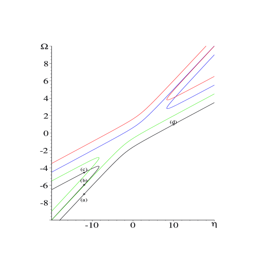
Figure 1: Here we plot the energy $\Omega$ corresponding to symmetrical/antisymmetrical solutions versus $\eta$ in the case of cubic nonlinearity (i.e. $\sigma=1$).  Black line corresponds to the choice $j=\ell=2$, and blue line corresponds to the choice $j=1$ and $\ell=2$, that is both graphs correspond to symmetric solutions; green line corresponds to the choice $j=2$ and $\ell=1$, ans, finally, red line corresponds to the choice $j=\ell=1$, that is both graphs correspond to antisymmetrical solutions.

In order to find symmetric and antisymmetrical solutions we set

$$q=q_{1}=q_{4}\ \mbox{ and }\ p=q_{2}=q_{3}$$

In such a case it follows that $m=j$, that is (81) reduces to

$$\left\{\begin{array}[]{lcl}-(-1)^{j}\sqrt{\frac{p}{q}}+\eta q^{\sigma}&=&\Omega\\ -\frac{1}{\sqrt{p}}\left[(-1)^{\ell}\sqrt{p}+(-1)^{j}\sqrt{q}\right]+\eta p^{\sigma}&=&\Omega\\ 2q+2p&=&1\end{array}\right.\,,\ j,\ell=1,2.$$ (85)

where to $j=2$ corresponds symmetric solutions, while to $j=1$ corresponds antisymmetrical solutions.

We see that the exchange $j\to 3-j$ reduces to the same system provided that $\eta\to-\eta$, $E\to-E$ and $\ell\to 3-\ell$; thus we can choose, for argument’s sake, $j=2$ obtaining

$$\left\{\begin{array}[]{lcl}-\sqrt{\frac{p}{q}}+\eta q^{\sigma}&=&E-\frac{1}{2}(-1)^{\ell}\\ -\sqrt{\frac{q}{p}}+\eta p^{\sigma}&=&E+\frac{1}{2}(-1)^{\ell}\\ 2q+2p&=&1\end{array}\right.\,,\ \ell=1,2.$$

where we set

$$\Omega=E-\frac{1}{2}(-1)^{\ell}\,.$$

It immediately follows that the exchange $\ell\to 3-\ell$ reduces to the same system provided we perform the exchange $p\leftrightarrow q$ and $E\to E+\frac{1}{2}(-1)^{\ell}$.  Therefore we can choose, for argument’s sake, $\ell=2$ and the system takes the final form

$$\left\{\begin{array}[]{lcl}-\sqrt{\frac{\frac{1}{2}-q}{q}}+\eta q^{\sigma}&=&E-\frac{1}{2}\\ -\sqrt{\frac{q}{{\frac{1}{2}-q}}}+\eta\left({\frac{1}{2}-q}\right)^{\sigma}&=&E+\frac{1}{2}\end{array}\right.\,.$$ (89)

By means of a straightforward calculation we can obtain $\eta$ and $\Omega$ as functions on $q$ and plot $\Omega$ versus $\eta$.

Figure 2: Here we plot the absolute value of the symmetric wavefunctions corresponding to the case $j=\ell=2$ for $\eta=-12$ and $\eta=10$, in the case of cubic nonlinearity.  For $\eta=-12<-\eta^{1}$ we have a wavefunction (a), which is the continuation of the unperturbed one, plus two new wavefunctions (b) and (c) associated to branches coming from a saddle point; for $\eta=10$ we only have the wavefunction (d), which is the continuation of the unperturbed one.

In Figure 1 we consider the value of $\Omega$, as function of $\eta$, corresponding to symmetric/antisymmetrical stationary solutions in the cubic case, where $\sigma=1$.  We may see that there exists a critical value $\eta^{1}=8.324$ such that for any $|\eta|<\eta^{1}$ we only have $4$ symmetric/antisymmetrical stationary solutions as in the linear case (where $\eta=0$).  At $\eta=\pm\eta^{1}$ saddle points occur and new branches of symmetric/antisymmetrical stationary solutions arise.  The points denoted by (a), (b), and (c) correspond to values of $\Omega$ for $\eta=-12<-\eta^{1}$ and where $j=\ell=2$; the point denoted by (d) corresponds to the unique value of $\Omega$ for $\eta=10$ and where $j=\ell=2$.  In particular we have that (see also Figure 2)

$$\begin{array}[]{llll}(a)&\eta=-12&\Omega=-7.021&q=0.010\\ (b)&\eta=-12&\Omega=-5.952&q=0.478\\ (c)&\eta=-12&\Omega=-4.534&q=0.314\\ (d)&\eta=10&\Omega=0.990&q=0.214\end{array}$$ (94)

We may remark that in the limit $|\eta|\to+\infty$, that is for large nonlinearity, then the wavefunctions (a) and (b) are, respectively, fully localized on the internal and external two wells, while the wavefunctions (c) and (d) are equally distributed on the four wells.

Remark 6

We should remark that the same picture occurs even for other values of $\sigma$; for instance in the case of $\sigma=2$ the saddle point occurs at $\eta=\eta^{2}=-16.648$, in the case of $\sigma=3$ the the saddle point occurs at $\eta=\eta^{3}=-38.775$.  In general, computing $\eta^{\sigma}$ for higher values of $\sigma$ the following rule appears: $\eta^{\sigma+1}/\eta^{\sigma}\sim 2$ for large $\sigma$.

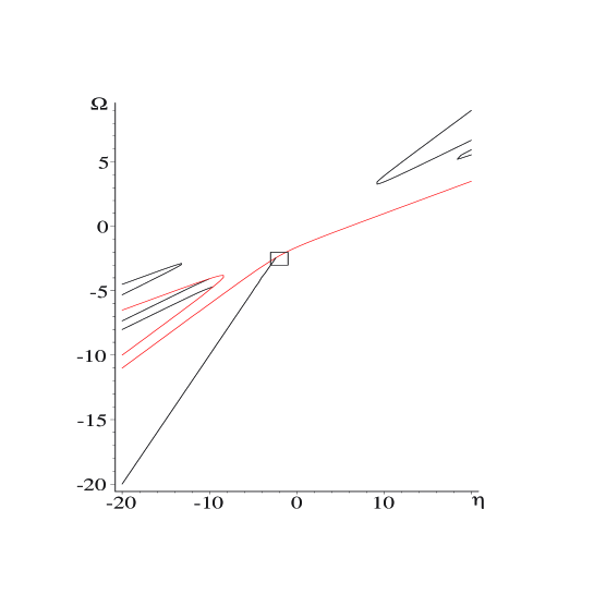
Figure 3: Here we plot the energy $\Omega$ corresponding to symmetric (red lines) and asymmetrical (black lines) solutions versus $\eta$ in the case of cubic nonlinearity (i.e. $\sigma=1$).  Here we choice $j=\ell=m=2$.  The symmetric ground state bifurcates at $\eta=-2.31$ and new asymmetrical solutions occur.  The bifurcation point, enclosed in the box, will be zoomed in Fig. 4.

5.3 Asymmetrical solutions

Now, we look for the asymmetrical solutions (81); actually, we have a family of $8$ different systems of equations.  In fact, we restrict our attention to the branches of asymmetrical solutions connected to the symmetric ground state.  To this end we choose $j=\ell=m=2$.  The numerical solutions of (81) in the cubic case (i.e. for $\sigma=1$) are plotted in Figure 3; more precisely we plot the energy $\Omega$ as function of $\eta$.  As appears in the piucture, branches of solution occurred when the effective nonlinearity parameter $\eta$ assumes critical values.  Among these branches we restrict our attention to the branch with bifurcates from the symmetric stationary solution (we zoom the bifurcation in details in Figure 4 for different values of the nonlinearity power $\sigma$).  As we can see a supercritical bifurcation of the symmetric stationary solution occurs at $\eta\approx-2.31$, the new branch behaves as $\Omega\approx\eta$ for large value of $|\eta|$, and the four almost-degenerate eigenfunctions are fully localized on one single well (as turns out in Table 1).

$\Omega$	$q_{1}$	$q_{2}$	$q_{3}$	$q_{4}$
-12.000  ($\mbox{e}_{1}$)	0.5$\cdot 10^{-5}$	0.007	0.986	0.007
-12.000  ($\mbox{e}_{2}$)	0.007	0.986	0.007	0.5$\cdot 10^{-5}$
-11.999  ($\mbox{e}_{3}$)	0.3$\cdot 10^{-6}$	0.5$\cdot 10^{-5}$	0.007	0.993
-11.999  ($\mbox{e}_{4}$)	0.993	0.007	0.5$\cdot 10^{-5}$	0.3$\cdot 10^{-6}$
-7.021  (a)	0.010	0.490	0.490	0.010
-7.009	0.2$\cdot 10^{-3}$	0.011	0.487	0.502
-7.009	0.502	0.487	0.011	0.2$\cdot 10^{-3}$
-5.979	0.013	0.451	0.069	0.466
-5.979	0.466	0.069	0.451	0.013
-5.952  (b)	0.478	0.022	0.022	0.478
-5.376	0.013	0.364	0.240	0.382
-5.376	0.382	0.240	0.364	0.013
-4.682	0.347	0.091	0244	0.317
-4.682	0.317	0.244	0.091	0.347
-4.534  (c)	0.314	0.186	0.186	0.314

Table 1: Here we collect all the solutions corresponding to the value $\eta=-12$.  Wavefunctions labeled with the letter (a), (b) and (c) coincides with the symmetrical ones already computed in (94); the other wavefunctions are asymmetrical wavefunctions.  In particular the $4$ wavefunctions ($\mbox{e}_{1}$)-($\mbox{e}_{1}$) associated to the ground state $\Omega\sim-12$ are fully localized on one single well

We may remark that (see also Figure 4, left panel) that the bifurcation is of the same supercritical kind as in the double well model (where bifurcation occurs at $\eta=-2$); furthermore, as in double well model, we observe (see also Figure 4, right panel) a subcritical bifurcation of the symmetric stationary solution when the value of the nonlinearity power is bigger than the critical value $\sigma_{threshold}=\frac{3+\sqrt{3}}{2}$ obtained by [22].  In adjoint to this spontaneous symmetry breaking effect of the ground state, which is the most relevant effect, other spontaneous symmetry breaking effect of the higher energy stationary states occur, and also new branches, associated to saddle points, of asymmetrical stationary states arise (see Figure 3 again).

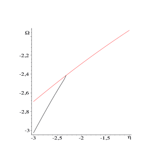
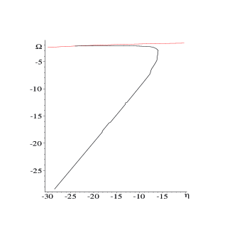
Figure 4: In the left picture we zoom the bifurcation point in the cubic case, i.e. $\sigma=1$.  For large value of $\sigma$ the kind of bifurcation may change; in the right picture we plot the bifurcation point for $\sigma=4$.  Red lines denote the symmetric stationary solutions, black lines denote the branch of the asymmetrical stationary solutions.

5.4 Ground state solution for large nonlinearity

As discussed above, we have seen that for $|\eta|$ large enough (actually $\eta=-12$, as computed in Table 1) the four almost-degenerate asymmetrical solutions, associated to the branch which bifurcates from the symmetric ground state, are localized on one single well.  This result can be proved by means of a simple asymptotic argument as $\eta\to-\infty$.  More precisely, let $j=m=\ell=2$ and let us set

$$q_{1}=1+\eta^{-2}s_{1}\ \mbox{ and }\ \Omega=\eta\left(1+\eta^{-2}\Gamma\right)$$

where $s_{1}=s_{1}(\eta)$ and $\Gamma=\Gamma(\eta)$ will be discussed later.  From equation (81-5) it follows that $q_{k}={\mathcal{O}}(\eta^{-2})$, $k=2,3,4$; more precisely, from equations (81-2), (81-3) and (81-4) immediately follows that

$$q_{2}=\eta^{-2}s_{2},\ q_{3}=\eta^{-4}s_{3}\ \mbox{ and }\ q_{4}=\eta^{-6}s_{4}$$

where $s_{k}:=s_{k}(\eta)$ are such that $s_{4}\sim s_{3}\sim s_{2}$, as $\eta\to-\infty$, and where $s_{2}\sim 1$, as $\eta\to-\infty$.  Since equations (81-1) and (81-5) imply that

$$s_{1}+s_{2}\sim 0\ \mbox{ and }\ \sqrt{s2}+\sigma s_{1}-\Gamma\sim 0\,,\ \mbox{ as }\ \eta\to-\infty\,,$$

hence

$$s_{1}\sim-1\ \mbox{ and }\ \Gamma\sim 1-\sigma\,.$$

This solution corresponds to the ground state, indeed it minimizes the Hamiltonian function (46) since $\sum_{k}q_{k}^{\sigma+1}\leq\left[\sum_{k}q_{k}\right]^{\sigma+1}$ and $|\epsilon/\beta|$ is large enough (because we are considering the case $|\eta|\gg 1$).

Since a similar argument may apply when we choose, as starting point, $q_{k}=1+\eta^{-2}s_{k}$, for $k=2,3,4$, then we have proved the following result.

Theorem 1

There exists a value $\eta^{\star}>0$ such that the symmetrical stationary ground state bifurcates at $\eta=-\eta^{\star}$ and in the limit of large focusing nonlinearity, that is $\eta\to-\infty$, then and the four almost-degenerate asymmetrical solutions, which arise at the bifurcation point, are localized on one single well.

Remark 7

We can extend this result to any number $N$ of wells; indeed the same asymptotic argument applies to the system (65) where we choose $\theta_{k}=\theta_{k+1}$ for any $k=1,2,\ldots,N-1$.

Remark 8

By making use of the same arguments in [5] one may prove that the resulting almost-degenerate asymmetrical stationary solutions are orbitally stable; however we don’t dwell here these details.

6 Conclusion

Semiclassical methods turn out to be a very powerfull tool in order to reduce a NLS to a finite-dimensional Hamiltonian systems.  Indeed, by applying such techniques jointly with the Lyapunov-Schmidt reduction scheme, we are able to describe the ground state solutions as a superposition of vectors localized on single wells, with a rigorous estimate of the error [5].  In particular the Hamiltonian system (45) we obtain it is explicitely written, it can be reduced and it can be studied by means of standard numerical tools.

In more details we consider the case with $N=4$ wells and we see that the spontaneous symmetry breaking effect, already observed in a double well model, similarly occurs; in particular we still observe supercritical bifurcation when the nonlinearity parameter is less that a threshold value, for value bigger that such a threshold value a subcritical bifurcation occurs.

A remarkable result is that in the case of large enough focusing nonlinearity then the symmetric ground state bifurcates and the new $N$ almost-degenerate stable solutions are fully localized on one single well.  This fact is very relevant from a physical point of view, indeed it is connected to, e.g. the explanation of the phase transition from superfluid to Mott-insulator state in the Bose-Hubbard model.  Indeed, we can see in Fig. 3 a smooth transition from superfluidity (which corresponds to stationary solutions distributed on the whole lattice) to Mott insulator phase (which corresponds to stationary solutions localized on a single lattice cell without possibility to jump from one site to the others); the phase transition appears to be concentrated around to the values of $\eta_{bif}$ corresponding to the bifurcation point.  in Table 2 we compute, for different values of the number $N$ of wells, the value of $\eta_{bif}$ for which we have a smooth transition from superfluidity to Mott insulator state, and we see that our results agree with the value of $\eta_{bif}\approx-1.8$ predicted by means of experimental calculation [23] .

$N$	2	4	6	8
$\eta_{bif}$	$-2.00$	$-2.29$	$-2.37$	$-2.33$

Table 2: Table of values for $\eta$ at which the symmetric stationary solution for the Gross-Piatevskii equation, with lattice potential with $N$ wells, bifurcates.

Appendix A Appendix

Here we compute the eigenfunctions (26) for the linear problem in the case of $N=2,3,4$ wells and where we assume, for argument’s sake, the dimension $d=1$ and where the multiple well potential is given by a superposition of exactly equal and symmetric $N$ wells (i.e. $v(x)=v(-x)$).  In sucha case the eigenvectors $\psi_{j}(x)$ are even and odd-parity functions.

In the case of two wells, i.e. $N=2$, then the two eigenvalues are given by

$$\lambda_{1}=\lambda_{D}-\beta\ \ \mbox{ and }\ \ \lambda_{2}=\lambda_{D}+\beta$$

and the matrix $A=(\alpha_{j,k})$ has the form (in agreement with [22])

$$A=\frac{\sqrt{2}}{2}\left(\begin{array}[]{cc}1&1\\ 1&-1\end{array}\right).$$

In the case of three wells, i.e. $N=3$, then

$$\lambda_{1}=\lambda_{D}-\sqrt{2}\beta\,,\ \lambda_{2}=\lambda_{D}\ \ \mbox{ and }\ \ \lambda_{3}=\lambda_{D}+\sqrt{2}\beta$$

and (in agreement with [14])

$$A=\frac{1}{2}\left(\begin{array}[]{ccc}1&\sqrt{2}&1\\ \sqrt{2}&0&-\sqrt{2}\\ 1&-\sqrt{2}&1\end{array}\right).$$

In the case of four wells, i.e. $N=4$, then

$$\lambda_{1} = \lambda_{D}-2\beta\cos\left(\frac{\pi}{5}\right)\,,\ \lambda_{2}=\lambda_{D}-2\beta\cos\left(\frac{2\pi}{5}\right)$$

$$\lambda_{3} = \lambda_{D}+2\beta\cos\left(\frac{2\pi}{5}\right)\,,\ \lambda_{4}=\lambda_{D}+2\beta\cos\left(\frac{\pi}{5}\right)$$

and

$$A=\frac{\sqrt{10}}{5}\left(\begin{array}[]{cccc}\sin(\pi/5)&\sin(2\pi/5)&\sin(2\pi/5)&\sin(\pi/5)\\ \sin(2\pi/5)&\sin(\pi/5)&-\sin(\pi/5)&-\sin(2\pi/5)\\ \sin(2\pi/5)&-\sin(\pi/5)&-\sin(\pi/5)&\sin(2\pi/5)\\ \sin(\pi/5)&-\sin(2\pi/5)&\sin(2\pi/5)&-\sin(\pi/5)\end{array}\right).$$

For instance, see Figures 1, 2 and 3 for the one-dimensional $N$-wells problem with, respectively, $N=2$, $N=3$ and $N=4$; where the wavefunctions $\psi_{D}(x)$ and $\psi_{j}(x)$ can be chosen to be real-valued functions.

Figure 5: Double-well potential (left) and the two symmetric and antisymmetrical eigenvectors (right).

Figure 6: Three-well potential (left) and the three symmetric and antisymmetrical eigenvectors (right).

Figure 7: Four-well potential (left) and the four symmetric and antisymmetrical eigenvectors (right).

References

- [1] Anderson, M.H., Ensher, J.R., Matthews, M.R., Wieman, C.E. and Cornell, E.A. Observation of Bose-Einstein Condensation in a Dilute Atomic Vapor. Science 269, 198-201 (1995).
- [2] D.Bambusi, and A.Sacchetti, Exponential times in the one-dimensional Gross-Pitaevskii equation with multiple well potential, Comm. Math. Phys. 275, 1-36 (2007).
- [3] Bloch I. Ultracold quantum gases in optical lattices. Nature Physics 1, 23-30 (2005).
- [4] Bradley, C.C., Sackett, C.A. and Hulet, R.G. Bose-Einstein condensation of lithium: Observation of limited condensate number. Phys. Rev. Lett. 78, 985-989 (1997).
- [5] R.Fukuizumi, and A.Sacchetti, Bifurcation and stability for Nonlinear Schrödinger equations with double well potential in the semiclassical limit, preprint (2011)
- [6] Z.Gang, and M.I.Weinstein, Equipartition of mass in nonlinear Schrd̈inger/Gross-Pitaevskii equations, Appl. Math. Res. Express 2011, 123-181 (2011).
- [7] V.Grecchi, and A.Martinez, Non-linear Stark effect and molecular localization, Comm. Math. Phys. 166, 533-548 (1995).
- [8] V.Grecchi, A.Martinez, and A.Sacchetti, Destruction of the beating effect for a non-linear Schrödinger equation, Comm. Math. Phys. 227, 191-209 (2002).
- [9] Hall, D.S., Mattthews, M.R., Ensher, J.R., Wieman, C.E. and Cornell, E.A. Dynamics of component separation in a binary mixture of Bose-Einstein condensates. Phys. Rev. Lett. 81, 1539-1542 (1998).
- [10] B.Helffer, Semi-classical Analysis for the Schrödinger operator and applications, Lecture Note in Mathematics, 1336, Springer-Verlag (1980).
- [11] R.K.Jackson, and M.I.Weinstein, Geometric Analysis of Bifurcation and Symmetry Breaking in a Gross-Pitaevskii Equation, J. Stat. Phys. 116, 881-905 (2004).
- [12] J.D.Joannopoulus, S.G.Johnson, J.N.Winn, and R.D.Meade, Photonic Crystals: molding the flow of light, (Princeton Univ. Press: 2008)
- [13] G.Jona-Lasinio, C.Presilla, and C.Toninelli, Interaction induced localization in a gas of pyramidal molecules, Phys.Rev.Lett. 88, 123001 (2002).
- [14] T.Kapitula, P.G.Kevrekidis, and Z.Chen, Three is a crowd: solitary waves in photorefractive media with three potential wells, SIAM J. Appl. Dyn. Syst. 5, 598-633 (2006).
- [15] E.W. Kirr, P.G. Kevrekidis, and D.E. Pelinovsky, Symmetry-breaking bifurcation in the nonlinear Schrodinger equation with symmetric potentials, Communications in Mathematical Physics (2011).
- [16] E.W.Kirr, P.G.Kevrekidis, E.Shlizerman, and M.I.Weinstein, Symmetry-breaking bifurcation in nonlinear Schrödinger/Gross-Pitaevskii equations, SIAM J. Math. Anal. 40, 566-604 (2008).
- [17] J.Marzuola, and M.I.Weinstein, Long time dynamics near the symmetry breaking bifurcation for nonlinear Schrödinger / Gross-Pitaevskii equations, Discrete and Continuous Dynamical Systems B 28, 1505-1547 (2010).
- [18] C.D.Meyer, Matrix analysis and applied linear algebra, SIAM (2004).
- [19] D.Mihalace, M.Bertolotti, and C.Sibilia, Nonlinear wave propagation in planar structures, Prog. Opt. 27, 229 (1989)).
- [20] L.Pitaevskii, and S.Stringari, Bose-Einstein condensation, (Claredon Press: Oxford 2003).
- [21] A.Sacchetti, Nonlinear double well Schrödinger equations in the semiclassical limit, J. Stat. Phys. 119, 1347-1382 (2005).
- [22] A.Sacchetti, Universal critical power for nonlinear Schrödinger equations with a symmetric double well potential, Phys. Rev. Lett. 103, 194101 (2009).
- [23] Stöferle, T., Moritz, H., Schori, C., Köhl, M. and Esslinger T. Transition from a Strongly Interacting 1D Superfluid to a Mott Insulator. Phys. Rev. Lett. 92 (2004), 130403:1-4.
- [24] C.Wang, G.Theocharis, P.G.Kevrekidis, N.Whitaker, K.J.H.Law, D.J.Frantzeskakis, and B.A.Malomed, Two-dimensional paradigm for symmetry breaking: the nonlinear Schrödinger equation with a four-well potential, Phys. Rev. E 80, 046611 (2009).