Hierarchical Bayesian estimation of inequality measures with nonrectangular censored survey data with an application to wealth distribution of French households

Abstract

We consider the estimation of wealth inequality measures with their confidence interval, based on survey data with interval censoring. We rely on a Bayesian hierarchical model. It consists of a model where, due to survey sampling and unit nonresponse, the summaries of the wealth distribution of households are observed with error; a mixture of multivariate models for the wealth components where groups correspond to portfolios of assets; and a prior on the parameters. A Gibbs sampler is used for numerical purposes to do the inference. We apply this strategy to the French 2004 Wealth Survey. In order to alleviate the nonresponse, the amounts were systematically collected in the form of brackets. Matched administrative data on the liability of the respondents for wealth tax and response to overview questions are used to better localize the wealth components. It implies nonrectangular multidimensional censoring. The variance of the error term in the model for the population inequality measures is obtained using linearization and taking into account the complex sampling design and the various weight adjustments.

1 Introduction

The estimation of wealth inequality measures for a given finite population (e.g., a country) is a difficult problem. A main complicating issue is that wealth can be defined in different ways. Data on wealth can be obtained from numerous sources—banks, notaries (inheritances), tax declarations (e.g., wealth taxes) and surveys among them—that may differ in their exact definitions. Fundamentally, these sources are often limited to information on particular elements on wealth, and so do not provide good indications of total net worth (that is, the current value of all marketable or fungible assets less the current value of total liabilities or debts). The sources may also not be representative of complete populations of interest; for instance, data on a tax focused on high wealth brackets are inherently limited to just those persons above the designated threshold.

Household surveys on wealth are a common way to collect data from wider populations. American wealth surveys include the Survey of Consumer Finance (SCF) and the wealth extensions of the Panel Study of Income Dynamics (PSID). France’s public office for statistics and economic studies, INSEE, designs and administers the wealth survey known as the Enquête Patrimoine (hereafter referred to as EP). Though these surveys can usefully collect substantial amounts of information, they are far from perfect as measures of wealth. The personal or intrusive nature of wealth questions and their level of detail subject them to potentially high nonresponse rates (due, perhaps, to fear of theft or confusion between the data collector and tax authorities). It has been observed in the SCF that nonresponse is higher among the rich [Kennickell (1998)], for whom answering the survey takes a much longer time simply because assets are more numerous. Wealth can also be inherently difficult to discuss accurately—for instance, it is difficult to know the “market value” of one’s personal or small business assets without actually bringing them to market.

To ease collection of wealth information and to make the questions easier and less intrusive to answer, it is now common to ask for bracket information rather than specific amounts. In some surveys, intervals may be the only responses; in others, displaying flash cards and asking for responses within particular intervals may be used as a remedy when a respondent is hesitant or unable to provide a single amount. Chand and Gan (2003) and Juster and Smith (1997) discuss the conceptual advantages and disadvantages of the collection of bracket data; the use of categorical, interval data or the mixing of bracket and point-specific data also raise analytical challenges.

This paper addresses the specific challenges in using survey data to study wealth inequality: the extent to which wealth is unevenly distributed across the population, such as a small share of people holding a large share of the wealth in a population group. Accordingly, one further complication of survey-based data on wealth merits mention. Household surveys should adequately represent the whole distribution of wealth, but the variance of sample-survey-based estimates of wealth inequality can be reduced by oversampling the wealthy. The major surveys can vary greatly in the way they do this: the PSID is principally targeted at studying lower-income populations and thus not well suited for wealth inequality measures, while the SCF’s dual-frame design includes a list sample of households likely to be wealthy, using a stratification based on variables from individual tax returns.

In this paper we utilize data from the 2004 administration of the French EP, the design of which was developed to address these methodological issues. The survey asks only for interval measures for amounts of wealth; for some assets, the EP asked respondents to choose categorical brackets from reference cards, but in others respondents could specify their own bounds. The survey also mixed questions on specific components of wealth with overview questions, as a check on consistency. To estimate total net worth, information from the overview questions, individual components and limited matching to tax data (liability under a French wealth tax) can be used to provide tighter estimates. The EP oversamples very wealthy households via a stratification based on proxies of wealth. Because of these features, the EP survey design is very complex; confidence intervals are hard to obtain even in the ideal cases where tight values of total net worth are observed for all sampled households [see, e.g., Särndal, Swensson and Wretman (1992)]. The information on wealth that results from the EP are a set of intricate domains, making it difficult or impossible to directly calculate wealth inequality measures.

This paper develops a solution for estimating wealth inequality based on a Bayesian hierarchical model. We begin in Sections 2 and 3 by describing the data source—the 2004 EP survey—in more detail, covering the survey design and the comparison of EP results with other data sources. Section 4 introduces the inequality indices and the design based procedure to provide an interval estimate in the ideal case where there is perfect response. Section 5 presents the hierarchical model. Section 6 describes the multivariate domains used as an information set for the posterior inference. Section 7 deals with the specific approach to inference. Section 8 presents the Gibbs sampler used for numerical purposes. Section 9 presents the results for the 2004 EP. Section 10 concludes.

2 The 2004 French Wealth Survey

2.1 General overview

Administered approximately every 6 years since 1986, the EP has become a critical reference on wealth in France. Unlike the American surveys, response to the EP is mandatory rather than voluntary. The EP provides information on wealth portfolios and the distributions of a large number of assets of French households. It also collects information on current and past employment, marital history, income, transmissions, the modes of acquisition of the principal residence, debts, credit, risk aversion, etc. EP data are widely used by three key constituencies: by INSEE to establish the national accounts on wealth and as input to the French microsimulation model, by the French central bank (which partially funds the survey collection), and by external researchers studying wealth inequalities and dynamics.

2.2 The sampling scheme, weighting and data collection

The collection of the 2004 EP data took place from October 2003 to January 2004. It is a survey on households in their principal residence. The sample design has two phases. The first phase is common for all surveys on households in France, previous to the renovated French census, and corresponds to sampling in two sampling frames: the “Master Sample” (constructed from the 1999 census), and a sampling frame of real estate built after 1999. The Master Sample is a sampling frame of cities or groups of smaller neighboring towns or districts for larger cities. It was obtained using a stratified cluster sampling with two or three stages, depending on the stratum. The 5 strata correspond to the following: (1) the rural, (2) urban units with less than 20,000 inhabitants, (3) between 20,000 and 100,000, (4) more than 100,000 excluding Paris, and (5) Paris. The first phase of the 2004 EP corresponds, therefore, to a stratified three to four stage sampling. In the first phase, 40,079 households were sampled. In the second phase, 15,025 households were sampled according to a stratified sampling with unequal probabilities. 10 strata were chosen: 8 for principal residences at the time of the census, 1 for other dwellings at the time of the census and 1 for real estate built after 1999. Unequal probabilities were used to include a priori more wealthy households. We present, in Table 1, the proportions corresponding to the second phase oversampling.

Table 1: Second phase oversampling of principal residences

	Self-employed and		Retired
	company owners	Executives	people	Others
Rich neighborhoods	4	3.0	3.0	2
Other neighborhoods	2	1.5	1.5	1

The initial weights were modified because they implied an estimate of 57.1% of home owners at the time of census, while the true percentage was 54.7%. Among the sampled units, 13,154 dwellings corresponded to principal residences and were kept. Eventually, due to unit nonresponse, 9692 questionnaires remained. Sampling weights were adjusted again to account for unit nonresponse, using stratification and assuming a uniform nonresponse mechanism per strata. The initial weights were divided by response rates per strata. The unit nonresponse is traditionally modeled as a third phase Poisson sampling and the new weights are usually treated as if they were the true inverse of the inclusion probabilities: we propose an alternative method in Section 10. In order to decrease the variance of the survey sampling estimators and to account for the changes in the French population since the 1999 census, a calibration procedure was used [Deville and Särndal (1992)]. More details on the design, unit nonresponse adjustment and calibration are available on the survey’s webpage.

2.3 The survey questionnaire

The survey questionnaire comprised two parts of unequal length. The first part was face-to-face interviews using computer-assisted personal interviewing (CAPI), like for the SCF. A second questionnaire on general attitudes and risk exposure was left with the households, to be returned by mail in a prepaid envelope.

The CAPI questionnaire was organized as follows: the first section gathered information on the people in the household; the second section was concerned with holdings of assets and liabilities; sections were then organized according to types of assets, and amounts were collected in brackets; then data on income, loans, donations, inheritance, debts and life annuities was collected.

The section on financial wealth gathered information on every type of financial asset: checking accounts, saving accounts, CD accounts, profit sharing, corporate savings plans, pension schemes, participating insurances, stocks, bonds, etc. For the market value of each asset, people were asked to choose a bracket within asset specific range cards. For example, in the case of checking accounts and amounts in euros, the following system was used:

$$[0,750),\qquad[750,1500),\qquad[1500,3000),\qquad[3000,7500),\qquad[7500,\infty).$$

At the end of this section, an overview question was asked:

“Taking into account everything that you own, what is the value of your entire financial wealth?”

The amount was collected within the following ranges:

$${}[0,3000),\qquad[3000,7500),\qquad[7500,15{,}000),\qquad[15{,}000,30{,}000),$$

$${}[30{,}000,45{,}000),\qquad[45{,}000,75{,}000),\qquad[75{,}000,105{,}000),$$

$${}[105{,}000,150{,}000),\qquad[150{,}000,225{,}000),\qquad[225{,}000,300{,}000),$$

$${}[300{,}000,450{,}000),\qquad[450{,}000,\infty).$$

There were also overview questions for some blocks of assets.

The section on wealth in real estate gathered information on the principal residence, holiday homes, pied-à-terres, rentals and private parking lots.

The section on professional wealth gathered information on assets and liabilities potentially related to the exercise of a profession. There was a distinction between those which are directly related to a profit-generating occupation in the case of the self-employed or company owners, and those which are not. In the first case, the liabilities are loans and the assets are farmed lands, vineyards, orchards, woods, other lands, buildings, machinery, equipment, vehicles, livestock, stock, clientele, commercial/farming leases, etc. In the second case, the assets are lands, buildings, machinery, equipment, vehicles, livestock, stock, etc., which are not used to generate profit. For all the amounts which are not related to financial wealth, people were asked to provide a bracket with limits that they could choose based on their evaluation.

A specific question concerning total wealth was asked at the end of the section gathering amounts:

“Suppose you sell everything, including durable goods, works of art, private collections, precious metals and jewelry, how much could you get for it?”

The values of the last items were not collected in the previous sections. Indeed, it could have been troublesome if the pollster asked for such information and a robbery occurred after the visit. The amount was collected within the same predefined system of brackets as for the overview question on financial wealth. The threshold for the higher and unbounded bracket is 450,000 €. It was chosen well below the threshold of 720,000 € for the liability for the ISF (Impôt Sur la Fortune, a specific French wealth tax) in order to mitigate the nonresponse rate.

In Table 2 we compare 3 variables in terms of the type of response that was obtained. Figures are percentages out of the responding households, sample weights are not taken into account. Point measures occur when the respondents provide their own limits to the bracket and when these limits are equal. When we consider wealth components at an aggregate level, with a sum of detailed wealth components, as soon as one component is measured in interval, the sum falls into some interval. We see in Table 2 that genuine item nonresponse is relatively low.

Table 2: Type of response for different variables

Share of:	Principal	Financial	Total wealth
(in percent, without weighting)	residence	wealth	(last question)
Holdings	$55.7$	$100$	$100$
Point measures	$12.3$	$0$	$0$
Unbounded brackets	$2.8$	$0.7$	$7.5$
Bounded brackets	$76.6$	$94.4$	$86.7$
Item nonresponse	$8.3$	$4.0$	$4.8$

3 Quality of the data, comparison and matching with administrative data

Brackets for components and those involving several components (overview questions on some groups of financial assets, the total financial wealth and the total wealth) were not always coherent. This enabled the detection of errors like confusion between Francs and Euros or errors due to the difficulty in recall when summing amounts. Consistency checks based on these overview questions were used during the CAPI administration of the survey.

A fraction of the households surveyed in the 2004 EP have been interviewed later by sociologists in order to learn how the survey was perceived. It was mainly aimed to understand the households’ difficulties to talk about money and wealth. Overall, the households felt a sense of civic responsibility to answer the questions. They found it less confidential to answer questions about holdings than questions about amounts. They seemed to know quite well their wealth holdings and talked very easily about their principal residence. The financial wealth was a more difficult topic. For example, though the surveys asked for the current value of each asset, many households answered the value initially invested and found it difficult to take into account the appreciation or depreciation when they had not cashed it or sold the asset. For more information on these interviews see Cordier and Girardot (2007) and the references therein.

Concerning wealth holdings, we will make the assumption that the information on holdings is always accurate. This is certainly only partially true. However, questions on holdings are indeed less indiscreet than questions on the values of the assets. Moreover, the questionnaire was designed so that very early, right after the collection of the information on the households members, questions on holdings were asked without any reference to the amounts. In this synthetic block, answering yes or no thus took the exact same time. It is only later, once the full portfolio of wealth was known, that questions on amounts were asked. It did not appear from the testing of the questionnaire that there was bias on the holdings of products on the bottom of the list. Comparison of the results on holdings of financial assets in the EP with data provided by banks (gathered by the French central bank) have proved, in the past, to be very satisfactory. The publication of the results on holdings by INSEE is judged satisfactory by the professionals that use it. What occurred often, though, is people who declared in the first stage that they hold a product but then refused to give a bracketed amount.

There is another issue with the values of the components of wealth which is related to the type of data that is collected. The last question of the section on amounts which collects the total net worth used a system of broad intervals, topcoded at a relatively low value in order that the households do not suspect a tax investigation and provide an answer to the question. Based solely on this question, a billionaire is observationally equivalent to a household whose total wealth is 450,001 €. Though in theory oversampling more a priori wealthy people improves the accuracy of estimators of inequality indices like the Gini; in practice, because we collected less precise information on the wealthiest, oversampling increased the number of households for which we measured wealth inaccurately. Because it is important to have a good picture of the wealth, especially for the wealthy who contribute significantly to the inequality, it is useful to gather the most adequate information on the total net worth and the wealth components. This is why we not only use the last overview question but use also aggregated wealth components.

We were also able to match the survey data with a file provided by the French tax authority which gives the tax liability of the surveyed households for the 2004 ISF, a specific tax, paid only by wealthy households. Taxable wealth is very different from total net worth we are interested in. Still, it is, as we will see, very useful to anchor the values of the wealth components and provide for each responding household a smaller multidimensional domain containing the values of the aggregated wealth components.

4 Inequality indices and survey sampling estimators

4.1 Inequality indices

For the sake of completeness we present the three inequality measures that we use: the Gini (based on the Lorentz curve), the Atkinson family and the Theil.

The Lorentz curve plots the proportion of national wealth earned by each given percentage of households, ordered from the poorest to the richest. It is increasing and convex. Complete equality corresponds to a straight 45 degree line through the origin. In this case the poorest $x$% of households possess $x$% of the national wealth. The greater the departure from this straight line, the higher the concentration of wealth among a relatively small number of households. The Gini index corresponds to twice the area between the straight line of equal distribution and the Lorentz curve. The closer it is to one, the higher the concentration. If we denote by $t_{k}$ the (total) wealth of the household of index $k$ from 1 to $N$, $N$ the total number of households in the French population, $r(k)=\sum_{i=1}^{N}\mathbh{1}\{t_{i}\leq t_{k}\}$ the rank of $t_{k}$, $\mathbh{1}\{\cdot\}$ the indicator function and $\overline{t}=\frac{1}{N}\sum_{k=1}^{N}t_{k}$, the formula for the Gini is

$$G=\frac{\sum_{k=1}^{N}(2r(k)-1)t_{k}}{N^{2}\overline{t}}-1.$$

The inequality measures introduced in Atkinson (1970) are

$$I=1-\frac{U^{-1}((1/N)\sum_{k=1}^{N}U(t_{k}))}{\overline{t}},$$

where $U$ is a utility function which is increasing and concave and the numerator is the equally distributed equivalent of total wealth corresponding to the expected utility (or social welfare function). They lie between zero and one. The closer they are to one, the more unequal the distribution of wealth. Interpretation is easy: if $I=0.9$, then we would need only 10% of the national wealth to achieve the same level of social welfare. Under the constant relative inequality aversion assumption, which corresponds to the requirement that $I$ is homogeneous of degree zero (i.e., invariant with respect to proportional changes in wealth), the function $U$ is necessarily among a specific one parameter family of functions [Atkinson (1970)]. Hence, we get the following family of inequality indices indexed by $\varepsilon>0$:

$$A_{\varepsilon} = 1-\Biggl{(}\frac{1}{N}\sum_{k=1}^{N}\biggl{(}\frac{t_{k}}{\overline{t}}\biggr{)}^{1-\varepsilon}\Biggr{)}^{1/{(1-\varepsilon)}}\qquad\mbox{if }\varepsilon\neq 1,$$

$$A_{1} = 1-\Biggl{(}\prod_{k=1}^{N}\frac{t_{k}}{\overline{t}}\Biggr{)}^{1/N}.$$

Because $\varepsilon$ is a measure of inequality aversion, higher values of $\varepsilon$ lead to more weight being attached to transfers at the lower end of the distribution.

The inequality measure introduced in Theil (1967), derived from entropy, is defined by

$$T=\frac{1}{N}\sum_{k=1}^{N}\frac{t_{k}}{\overline{t}}\log\biggl{(}\frac{t_{k}}{\overline{t}}\biggr{)}.$$

The Theil decomposability holds: in a population consisting of several groups, inequality can be expressed as the sum of within group inequality and between group inequality. The first is the sum of the inequality levels of each group weighted by the share of national wealth it receives. The second is the inequality index computed on average values, where we replace each individual wealth by the average wealth of each group. As shown in Foster (1983), this property is characteristic of the Theil index among inequality measures that: (1) satisfy the Pigou–Dalton transfer principle (inequality increases under a transfer from the poor to the rich); (2) are invariant under permutations of the individual wealth; and (3) are homogeneous of degree zero.

4.2 Design based point and interval estimates

We present in the case of the Gini index, and if wealth components were observed, classical survey sampling estimators to obtain confidence intervals. Recall that in Section 2 (see also Section 6), for the most part, only brackets with possibly unbounded upper and/or lower bounds are available. Thus, in reality, wealth components are not observed. The formulas for the estimators and the variance calculations presented below cannot be applied. We present in Section 5 a hierarchical Bayesian model to deal with this missing data problem.

Given sampling weights $(w_{k})_{k=1}^{N}$, a design-based estimate of the Gini is

$$\hat{G}=\frac{\sum_{k\in S}(2\hat{r}(k)-1)w_{k}t_{k}}{\sum_{k\in S}w_{k}\sum_{k\in S}w_{k}t_{k}}-1,$$ (1)

where $S$ is the randomly drawn set of indices of sampled households and $\hat{r}(k)=\sum_{j\in S}w_{j}\mathbh{1}\{t_{j}\leq t_{k}\}$ is the estimated rank of the wealth of the household of index $k$.

Hereafter, we denote by $m$ the cardinal of $S$. In practice, a normal approximation for the design-based estimate is usually used in order to obtain interval estimates. Justification of the asymptotic normality of quite general nonlinear estimators, such as that of the Gini, in the case of stratified two-stage sampling is given in Shao (1994). It is also proposed to use the jackknife to obtain an estimate of the asymptotic variance. Asymptotics in survey statistics assume that the finite population quantities correspond to draws in a super-population. Besides the jackknife, other methods can be used. In this article, we decided to proceed as explained in Deville (1999). It is based on the following: (1) using linearization, under fairly general assumptions, we can approximate the variance of a complex statistic by the variance of a Horvitz–Thompson type estimator where the observations are the linearized variables; (2) the variance of the new estimator can be decomposed into several separate variances to account for stratification, multistages and multiphases sampling; and (3) each variance is approximated, using analytic formulas for each simpler sampling procedures [Särndal, Swensson and Wretman (1992)]. Unequal probability sampling of fixed sample size was treated as a maximum entropy sampling. This allows us to use variance approximations that use only the first-order inclusion probabilities [see (2.3) in Deville (1999) and Matei and Tillé (2005)] which are usually good approximations. Calibration amounts to modifying the initial weights in such a way that the estimated totals $\sum_{k\in S}w_{k}X_{k}^{i}$ for a set of variables $X^{i}$ are in line with known totals. Deville and Särndal (1992) show that this improves the accuracy of the estimators. The whole variance calculations for Horvitz–Thompson estimators, accounting for the complex sampling scheme and calibration, can be obtained using the POULPE software developed by INSEE [Caron, Deville and Sautory (1998)]. Linearization of the estimators of the summary of the wealth distribution we are interested in is easily obtained using the rules explained in Deville (1999) and Dell et al. (2002).

5 The hierarchical model

We shall now use capital letters for random variables and lowercase letters for realizations. We also use bold characters for vectors.

We now enter into a key part of the paper where we present a method that allows us to adapt the methodology of Section 4, which requires precise measurements, to the case where only bracketed data is available. Again, we restrict our attention for model (I) below to the estimation of the Gini, but the methodology is used in Section 9 for many summaries of the wealth distribution. We start off from the approximation

$$\hat{G}\approx G+\sqrt{\widehat{V(\hat{G})}}E,$$

where $\hat{G}$ is an asymptotically normal design-based estimate of the Gini, for example (1). The error term $E$ is a standard centered Gaussian random variable. The variance estimate, which can be computed as described in Section 4, is denoted by $\widehat{V(\hat{G})}$.

Due to the measurement in a bracketed format, in practice, $\hat{G}$ and $\widehat{V(\hat{G})}$ cannot be computed. We rely on a three-stage model:

1. model (I) for the quantities of interest, here the Gini, conditional on the wealth of the households in the sample $(T_{1},\ldots,T_{m})=(t_{1},\ldots,t_{m})$,

   $$G=\hat{G}(t_{1},\ldots,t_{m})+\sqrt{\widehat{V(\hat{G})}(t_{1},\ldots,t_{m})}E,$$

   (2)

   $$\eqntext{E\mbox{ is a standard normal error term};}$$ (3)

2. model (DGP) for the wealth components of the sampled households, the sum of which is equal to $T_{k}$ for household $k$, conditional on the value of covariates and on parameters;

3. the prior distribution (P) of the parameters $\bolds{\Theta}$ of density $\pi(\theta)$.

We make the following assumption.

Assumption (A).

$E$ is independent of the distribution of $(T_{1},\ldots,T_{m})$ conditional on the covariates specified in the DGP.

5.1 Model (I)

In equation (1) $G$ is random, though it is assumed to have an unknown but fixed value in the finite population of French households. Reverting the Gaussian approximation to obtain interval estimates is classical in statistics. Also, from the super-population argument (used for asymptotics in survey statistics), it makes perfect sense to consider the finite population quantities as random. Conditional on $(T_{1},\ldots,T_{m})=(t_{1},\ldots,t_{m})$, $\hat{G}(t_{1},\ldots,t_{m})$ and $\widehat{V(\hat{G})}(t_{1},\ldots,t_{m})$ can be computed using (1) and the variance estimation procedure of Section 4.

5.2 Assumption (A)

It corresponds to the missing at random (MAR) [Little and Rubin (2002)] assumption for the selection of the sample and the unit nonresponse. This holds for the first selection stage. Indeed, the variables used in the unequal probability sampling of dwellings in the Master Sample are available. Recall that sampling from the sampling frame for new dwellings does not rely on unequal probabilities. However, Assumption (A) requires that the unit nonresponse mechanism is also missing at random, and, thus, that in the DGP model we have included the adequate covariates allowing us to ignore the nonresponse mechanism. We will see below that Assumption (A) is also important to justify the use of the conditional log-normal distribution.

5.3 Model (DGP)

Households might or might not hold each detailed component, and can have an arbitrary quantity of them (e.g., checking accounts). We chose a model which is a mixture of multivariate Gaussian linear models for the logarithms of the amount of the held components of wealth and groups correspond to each pattern of holdings. The DGP that we specify allows for interdependence between the amounts of the wealth components held, the type of holding portfolio and portfolio specific parameters. This is very important and usually imputations, even multiple imputations, are done independently between components which potentially leads to biases and is not coherent with the portfolio choice theory. The DGP that we specify is similar to that of Heeringa, Little and Raghunathan (2002). However, here we shall allow for covariance matrices that are specific for each pattern of holdings. Working at a more aggregate level allows us to introduce more covariates. Heeringa, Little and Raghunathan (2002) work with 12 components, but do not include covariates. Introducing covariates seems important both for the coverage of the interval estimates (predictive performance) and for the treatment of the unit nonresponse [see Assumption (A)].

Wealth categories. Macro components have been chosen to be as homogeneous as possible in order to have good explanatory covariates. They are defined in terms of the blocks of the survey questionnaire: (1) financial wealth, $W^{1}$; (2) the value of the principal residence, $W^{2}$; (3) of real estate other than the principal residence (including second homes for rentals or for leisure and private parking lots), $W^{3}$; (4) professional wealth, $W^{4}$; and (5) the remainder, $W^{5}$. The remainder corresponds to durable goods (including vehicules, etc.), works of art, private collections, precious metal and jewelry. We grouped together all professional wealth—whether or not it is used to generate profit—and rental/nonrental real estate properties to have bigger sample sizes. From a history of wealth accumulation perspective, it would be meaningful to differentiate between assets which yield returns, like rentals, some professional wealth, financial assets and other assets. Such a decomposition of wealth into 5 components implies, in principle, $2^{5}$ patterns of holdings. For simplicity, we assume that every household has some financial wealth (e.g., money in a checking account) and some wealth in the form of remainder (e.g., durable goods). As a result, we are left with only $2^{3}=8$ different groups. 59.36% of households own a primary dwelling, 21.99% other real estate and 19.78% professional wealth. Table 3 gives the size of each of the eight groups. We denote by $\mathbf{D}_{k}=(D_{k,l})_{l=1,\ldots,5}$ the binary vector such that $D_{k,l}=\mathbh{1}\{W_{k}^{l}>0\}$ and define the map $P$ which associates the index $i\in\{1,\ldots,8\}$ of the pattern to each $\mathbf{D}_{k}$. The DGP for pattern $i$, that is, for $k$ such that $P(\mathbf{D}_{k})=i$, is

Table 3: Patterns of holdings

Component/Group	1	2	3	4	5	6	7	8
$W^{1}$	$\surd$	$\surd$	$\surd$	$\surd$	$\surd$	$\surd$	$\surd$	$\surd$
$W^{2}$	$\surd$	$\surd$	$\surd$		$\surd$
$W^{3}$	$\surd$	$\surd$		$\surd$		$\surd$
$W^{4}$	$\surd$		$\surd$	$\surd$			$\surd$
$W^{5}$	$\surd$	$\surd$	$\surd$	$\surd$	$\surd$	$\surd$	$\surd$	$\surd$
Size	658	984	837	147	3274	342	275	3175

$$\cases{\displaystyle T_{k}=\sum_{l=1}^{5}s_{k}^{l}W_{k}^{l},\cr\log(W_{k}^{l})=\beta_{i,l}+\mathbf{x}_{k,l}\mathbf{b}_{l}+U_{k}^{l}&\quad\mbox{when} $d_{k,l}=1$,\cr W_{k}^{l}=0&\quad\mbox{when} $d_{k,l}=0$,\cr\mathbf{U_{k}}\rightsquigarrow\mathcal{N}(0,\Sigma_{i}),}$$ (4)

where $\mathbf{U_{k}}$ is a vector of size $p_{i}=\sum_{l=1}^{5}d_{k,l}$ gathering the components where $W_{k}^{l}$ is nonzero. In order to use product specific variables as covariates for the principal residence, we model the value of the good. Thus, the share that the household possesses is the multiplier $s_{k}^{2}$. In the other models, for which the variables are sums of components collected in the survey, we model the amount of the share that the household possesses and use household specific variables only. Thus, for $l\neq 2$, $s_{k}^{l}=1$. We denote by $\mathbf{s}_{k}$ the stacked vector of the $s_{k}^{l}$’s. We introduce fixed effects $\beta_{i,l}$ for the type of portfolio. $\mathbf{x}_{k,l}$ includes a 1 to account for a constant in the model. For identification, the coefficient $\beta_{1,l}$ is set to 0. This fixed effect allows us to account for heterogeneity, and, since we do not allow $\mathbf{b}_{l}$ to depend on $i$, permits a sufficiently large sample size for the estimation of the regression coefficients for the logarithms. Other than these group specific coefficients, the covariance matrices are also allowed to depend on the type of portfolio allocation. Recall that $W_{k}^{l}$ are unobservables and that only a domain that contains the vector of held components is known. The parameters $\mathbf{b}_{l}$ and $\Sigma_{i}$ are treated as unobservable random variables according to the Bayesian paradigm [see model (P) below]. On the other hand, as we mentioned previously, the variables $\mathbf{x}_{k,l}$, $d_{k,l}$ and $s_{k}^{l}$ are observables.

Table 4: Covariates for the DGP other than the type of portfolio

Covariate/Component	$\bolds{W^{1}}$	$\bolds{W^{2}}$	$\bolds{W^{3}}$	$\bolds{W^{4}}$	$\bolds{W^{5}}$
Life cycle
Single and childless		$\surd$	$\surd$	$\surd$	$\surd$
Age and age squared		$\surd$	$\surd$	$\surd$	$\surd$
Position in the life cycle	$\surd$
Social and Education
Social/professional characteristics	$\surd$	$\surd$	$\surd$	$\surd$	$\surd$
Higher education degree	$\surd$	$\surd$	$\surd$	$\surd$	$\surd$
Income
Level of the salary	$\surd$	$\surd$	$\surd$	$\surd$	$\surd$
Social benefits received	$\surd$
Rent received	$\surd$	$\surd$		$\surd$
Other income received	$\surd$		$\surd$	$\surd$
Principal residence
Location of the principal residence	$\surd$	$\surd$	$\surd$		$\surd$
Surface and surface squared		$\surd$
Type of real estate		$\surd$
History of wealth
Donation received	$\surd$	$\surd$		$\surd$	$\surd$
Donation given	$\surd$
Recent increase/decrease of wealth	$\surd$	$\surd$		$\surd$	$\surd$
Type of wealth of the parents	$\surd$		$\surd$	$\surd$
Professional wealth
Related to a profit generating occupation				$\surd$
Firm owned				$\surd$

Covariates. We summarize in Table 4 the covariates introduced in the DGP. Covariates include dummies (single and childless, social benefits received, rent received, other income received, donations received, donations given, recent increase/decrease in wealth, wealth carried on business, firm owned), multinomials with $J$ alternatives transformed into $J-1$ dummies (position in life cycle, social/professional characteristics, higher education degree, salary, location of the principal residence, type of real estate, type of wealth of the parents) and continuous variables (age of the principal adult, age squared, surface, surface squared). As usual, introducing both the surface and the square of the surface is one way to capture nonlinearities. Life cycle is a variable which interacts age of the reference person and the type of family (single person, childless couple, couple with one child, couple with two children, couple with more than three children, single-parent family, other). Selection of covariates was done marginal by marginal where MLE is easy. We included variables (or proxies) from the census that were used for oversampling (see Table 1), unless they did not appear to be significant in the univariate modeling of the wealth components. This is important because the lognormal assumption could be justified in the general population only. If the sampled households are endogeneously selected, then the conditional distribution should not remain lognormal. We know that the selection of the original sample (before unit nonresponse) is exogeneous. This is also required for Assumption (A) to hold. Thus, to avoid biases, we condition on the variables (or proxies) that determine the selection process.

5.4 Model (P)

We choose $\pi(\theta)$ proportional to

$$\prod_{i=1}^{8}\det(\Sigma_{i})^{-{(p_{i}+1)/2}}.$$ (5)

The vector of parameters $\bolds{\theta}$ in ${\mathbb{R}}^{d}$ corresponds to the $(\beta_{i,l},\mathbf{b}_{l}^{\prime})$’s and the matrices $\Sigma_{i}$ where, denoting by $\operatorname{dim}_{l}$ the dimension of any $(\beta_{i,l},\mathbf{b}_{l}^{\prime})$,

$$d=\sum_{l=1}^{5}\operatorname{dim}_{l}+\frac{1}{2}\sum_{k=2}^{5}k(k+1).$$

The prior is a product of limits of normal/inverse-Wishart’s [Little and Rubin (2002); Schafer (2001)], often called noninformative. The posterior, if the data were observed, is a bona-fide normal/inverse-Wishart probability distribution.

5.5 The joint PDF

The full joint pdf for the hierarchical model can be written with usual notation

$$f(G|{\mathbf{w}}_{1},\ldots,\mathbf{w}_{m})\prod_{k=1}^{m}f(\mathbf{w}_{k}|\theta,\mathbf{x}_{k},\mathbf{d}_{k},{\mathbf{s}}_{k})\pi(\theta).$$

Recall that the vectors ${\mathbf{x}}_{k}$, $\mathbf{d}_{k}$ and $\mathbf{s}_{k}$ are observables. However, the vectors $\mathbf{w}_{k}$ are not observed. We explain in Section 6 that we are able to know, for each household, in what domain $B_{k}$, $\mathbf{w}_{k}$ lies. The goal is now to carry on inference on the posterior distribution of $G$ given the data: (1) the vectors $\mathbf{x}_{k}$, $\mathbf{d}_{k}$ and $\mathbf{s}_{k}$, and (2) the domains $B_{k}$ containing the vectors $\mathbf{w}_{k}$; for $k=1,\ldots,m$.

6 Censoring and use of administrative data

We explain in this section how we constructed the domains $B_{k}$ containing the vectors $\mathbf{w}_{k}$ for $k=1,\ldots,m$. First, recall that we always know the status whether the household holds the wealth component or not. We were easily able to build brackets for the 5 macro components besides the remainder. The brackets for financial wealth were obtained manipulating the overview question on financial wealth and all the brackets for the held components of financial wealth. Those for professional wealth were obtained simply by summing the lower bounds and summing the upper bounds on the values of the held components of professional wealth. For these two components we do not have any point measures. We only have brackets, possibly unbounded, or missing data. However, due to equal upper and lower limits of the brackets, we do have $12.3$%, respectively $17.8$%, of point measures for the value of the principal residence and real estate other than the principal residence. The bounds for the component $W_{3}$ were obtained by summing lower bounds and by summing upper bounds. The information on the total wealth, collected in the last question of the survey, which includes the component $W_{5}$ that we call the remainder, allowed to obtain upper and lower bounds on $W_{5}$. For this last component, we do not have any point measures. The information on the remainder is rather limited, especially for the top of the distribution of wealth, but the liability for the ISF provides extra information on the remainder (see below). One of the possible drawback of aggregating components or collecting, for some components, brackets among a predefined system exclusively, is the total absence of point measures. In the absence of point measures, intervals are the main information for identification and estimation. Also in the absence of point measures, goodness-of-fit tests are unfortunately impossible. The conditional lognormal distribution is commonly used in the economic literature on wealth. We make such an assumption for each marginal and allow for correlations of the error terms. Alternative DGP could be formulated, for example, based on the Pareto distribution. In any case, the rest of the methodology would be the same with a different specification. Information in intervals are used in Section 7 as an information set for the computation of posterior means that are involved for the inference.

As we have seen, our data set was matched with restricted data on the ISF. We are thus able to know which households pay the ISF tax. The condition to be liable for the ISF is to have a taxable wealth exceeding 720,000 €. We produced the following upper and lower bounds on taxable wealth:

$$W_{k}^{1}+0.8s_{k}^{2}W_{k}^{2}+W_{k}^{3}+I_{k}\min(W_{k}^{4},\mathit{ND}_{\max,k})+W_{k}^{5}-\mathit{DEBT}_{k},$$ (6)

$$W_{k}^{1}+0.8s_{k}^{2}W_{k}^{2}+W_{k}^{3}+\mathit{ND}_{\min,k}-\mathit{DEBT}_{k},$$ (7)

where $\mathit{ND}_{\min,k}$ and $\mathit{ND}_{\max,k}$ are upper and lower bounds of the nondeductible professional wealth obtained using the detailed information, $I_{k}$ is a dummy variable indicating that some of the professional wealth might not be deductible, and $\mathit{DEBT}_{k}$ is the total of debts which are deductible. We assume that households always subtract the deductible amounts. When a household pays the tax, (6) is greater than 720,000 €, while when it does not pay the tax, (7) is less than 720,000 €. Only part of professional wealth is taxable. It is possible to deduct the professional wealth related to a profit-generating occupation if one’s primary activity is self-employed, unless one owns a share in a firm of less than $25\%$. It is possible to have a rebate of 20% on the value of one’s principal residence. Works of art are not taxed and debts are deducted. It is possible to take into account most of the characteristics of this tax and obtain tight bounds. By chance, the few households that possessed a share in a firm of less than $25\%$ gave a precise value of the firm. On the other hand, it is impossible to distinguish works of art within the remainder.

The final overview question on the total wealth, and liability for the ISF, implies censoring domains which are subsets of hyper-rectangles.

7 The inference

Suppose that the official statistician is asked to provide a single value for each summary of the French wealth distribution. What is the optimal answer? Specifying a loss function $l(\cdot,\star)$, it is natural to minimize, among all answers $G^{*}$, the posterior risk:

$${\mathbb{E}}[l(G^{*},G)|{\mathbf{W}}_{1}\in B_{1},\ldots,\mathbf{W}_{m}\in B_{m},$$

(8)

$$\qquad\hskip 32.0pt{\mathbf{x}}_{1},\ldots,\mathbf{x}_{m},\mathbf{d}_{1},\ldots,\mathbf{d}_{m},\mathbf{s}_{1},\ldots,\mathbf{s}_{m}],$$

where $G$ is given by the hierarchy of models from Section 5. It is classical that if a quadratic loss function is chosen, then the optimal answer from a risk minimization perspective is given by the posterior mean

$$\overline{G}={\mathbb{E}}[G|{\mathbf{W}}_{1}\in B_{1},\ldots,\mathbf{W}_{m}\in B_{m},$$

(9)

$$\hskip 23.0pt\qquad\mathbf{x}_{1},\ldots,\mathbf{x}_{m},\mathbf{d}_{1},\ldots,\mathbf{d}_{m},\mathbf{s}_{1},\ldots,\mathbf{s}_{m}].$$

An interval estimate with confidence $1-\alpha$ can be obtained finding $l\leq u$ such that

$${\mathbb{P}}(l\leq G\leq u|{\mathbf{W}}_{1}\in B_{1},\ldots,\mathbf{W}_{m}\in B_{m},$$

(10)

$$\hskip 37.0pt\qquad{\mathbf{x}}_{1},\ldots,\mathbf{x}_{m},\mathbf{d}_{1},\ldots,\mathbf{d}_{m},\mathbf{s}_{1},\ldots,\mathbf{s}_{m})\geq 1-\alpha.$$

Various types of such intervals are possible, including, for example, HPD regions. One natural goal is to minimize the length of the interval. Such interval estimates take into account both the usual uncertainty related to sampling (sampling, unit nonresponse and improvement of the accuracy due to calibration), and the uncertainty due to the imperfect wealth measurement.

8 Monte Carlo Markov chain approximation

According to Section 7, inference relies on the evaluation of integrals [(7) and (7)]. We use a Gibbs sampler to simulate a path of a Markov chain $({\mathbf{v}}_{n})_{n\in\mathbb{N}}$ having as invariant probability $\mu$: the joint posterior and posterior predictive and distribution of the random disturbance $E$. Here, the $\mathbf{v}_{n}$’s could be interpreted as scenarios of

$$\mathbf{V}=(\bolds{\Theta}^{\prime},{\mathbf{W}}_{1}^{\prime},\ldots,\mathbf{W}_{m}^{\prime},E)^{\prime}.$$

Limit theorems for the Gibbs sampler can be found in Robert and Casella (2004). Also, as in Roberts and Polson (1994), we can prove uniform exponential $\mathrm{L}^{1}$ ergodicity by minorizing the transition kernel. This follows from the fact that we introduced upper bounds for the a priori unbounded amounts. Thus, convergence of the distribution of the marginals of the Markov chain to the target joint posterior and posterior predictive and distribution of $E$ ($E$ is always independent of the rest of the components) should be fast. The ergodic theorem yields approximations of the form

$${\mathbb{E}}_{\mu}[g(\mathbf{V})]\approx\frac{1}{T-B}\sum_{n=B}^{T}g({\mathbf{V}}_{n})$$ (11)

for some integer $B$ (burn-in) and large $T$. The Gibbs sampler is a classical tool for simulation in truncated multivariate normals [Robert (1995)] and in Bayesian statistics [Robert and Casella (2004); McCulloch and Rossi (1994)], including in the multiple imputation literature [Little and Rubin (2002); Schafer (2001)]. For the sake of completeness, let us present the algorithm briefly. The Gibbs sampler relies on a block decomposition of the coordinates of the state space. These blocks are numbered according to a specific order. Starting from an initial value $\mathbf{v}_{0}$, the Gibbs sampler simulates a path from a Markov chain $({\mathbf{v}}_{n})_{n\geq 0}$. Given $\mathbf{v}_{n}$, a vector $\mathbf{V}_{n+1}$ decomposed in the above system of blocks is simulated by iteratively updating the blocks, and sampling from the distribution of the block, conditional on the values at stage $n$ of the future blocks, and the value at stage $n+1$ of the previously updated blocks. Here $\mathbf{V}_{n}$ corresponds to

$$(\bolds{\Theta}^{\prime},{\mathbf{W}}_{1}^{\prime},\ldots,\mathbf{W}_{m}^{\prime},E)^{\prime}.$$

The sequence is such that we start by updating the $\mathbf{b}_{l}$’s, followed by the covariance matrices, then one by one by the wealth components for each household, and finish with the error term in model (I). It is enough for the initiation of the algorithm to specify initial conditions for the following: (1) the values of the held wealth components of each household in the sample, and (2) for the covariance matrices for each group. We took as initial conditions for covariance matrices, diagonal matrices, with diagonal terms being the estimated variances of the error terms in the marginal models obtained by MLE. More precisely, manipulations of the likelihood times prior imply the sequence of simulations detailed below. We denote by ${\mathbf{b}}=(\mathbf{b}_{1}^{\prime},\mathbf{b}_{2}^{\prime},\mathbf{b}_{3}^{\prime},\mathbf{b}_{4}^{\prime},{\mathbf{b}}_{5}^{\prime})^{\prime}$, by $\mathbf{x}_{k}$ and $\mathbf{y}_{k}$ the matrices of size $p_{P(\mathbf{d}_{k})}\times\sum_{l=1}^{5}\operatorname{dim}_{l}$ and $p_{P({\mathbf{d}}_{k})}\times 1$ extracted respectively from

$$\pmatrix{\mathbf{x}_{k,1}&0\cdots 0&0\cdots 0&0\cdots 0&0\cdots 0\cr 0\cdots 0&\mathbf{x}_{k,2}&0\cdots 0&0\cdots 0&0\cdots 0\cr 0\cdots 0&0\cdots 0&\mathbf{x}_{k,3}&0\cdots 0&0\cdots 0\cr 0\cdots 0&0\cdots 0&0\cdots 0&\mathbf{x}_{k,4}&0\cdots 0\cr 0\cdots 0&0\cdots 0&0\cdots 0&0\cdots 0&\mathbf{x}_{k,5}}\quad\mbox{and}\quad\pmatrix{\log w_{k,1}\cr\log w_{k,2}\cr\log w_{k,3}\cr\log w_{k,4}\cr\log w_{k,5}},$$

where we only maintain the rows of index $l$ such that $d_{k,l}=1$. At stage $n+1$, given the covariance matrices, values of the wealth components and error term $E$ at stage $n$, we start by drawing $\mathbf{b}_{n+1}$ in the multivariate normal $\mathcal{N}(\hat{\mathbf{b}},\Sigma_{\mathbf{b}})$, where

$$\cases{\displaystyle\Sigma_{\mathbf{b}}=\Biggl{(}\sum_{i=1}^{8}\sum_{k:P(\mathbf{d}_{k})=i}\mathbf{x}_{k}^{\prime}\Sigma_{i,n}^{-1}{\mathbf{x}}_{k}\Biggr{)}^{-1},\cr\displaystyle\hat{\mathbf{b}}=\Sigma_{\mathbf{b}}^{-1}\Biggl{(}\sum_{i=1}^{8}\sum_{k:P(\mathbf{d}_{k})=i}\mathbf{x}_{k}^{\prime}\Sigma_{i,n}^{-1}{\mathbf{y}}_{k}\Biggr{)}.}$$

We then sample the inverse of the covariance matrices independently. For wealth pattern $i$ we draw $\Sigma_{i,n+1}^{-1}$ in the Wishart distribution $\mathcal{W}_{p_{i}}(m_{i},V)$, where the degree of freedom $m_{i}$ is the sample size of the wealth pattern $i$ and the scale matrix is

$$V=\sum_{k:P(\mathbf{d}_{k})=i}({\mathbf{y}}_{k}-\mathbf{x}_{k}\mathbf{b})^{\prime}(\mathbf{y}_{k}-\mathbf{x}_{k}{\mathbf{b}}).$$

We then update the wealth components for all the households in the sample. We split each vector $\mathbf{W}_{k}$ in blocks of size one. This uses the classical conditioning in the multivariate normal random variate and allows us to simulate the wealth components in univariate truncated normals [see, e.g., Robert (1995) for efficient algorithms]. The intervals of truncation for the current variable at each stage of the sequence are updated, taking into account the previously simulated components for the same household, and the various inequalities discussed in Section 6.

We finally sample an independent error term $E_{n+1}$.

The integrals (7) and (7) which are used in this article for inference are of the form ${\mathbb{E}}_{\mu}[g({\mathbf{V}})]$, where $g(\mathbf{V})$ is either $G$ or $\mathbh{1}_{G\in[l,u]}$ and $G$ is given by the hierarchy of models from Section 5. We therefore use approximations of the form (11). Here, for each $n$, each $G_{n}=g(\mathbf{v}_{n})$ is obtained from $\mathbf{v}_{n}$, computing the total wealth $(t_{1}^{n},\ldots,t_{m}^{n})$ for each household in the sample and using (1) with the error random disturbance $e_{n}$ and $\widehat{V(\hat{G})}(t_{1}^{n},\ldots,t_{m}^{n})$ computed as explained in Section 4. If we are interested in a different statistic, we simply replace in (1) the estimate of the Gini coefficient $\hat{G}$ and of its variance $\widehat{V(\hat{G})}$, by the corresponding survey sampling estimators. This could be done with the same sample path of the Gibbs sampler. Note that, concerning the interval estimation, the above MCMC method is not optimal to evaluate quantiles and the procedure requires very large $T$. For this reason, we chose to present, in Section 9, 90% posterior regions.

The values $\mathbf{v}_{n}$ can be interpreted as multiple imputations. None are in the target distribution since there is only convergence to the invariant probability. We have seen in Section 7 that an optimal estimation (with respect to a quadratic loss function) is given by the posterior mean. Thus, simple random imputation which corresponds to producing one random scenario for $G$ is nonoptimal, as the risk of producing such a value is higher. Moreover, it does not allow to obtain interval estimates. If $g(\mathbf{V})$ is nonlinear in the wealth components, then the prediction of individual wealth is not a proper imputation procedure even for point estimation. It does not yield a prediction of $g(\mathbf{V})$. This is the case for all the summaries of the wealth distribution given in Section 9 besides the mean.

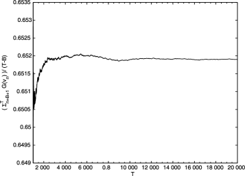
Figure 1: Convergence of empirical averages of the Gini, $B=1000$.

9 Presentation of the results

9.1 Results with the described DGP

We ran a Gibbs sampler with $T=20{,}000$ and $B=1000$. In order to diagnose convergence, we plotted the convergence of the empirical averages required for the inference (see, e.g., Figure 1). As expected, due to exponential ergodicity, convergence occurs very quickly. For such values of $T$ and $B$, burn-in only changes the very last decimals. For simplicity, for such plots, we used rough design-based variance calculations based on linearization, but approximating the complex sampling design. It is only below that we use the full procedure explained in Section 4. Since the computations in the POULPE software are extensive, we take a larger value for $B$. We do not feel that this is troublesome. Indeed, large $T$ is important for convergence of the marginals of the Gibbs sampler to the invariant probability. Once convergence is satisfactory, we compute the sample analogues (11), starting close to the steady state.

In Table 5 we give posterior predictions and confidence regions and in Figure 2 we give histograms for posterior distributions of summaries of the French wealth distribution.

Table 5: Posterior predictions and $90\%$ symmetric posterior regions, (11) is used with $B=19{,}000$ and $T=20{,}000$

Summary of the distribution	Lower bound	Prediction	Upper bound
Mean (€)	202,600	211,200	218,800
Median (€)	108,800	112,500	116,600
P99 (€)	1,507,000	1,658,000	1,815,000
P95 (€)	671,900	713,300	748,400
P90 (€)	425,800	438,500	450,000
Q3 (€)	228,300	234,000	239,600
Q1 (€)	16,000	17,200	18,500
P10 (€)	3324	3900	4459
P95/D5	5.97	6.33	6.64
P99/D5	13.30	14.71	16.17
Q3/Q1	12.71	13.72	14.50
D9/D1	94	111.2	126.4
D9/D5	3.75	3.89	4.02
Gini	0.644	0.657	0.669
Theil	0.870	0.930	0.984
Atkinson ($\varepsilon=1.5$)	0.904	0.921	0.940
Atkinson ($\varepsilon=2$)	0.974	0.983	0.993

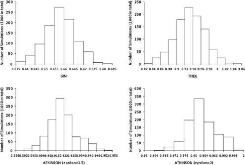
Figure 2: Posterior distribution of the Gini, Theil and Atkinson indices, full 5 components model, $T=20{,}000$ and $B=19{,}000$.

9.2 Stability of the results regarding the aggregation of wealth components

To study the relative stability of the results regarding the aggregation of wealth components, we present an alternative DGP model with fewer wealth components and thus fewer wealth categories.

Suppose we decide to group together the values of the share held of the principal residence and of the holdings in other real estate. We now work with the following components: (1) financial wealth, $\tilde{W}^{1}$; (2) wealth in real estate, $\tilde{W}^{2}$; (3) the professional wealth, $\tilde{W}^{3}$; and (4) the remainder, $\tilde{W}^{4}$. Table 6 gives details about the size of each of the $4=2^{2}$ groups. The new wealth component is homogeneous in the sense that it is investment in real estate. The choice is slightly less justifiable from a wealth accumulation perspective, as principal residence and other real estate are usually acquired one after the other. Also, the second can yield returns. As a result, it is also possible to argue that it is of a similar nature as some of the financial wealth. The lower and upper bounds for this new aggregated component were obtained by summing up respectively the lower bounds and upper bounds of $s_{2}W_{2}$ and $W_{3}$. As a result, we only have for the new component $11.9$% of point measures. For all the other components we do not have any point measures. We were no longer able to use variables on the principal residence as covariates. For example, it makes little sense to use the surface of the principal residence to predict the value of the total share in real estate. In this case, liability for the ISF is more difficult to exploit, as one is allowed to have a rebate of 20% on the value of one’s principal residence. We used rougher upper and lower bounds of taxable wealth

=300pt Component/Group 1 2 3 4 $\tilde{W}^{1}$ $\surd$ $\surd$ $\surd$ $\surd$ $\tilde{W}^{2}$ $\surd$ $\surd$ $\tilde{W}^{3}$ $\surd$ $\surd$ $\tilde{W}^{4}$ $\surd$ $\surd$ $\surd$ $\surd$ Size 1642 4600 275 3175

Table 6: Patterns of holdings

$$\tilde{W}_{k}^{1}+\tilde{W}_{k}^{2}+\mathit{ND}_{k}\min(\tilde{W}_{k}^{3},\mathit{NDED}_{\max,k})+\tilde{W}_{k}^{4}-\mathit{DEBT}_{k},$$ (12)

$$\tilde{W}_{k}^{1}+0.8\tilde{W}_{k}^{2}+\mathit{NDED}_{\min,k}-\mathit{DEBT}_{k}.$$ (13)

When a household pays the tax, (12) is greater than 720,000 €, while when it does not pay the tax, (13) is less than 720,000 €. In Table 7 we give posterior predictions and confidence regions with the three-stage model with this new DGP model. The interval estimates use calculations of the asymptotic variances of the survey sampling estimators based on the procedure presented in Section 4. This 4 components DGP yields results which are highly comparable to those obtained for the 5 components DGP studied previously.

Table 7: Posterior predictions and $90\%$ symmetric posterior regions ($T=20{,}000$, $B=19{,}000$)

Summary of the distribution	Lower bound	Prediction	Upper bound
Mean (€)	203,100	211,300	219,100
Median (€)	108,700	112,600	116,400
P99 (€)	1,498,000	1,661,200	1,822,300
P95 (€)	673,100	714,000	749,700
P90 (€)	426,300	438,800	451,000
Q3 (€)	228,800	234,100	239,900
Q1 (€)	16,020	17,210	18,470
P10 (€)	3313	3914	4506
P95/D5	5.98	6.34	6.67
P99/D5	13.19	14.74	16.33
Q3/Q1	12.67	13.59	14.51
D9/D1	94.4	111.6	128.7
D9/D5	3.76	3.89	4.03
Gini	0.644	0.658	0.670
Theil	0.872	0.931	0.989
Atkinson ($\varepsilon=1.5$)	0.904	0.921	0.940
Atkinson ($\varepsilon=2$)	0.974	0.983	0.993

10 Concluding discussion

In order to analyze the French wealth distribution based on the 2004 EP, we proposed a Bayesian hierarchical modeling. We produced point and interval estimates of summaries of a finite population distribution under random sampling, and in the presence of generalized nonrectangular censoring. The approach is flexible, as we can compute any possible such summaries (quantiles, inequality indices, etc.), and is particularly useful when the summaries are nonlinear in the input distribution. Unlike the original Bayesian multiple imputation, we do not rely on proper—that is, independent—Bayesian multiple imputations [Little and Rubin (2002); Schafer (2001)], which could be computationally intensive to obtain, nor rely on approximate formulas to combine multiple imputations. Usually official statisticians do not like to rely on models for the DGP. This does not seem feasible in the presence of interval censored data and when the sample survey estimator is “nonlinear” in the respondent’s wealth. It was, however, possible to take into account the complexity of the sample design, auxiliary information on totals through calibration, etc., using model (I). It is also possible to adopt a model-based approach and to simulate the wealth for the nonsampled households, but then the design features are not taken into account. As noted in Section 2, unit nonresponse was modeled as an extra phase, resulting in estimated weights. As it is usually done in practice, they were treated as the true inverse of the inclusion probabilities. Interval estimates are thus slightly optimistic. One way to deal with this problem is to treat the true weights as observed with error and add an extra model in the hierarchy of models. It implies to augment the state space of the Gibbs sampler presented in Section 8. We could also include uncertainty in the model choice, including, for example, the possibility of a Pareto distribution, with an additional model in the hierarchy and prior weights on each model in competition. Indeed, distributional assumptions made for the DGP are crucial especially for the wealthiest. Finally, Assumption (A), made here for the unit nonresponse, is a strong assumption that is made in most of the literature on missing data in surveys. It is possible to relax this assumption via strong parametric assumptions [Gautier (2005)]. These extensions of the methodology proposed in this article could be studied, for example, in a simpler setting.

We favored objectivity and tried to impose the minimum possible structure. For this reason, we used noninformative priors and did not impose any structure on the covariance matrices in the DGP model. A common practice is to assume diagonal covariance matrices for the residuals. This is the case when imputations, possibly multiple imputations, are done independently for each wealth component. This is very questionable, as it is not coherent with the portfolio choice theory. We feel that it imposes too much structure. The cost for this objectivity is relatively large interval estimates. We feel, though, that it is important for a national statistical office to be as objective as possible. Specification of the DGP components was taken to be the most classical lognormal one. We traded off the number of parameters for posterior regions with reasonable coverage. The model for the multivariate DGP has a reasonably small number of components and covariates for groups of small sample size. The components form homogeneous blocks in terms of population and wealth accumulation history. Observed heterogeneity is introduced through fixed effects and covariates, unobserved heterogeneity through correlations of error terms with group specific covariance matrices.

It is always useful to gather information from sources exterior to the survey. This is difficult when one is using other survey data, due to different concepts, different selection mechanisms, especially because of unit nonresponse and the different perception of surveys and different dates. Here we were able to use matched administrative data for the same year to better localize the interval censored wealth components.

Further improvement could be made for the measurement of wealth with a sampling scheme designed explicitly for the study of the wealth inequality. Because of its list sample, the SCF is probably better designed for such studies. One possibility studied for the EP is to draw households based on the wealth and property taxes (note that the notion of household based on principal residences is different from the one used for tax purposes), but it raises issues concerning tax secrecy. In any case, there are limits to a better sampling design: confidentiality, the relative coarser information for the wealthiest due to the collection of brackets, the general use of the data; as well as limits inherent to social statistics: nonresponse, biased responses, errors in recall for overview questions, misunderstanding, etc.

References

- Atkinson (1970) Atkinson, A. B. (1970). On the measurement of inequality. J. Econom. Theory 2 244–263. \MR0449508
- Caron, Deville and Sautory (1998) Caron, N., Deville, J. C. and Sautory, O. (1998). Estimation de précision de données issues d’enquêtes: document méthodologique sur le logiciel POULPE. Document de travail INSEE M9806.
- Chand and Gan (2003) Chand, H. and Gan, L. (2003). The effect of bracketing in wealth estimation. Review of Income and Wealth 49 273–287.
- Cordier and Girardot (2007) Cordier, M. and Girardot, P. (2007). Comparaison et recalage des montants de l’enquête patrimoine sur la comptabilité nationale. Document de travail INSEE F0702.
- Dell et al. (2002) Dell, F., d’Haultfœuille, X., Février, P. and Massé, E. (2002). Mise en œuvre de calcul de variance par linéarisation. Actes des Journées de Méthodologie Statistique. Available at http://jms.insee.fr/files/documents/2002/349_1- JMS2002_SESSION5_DELL-DHAULTFOEUILLE-FEVRIER-MASSE_ACTES.PDF.
- Deville and Särndal (1992) Deville, J. C. and Särndal, C. E. (1992). Calibration estimators in survey sampling. J. Amer. Statist. Assoc. 87 376–382. \MR1173804
- Deville (1999) Deville, J. C. (1999). Variance estimation for complex statistics and estimators: Linearization and residual techniques. Survey Methodol. 25 193–203.
- Foster (1983) Foster, J. E. (1983). An axiomatic characterization of the Theil measure of income inequality. J. Econom. Theory 2 244–263. \MR0720116
- Gautier (2005) Gautier, E. (2005). Eléments sur les mécanismes de sélection dans les enquêtes et sur la non-réponse non-ignorable. Actes des Journées de Méthodologie Statistique. Available at http://jms.insee.fr/files/documents/2005/445_1- JMS2005_SESSION16_GAUTIER_ACTES.PDF.
- Heeringa, Little and Raghunathan (2002) Heeringa, S. G., Little, R. J. A. and Raghunathan, T. E. (2002). Multivariate imputation of coarsened survey data on household wealth. In Survey Nonresponse (R. M. Groves et al., eds.). Wiley, Hoboken, NJ.
- Juster and Smith (1997) Juster, T. F. and Smith, J. P. (1997). Improving the quality of economic data: Lessons from the HRS and AHEAD. J. Amer. Statist. Assoc. 92 1268–1278.
- Kennickell (1998) Kennickell, A. B. (1998). Multiple imputation in the survey of consumer finances. In Proceedings of the Section on Business and Economic Statistics, 1998 Annual Meetings of the American Statistical Association, Dallas, TX. Available at http:// www.federalreserve.gov/pubs/oss/oss2/papers/impute98.pdf.
- Little and Rubin (2002) Little, R. J. A. and Rubin, D. B. (2002). Statistical Analysis with Missing Data, 2nd ed. Wiley, Hoboken, NJ. \MR1925014
- Matei and Tillé (2005) Matei, A. and Tillé, Y. (2005). Evaluation of variance approximations and estimators in maximum entropy sampling with unequal probability and fixed sample size. Journal of Official Statistics 21 543–570.
- McCulloch and Rossi (1994) McCulloch, R. and Rossi, P. E. (1994). An exact likelihood analysis of the multinomial Probit model. J. Econometrics 64 207–240. \MR1310524
- Robert (1995) Robert, C. (1995). Simulation of truncated normal variables. Statist. Comput. 5 121–125.
- Robert and Casella (2004) Robert, C. P. and Casella, G. (2004). Monte Carlo Statistical Methods, 2nd ed. Springer, New York. \MR2080278
- Roberts and Polson (1994) Roberts, G. O. and Polson, N. G. (1994). On the geometric convergence of the Gibbs sampler. J. Roy. Statist. Soc. Ser. B 56 377–384. \MR1281941
- Särndal, Swensson and Wretman (1992) Särndal, C. E., Swensson, B. and Wretman, J. H. (1992). Model Assisted Survey Sampling. Springer, New York. \MR1140409
- Schafer (2001) Schafer, J. L. (2001). Analysis of Incomplete Multivariate Data, 2nd ed. Chapman and Hall, London. \MR1692799
- Shao (1994) Shao, J. (1994). -statistics in complex survey problems. Ann. Statist. 22 946–967. \MR1292550
- Theil (1967) Theil, H. (1967). Economics and Information Theory. North-Holland, Amsterdam.