Response-adaptive dose-finding under model uncertainty

Abstract

Dose-finding studies are frequently conducted to evaluate the effect of different doses or concentration levels of a compound on a response of interest. Applications include the investigation of a new medicinal drug, a herbicide or fertilizer, a molecular entity, an environmental toxin, or an industrial chemical. In pharmaceutical drug development, dose-finding studies are of critical importance because of regulatory requirements that marketed doses are safe and provide clinically relevant efficacy. Motivated by a dose-finding study in moderate persistent asthma, we propose response-adaptive designs addressing two major challenges in dose-finding studies: uncertainty about the dose-response models and large variability in parameter estimates. To allocate new cohorts of patients in an ongoing study, we use optimal designs that are robust under model uncertainty. In addition, we use a Bayesian shrinkage approach to stabilize the parameter estimates over the successive interim analyses used in the adaptations. This approach allows us to calculate updated parameter estimates and model probabilities that can then be used to calculate the optimal design for subsequent cohorts. The resulting designs are hence robust with respect to model misspecification and additionally can efficiently adapt to the information accrued in an ongoing study. We focus on adaptive designs for estimating the minimum effective dose, although alternative optimality criteria or mixtures thereof could be used, enabling the design to address multiple objectives. In an extensive simulation study, we investigate the operating characteristics of the proposed methods under a variety of scenarios discussed by the clinical team to design the aforementioned clinical study.

, ,
and   Bjorn Bornkamp, Frank Bretz, Holger Dette, Jose Pinheiro a1Supported in part by the Collaborative Research Center “Statistical modeling of nonlinear dynamic processes” (SFB 823) of the German Research Foundation (DFG).

1 Introduction

Dose-finding studies have several challenges in common. First, they usually address two distinct objectives, which lead to different requirements on the study design [Ruberg (1995), Bretz et al. (2008)]: (i) assessing evidence of a drug effect, and (ii) estimating relevant target doses. Second, the form of the dose-response relationship is unknown prior to the study, leading to model uncertainty. This problem is often underestimated, although ignoring model uncertainty can lead to highly undesirable effects [Chatfield (1995), Draper (1995), Hjorth (1994)]. Third, data from dose-finding studies are usually highly variable. This issue is of particular importance in pharmaceutical drug development, because sample sizes are kept to a minimum for ethical and financial reasons. It is therefore critical to develop efficient dose-finding study designs that use the limited information as efficiently as possible, while addressing the above challenges.

Many approaches have been proposed in the optimal design literature to distribute patients efficiently with regard to given study objectives; see Wu (1988), Fedorov and Leonov (2001) and King and Wong (2004), among many others. However, most of this work has concentrated on an assumed fixed dose-response model. As there is typically considerable model uncertainty at the planning stage of a dose-response study, these methods have limited practical use. Based on concepts introduced by Läuter (1974) [see also Cook and Wong (1994), Zhu and Wong (2000, 2001), Biedermann, Dette and Pepelyshev (2006)], Dette et al. (2008) investigated model-robust designs that provide efficient target dose estimates for a set of candidate dose-response models, rather than for a single dose-response model. However, their designs require knowledge about the unknown parameters associated with the anticipated dose-response models as well as the prespecification of model probabilities.

A natural remedy is to investigate response-adaptive designs (adaptive designs, in short) with several cohorts of subjects. After each stage the accumulated information of the ongoing study is used to update the initial information of the underlying model parameters and model probabilities, which in turn is used to calculate the design for the subsequent stage(s). Several adaptive designs have been developed for this problem; see, for example, Miller, Guilbaud and Dette (2007) and Dragalin, Hsuan and Padmanabhan (2007) for recent approaches using optimal design theory, or Zhou et al. (2003), Müller et al. (2006), and Wathen and Thall (2008) for recent Bayesian adaptive designs. Dragalin et al. (2010) performed an extensive simulation study that compared five different adaptive dose-finding methods.

In this paper we propose adaptive designs addressing the three major challenges described above: multiple study objectives, model uncertainty and large variability in the data. For this purpose we use the model-robust designs proposed by Dette et al. (2008) together with a Bayesian shrinkage approach to stabilize the parameter estimates, especially in the early part of a study. This allows one to calculate parameter estimates as well as model probabilities that can then be used to calculate model-robust designs for the subsequent stage(s) of the study. The resulting designs are robust with respect to model misspecification and additionally adapt to the continuously accrued information in an ongoing study. We focus on adaptive designs for estimating the minimum effective dose (MED), that is, the smallest dose achieving a clinically relevant benefit over the placebo response. However, alternative optimality criteria or mixtures of optimality criteria could be used, enabling the design to address multiple objectives.

2 Asthma dose-finding study

The research for this article was motivated by a Phase II dose-finding study for the development of a new pharmaceutical compound in asthma. This was a multi-center, randomized, double-blind, placebo controlled, parallel group study in patients with moderate persistent asthma, who were randomized to one of seven active dose levels or placebo. The primary endpoint was change from baseline in a lung function parameter (forced expiratory volume in 1 second, $FEV_{1}$) after 28 days of administration, scaled such that larger values indicated a better outcome. The objective of the trial was to evaluate the dose effects over placebo for the primary endpoint and to assess whether there was any evidence of a drug effect. Once such a dose-response signal had been detected, one would subsequently estimate relevant target doses, where the primary focus was on estimating the MED.

Based on discussions with the clinical team, a homoscedastic normal model was assumed for the primary endpoint with a standard deviation of 350 ml, a placebo effect of 100 ml and a maximum treatment effect of 300 ml within the dose range [0, 50] under investigation. The available doses were 0 ($={}$placebo), 0.5, 1.0, 2.5, 5, 10, 20 and 50. The clinically relevant benefit over the placebo effect was set to 200 ml. That is, an increase in treatment effect of less than 200 ml over the observed placebo response was considered to be clinically irrelevant. Furthermore, all dose levels within the investigated dose range were considered safe based on previous studies, so that efficacy was of primary interest.

Because this study was conducted early in the drug development program, limited information about the dose-response shape was available at the planning stage. A set of candidate dose-response models was derived before starting the study; see Table 1 and Figure 1 for the full model specifications (including a preliminary specification of the model parameters). An increase of the dose-response curve in the lower part of the investigated dose range was considered likely, so two concave increasing models (Emax₁, Emax₂) were included in the model set. In addition, $S$-shaped (Logistic₁), unimodal (Beta) and convex (Logistic₂) models were included in the candidate model set to robustify the statistical analysis with respect to model uncertainty. We refer to Pinheiro, Bornkamp and Bretz (2006) for details on the use of candidate models in dose-response studies and the elicitation of best guesses for the model parameters.

Table 1: Candidate dose response models as a function of dose $d$, where $B({a},{b})=({a}+{b})^{{a}+{b}}/({a}^{a}{b}^{b})$

Model	Full model specification	Model parameters	True MED
Beta	$\theta_{0}+\theta_{1}B(\theta_{2},\theta_{3})(d/60)^{\theta_{2}}(1-d/60)^{\theta_{3}}$	(100, 300, 0.43, 0.6)	$5.21$
Emax1	$\theta_{0}+\theta_{1}d/(\theta_{2}+d)$	(100, 420, 20)	$18.18$
Emax2	$\theta_{0}+\theta_{1}d/(\theta_{2}+d)$	(100, 330, 5)	$7.69$
Logistic1	$\theta_{0}+\theta_{1}/\{1+\exp[(\theta_{2}-d)/\theta_{3}]\}$	(98, 302, 17.5, 3.3)	$19.82$
Logistic2	$\theta_{0}+\theta_{1}/\{1+\exp[(\theta_{2}-d)/\theta_{3}]\}$	(92, 615, 50, 11.5)	$42.28$

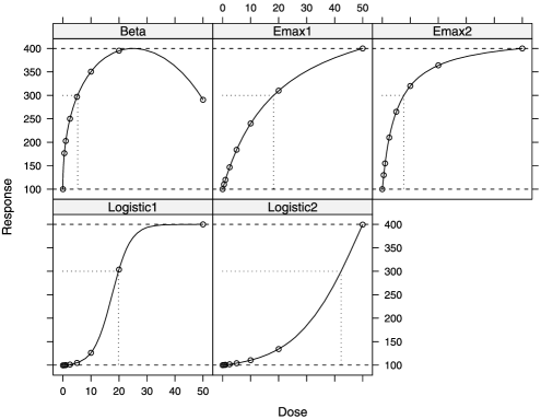
Figure 1: Graphical display of the dose-response models in Table 1. Open dots denote the potential responses at the seven active dose levels and placebo available in the study. Dotted horizontal lines indicate the clinical relevance threshold on top of placebo response and dotted vertical lines the resulting MED.

Given the information and constraints above, the clinical team was faced at the planning stage with several remaining key questions on the study design: [(B)]

Should an adaptive design be employed at all or would a nonadaptive design be sufficient?

If the decision was to employ an adaptive design, how many interim analyses should be conducted?

How many dose levels should be included in the study, that is, are all seven active dose levels from above needed?

If not all active dose levels were needed, which of them should then be investigated? In addition to these statistical questions, many further considerations were discussed by the clinical team: adaptive designs require more logistical effort to set up the repeated data collection and cleaning/analysis processes than nonadaptive designs; including all seven active doses in the study would pose serious challenges to the drug manufacturing and supply departments, especially if the allocation changed during the study course; and how to ensure trial integrity and validity. In the following we focus on the statistical questions and describe the proposed methodology for the study.

3 Methodology

Assume $k$ distinct dose levels $d_{1},\ldots,d_{k}$, where $d_{1}=0$ denotes placebo. Let $n_{i}$ patients be allocated to dose $d_{i}$ and $N=\sum_{i=1}^{k}n_{i}$. The vector of allocation weights is denoted by $\mathbf{w}=(w_{1},\ldots,w_{k})^{\prime}$, where $w_{i}=n_{i}/N$. Let further $Y_{ij}\sim N(f(d_{i},\bolds\theta),\sigma^{2})$ denote the observation of patient $j=1,\ldots,n_{i}$ at dose $d_{i},i=1,\ldots,k$, where the dose-response model $f(\cdot)$ is parameterized through the parameter vector $\bolds\theta$ and $N(\mu,\sigma^{2})$ denotes the normal distribution with mean $\mu$ and variance $\sigma^{2}$.

Most dose-response models used in practice, including those in Table 1, can be decomposed as

$$f(d,\bolds\theta)=\theta_{0}+\theta_{1}f^{0}(d,\bolds\theta^{0}),$$ (1)

where $\bolds\theta=(\theta_{0},\theta_{1},{\bolds\theta^{0}}^{\prime})^{\prime}=(\theta_{0},\ldots,\theta_{p})^{\prime}$. The parameters $\bolds\theta^{*}=(\theta_{0},\theta_{1})^{\prime}$ enter the model function $f$ linearly and determine its location and scale, while $f^{0}$ is typically a nonlinear function that determines the shape of the model function $f$ through the parameters $\bolds\theta^{0}$.

The minimum effective dose producing a clinically relevant effect $\Delta$ over the placebo response is defined as

$$\mathrm{MED}=\min_{d\in(d_{1},d_{k}]}\{f(d,\bolds\theta)>f(d_{1},\bolds\theta)+\Delta\},$$ (2)

where we assume that a beneficial effect is associated with larger values of the response variable. Note that the MED may not exist, as no dose in $(d_{1},d_{k}]$ may produce an improvement of $\Delta$ compared with placebo.

3.1 Robust designs for MED estimation

Given a function $f^{0}$, it follows from (2) that the MED (provided it exists) is a solution to

$$\theta_{0}+\theta_{1}f^{0}(0,\bolds\theta^{0})+\Delta=\theta_{0}+\theta_{1}f^{0}(\mathrm{MED},\bolds\theta^{0}).$$ (3)

Consequently, $\mathrm{MED}=b(\bolds\theta)=h^{0}(f^{0}(\mathrm{0},\bolds\theta^{0})+\Delta/\theta_{1})$, where $h^{0}(x)=\inf\{z|\break f^{0}(z)\geq x\}$ denotes the (generalized) inverse of the function $f^{0}$ with respect to the variable $d$. Standard asymptotic theory for nonlinear models [Seber and Wild (1989)] yields that the maximum likelihood (ML) estimate $\widehat{\bolds\theta}$ is approximately multivariate normal distributed with mean vector $\bolds\theta$ and covariance matrix $\frac{\sigma^{2}}{N}\mathbf{M}^{-1}(\bolds\theta,\mathbf{w}),$ where $\mathbf{M}(\bolds\theta,\mathbf{w})=\sum_{i=1}^{k}w_{i}g(d_{i},\bolds\theta)g(d_{i},\bolds\theta)^{\prime}$ denotes the information matrix and $g(d,\bolds\theta)=\frac{\partial f(d,\bolds\theta)}{\partial\bolds\theta}$ the gradient of the dose-response model $f$ with respect to $\bolds\theta$. It follows from the $\delta$-method [see van der Vaart (1998)] that the $\mathrm{MED}$ estimator based on $\widehat{\bolds\theta}$, $\widehat{\mathrm{MED}}=b(\widehat{\bolds\theta})$, is asymptotically normally distributed with mean $b(\bolds\theta)$ and variance $V(\bolds\theta,\mathbf{w})=\frac{\sigma^{2}}{N}\bolds\nabla b(\bolds\theta)^{\prime}\mathbf{M}^{-1}(\bolds\theta,\mathbf{w})\bolds\nabla b(\bolds\theta)$, where $\bolds\nabla b(\bolds\theta)=\frac{\partial b(\bolds\theta)}{\partial\bolds\theta}$. Hence, minimizing $V(\bolds\theta,\mathbf{w})$ with respect to $\mathbf{w}\in\mathbb{S}^{k}=\{\mathbf{w}|\sum_{i=1}^{k}w_{i}=1,\mathbf{w}\geq 0\}$ results in optimal designs that minimize the approximate variance of $\widehat{\mathrm{MED}}$. This design criterion has also an appealing decision theoretic justification: The asymptotic normal distribution of $\widehat{\mathrm{MED}}$ approximates the posterior distribution of the $\mathrm{MED}$ in a Bayesian model framework. Hence, minimizing the log-variance of $\widehat{\mathrm{MED}}$ is equivalent to minimizing the (approximate) Shannon entropy of the posterior distribution of the $\mathrm{MED}$ [Chaloner and Verdinelli (1995)].

In principle, the above optimization could be done with respect to the number and choice of doses and their corresponding allocation ratios [Dette et al. (2008)], but, in practice, manufacturing constraints often determine the available doses, as it was the case in the asthma study from Section 2. In the following we thus restrict the optimization to the weights $\mathbf{w}$ for prespecified doses $d_{1},\ldots,d_{k}$.

The true dose-response function $f$ is unknown and optimal designs are typically not robust with respect to model misspecification [Dette et al. (2008)]. In the following we assume a set of $M$ candidate models $f_{m}(d,\bolds\theta_{m})=\theta_{0m}+\theta_{1m}f_{m}^{0}(d,\bolds\theta^{0}_{m})$, $m=1,\ldots,M$, such as those described in Table 1. We “integrate” the design criterion conditional on model $m$ with respect to the model probabilities $\alpha_{m}$. Hence, using the design criterion $\sum_{m=1}^{M}\alpha_{m}\log(V_{m}(\bolds\theta_{m},\mathbf{w}))$ or, equivalently,

$$\Psi(\mathbf{w})=\prod^{M}_{m=1}(V_{m}(\bolds\theta_{m},\mathbf{w}))^{\alpha_{m}}$$ (4)

leads to designs that are robust with respect to model misspecification, where $V_{m}(\bolds\theta_{m},\mathbf{w})$ denotes the variance of the estimate for the MED in the $m$th model $(m=1,\ldots,M)$. Note that because of taking logarithms above, there is no need to standardize the individual model variances. Otherwise this would be necessary to avoid that some models dominate the design criterion [the $V_{m}(\bolds\theta_{m},\mathbf{w})$ can be quite model dependent and differing in size]. However, the numerical calculation of robust designs using the criterion (4) requires the knowledge of $\bolds\theta_{m}$ and $\alpha_{m},m=1,\ldots,M$. In the following sections we describe how the initial best parameter guesses can be updated during an ongoing study such that subsequent stages can be redesigned based on the updated estimates for $\bolds\theta_{m}$ and $\alpha_{m},m=1,\ldots,M$; see Section 3.3 for a description of the complete procedure in an algorithmic form.

3.2 Updating of model parameters and weights

Reliably estimating the parameters $\bolds\theta_{1},\ldots,\bolds\theta_{M}$ is a challenging problem, particularly in early stages of a study. ML estimates for these parameters are typically highly variable, and may even not exist without imposing bounds on the parameter space. One way of stabilizing estimates is to use a shrinkage approach based on, for example, penalized maximum likelihood or maximum a-posteriori (MAP) estimates. Here, one optimizes the log-likelihood function plus a term which determines the prior plausibility of the parameters (the log prior distribution). The estimate is then a compromise between the information contained in data and the prior distribution. This stabilizes the estimates in early stages due to the shrinkage toward a priori reasonable values. In later stages the shrinkage effect decreases because the log prior remains constant while the log likelihood receives more weight with increasing sample sizes. If a completely flat prior distribution is used, standard ML and MAP estimation coincide, so that using nonuniform priors is desirable. We discuss the choice of nonuniform priors in more detail further below.

Apart from stable parameter estimates $\bolds\theta_{1},\ldots,\bolds\theta_{M}$ for the dose-response models, one needs to update the model probabilities $\alpha_{1},\ldots,\alpha_{M}$ at an interim analysis. We propose using a probability distribution over the different dose-response models and evaluating the posterior probabilities for each model after having observed the data; see, for example, Kass and Raftery (1995) for a detailed description of posterior probabilities and Bayes factors. These posterior model probabilities can then be used in the design criterion (4). A computationally efficient approach to approximate the posterior model probabilities is the Bayesian information criterion (BIC). However, previous simulation studies in the context of dose-finding studies showed that the BIC approximation frequently favors too simplistic models for realistic variances and sample sizes [see Bornkamp (2006)]. Other approximate methods, such as fractional Bayes factors, or intrinsic Bayes factors [see O’Hagan (1995) or Berger and Pericchi (1996)], either depend on arbitrary tuning parameter values or are computationally prohibitive. Thus, for each model we will use the exact posterior probabilities resulting from the prior distributions assumed for the MAP estimation. In our case, these probabilities can be calculated using efficient numerical quadrature without the need to resort to computationally expensive Markov chain Monte Carlo techniques. In the remainder of this section we provide details on the prior elicitation and the calculation of posterior probabilities.

3.2.1 Selection of prior distributions for $\bolds\theta_{m}$

We utilize the factorization in (1) to derive a prior distribution for $(\theta_{0m},\theta_{1m},\bolds\theta^{0}_{m},\sigma^{2})$. If $\bolds\theta^{0}_{m}$ were known, the nonlinear models would reduce to a linear model. It is therefore reasonable to use for a given $\bolds\theta^{0}_{m}$ the conditionally conjugate normal-inverse gamma (NIG) distribution

$$p(\bolds\theta^{*}_{m},\sigma^{2}|\bolds\theta^{0}_{m})\propto(\sigma^{2})^{-(\nu+4)/2}\exp[-\{(\bolds\theta^{*}_{m}-\bolds\mu)^{\prime}{\mathbf{V}}^{-1}(\bolds\theta^{*}_{m}-\bolds\mu)+a\}/(2\sigma^{2})]$$

for $(\bolds\theta^{*}_{m},\sigma^{2})$ [see O’Hagan and Forster (2004)], where the parameter $\bolds\theta^{*}$ is defined after equation (1), $a,\nu>0$, $\bolds\mu\in\mathbb{R}^{2}$ and $\mathbf{V}\in\mathbb{R}^{2\times 2}$ denotes a positive definite matrix. The NIG distribution marginally induces a bivariate $t$-distribution for $\bolds\theta^{*}_{m}$ with $\nu$ degrees of freedom, finite mean $\bolds\mu$ and covariance matrix $a/(\nu-2)\mathbf{V}$, provided that $\nu>2$. The marginal prior distribution for $\sigma^{2}$ is given by an IG distribution with mode $a/(\nu+2)$, mean $a/(\nu-2)$ and variance $2a^{2}/\{(\nu-2)^{2}(\nu-4)\}$. It has a finite mean when $\nu>2$ and a finite variance when $\nu>4$.

To set up the NIG distribution for $(\bolds\theta^{*}_{m},\sigma^{2})$, one can employ available information about the placebo effect, the maximum treatment effect and the standard deviation. For example, one can choose the marginal bivariate $t$-distribution for $\bolds\theta^{*}_{m}$ (conditional on $\bolds\theta^{0}_{m}$) such that the desired mean and covariance are achieved for the placebo effect and the maximum effect of the underlying dose-response model. When the linear parameters $\bolds\theta^{*}_{m}$ cannot be interpreted as placebo and maximum effect, one can use a suitable transformation to achieve the desired moments. Then, one can adjust $a$ and $d$ so that the marginal distribution of $\sigma^{2}$ achieves the desired mode. An attractive choice is to use $\nu=4$, leading to a prior with infinite variance for $\sigma^{2}$ and a heavy tailed marginal prior for $\bolds\theta^{*}_{m}$.

Figure 2: Beta priors on $[0.5,75]$ with mode 20 and different $S$ values.

For the nonlinear parameters $\bolds\theta^{0}_{m}$, we propose selecting suitable bounds for the parameters and then eliciting a bounded prior distribution. This is typically not difficult, as the interpretation of the nonlinear parameters is straightforward, and excessively large parameter values usually correspond to a priori unlikely model shapes. We propose using a scaled beta distribution $B(\alpha,\beta)$ with mode equal to the initial parameter guesses. The curvature of the prior determines the amount of shrinkage that one is willing to employ for the MAP estimates. In the simulations we used the sum $S=\alpha+\beta$ as a measure of curvature with $S>2$ to ensure unimodality of the beta distribution. Note that already relatively small values of $S$, such as $S=10$ or $S=20$, lead to strong shrinkage effects; see Figure 2 for an illustration of the $\theta_{2}$ parameter in the Emax₁ model, where the initial parameter guess is 20. For dose-response models with more than one nonlinear parameter, we repeat this procedure for all parameters and assume independence among them.

For selecting prior model probabilities, it is convenient to use a uniform distribution across the models unless some models are deemed a priori more plausible than others.

3.2.2 Calculation of posterior probabilities

Let $\mathbf{y}$ denote the data available at an interim analysis and $p({\mathbf{y}}|\bolds\theta_{m},m)$ the likelihood under model $m$ with corresponding prior distribution $p(\bolds\theta_{m}|m)$ and prior model probability $p(m)$. Then the marginal likelihood is given by

$$p(m|{\mathbf{y}}) \propto p(m)\int p({\mathbf{y}}|\bolds\theta_{m},\sigma^{2},m)p(\bolds\theta_{m},\sigma^{2}|m)\,d(\bolds\theta_{m},\sigma^{2})$$

$$\propto p(m)\int\int p({\mathbf{y}}|\bolds\theta_{m},\sigma^{2},m)p(\bolds\theta^{*}_{m},\sigma^{2}|\bolds\theta^{0}_{m},m)\,d(\bolds\theta^{*}_{m},\sigma^{2})p(\bolds\theta^{0}_{m}|m)\,d\bolds\theta^{0}_{m}.$$

The inner integral in the last equation is the product of a likelihood and a conjugate prior distribution. One can hence reduce the integration to

$$p(m|{\mathbf{y}})\propto p(m)\int p({\mathbf{y}}|\bolds\theta^{0}_{m},m)p(\bolds\theta^{0}_{m}|m)\,d\bolds\theta^{0}_{m},$$ (5)

where $p({\mathbf{y}}|\bolds\theta^{0}_{m},m)$ now denotes the integrated likelihood. In our applications, the integral (5) is one- or two-dimensional over a bounded region and hence straightforward to calculate numerically. This allows us to calculate the marginal likelihoods efficiently, without resorting to Markov chain Monte Carlo calculations; see Section 3.4 for details. The posterior model probabilities $p(m|{\mathbf{y}})$ can be obtained by normalizing the marginal likelihoods (multiplied by the prior model probabilities).

We use the maximum $\tilde{\bolds\theta}^{0}_{m}$ of the marginal posterior $p({\mathbf{y}}|\bolds\theta^{0}_{m},m)p(\bolds\theta^{0}_{m}|m)$ as an estimate of $\bolds\theta^{0}_{m}$. Conditional on this value, we use the maximum $\tilde{\bolds\theta}^{*}_{m}$ of $p(\bolds\theta^{*}_{m}|\tilde{\bolds\theta}^{0}_{m},\mathbf{y},m)$ as an estimate for $\bolds\theta^{*}_{m}$. Therefore, the overall estimate of the parameter $\bolds\theta_{m}$ is given by $\tilde{\bolds\theta}_{m}=(\tilde{\bolds\theta}^{*}_{m},\tilde{\bolds\theta}^{0}_{m})$. This is a slight variation of the MAP approach described above, but reduces further the computational effort, as it reuses the calculations from the integration to obtain the marginal likelihoods.

3.3 Main algorithm

We now summarize the complete response-adaptive dose-finding design in algorithmic form.

Before trial start: [(5)]

Select a starting design using either a balanced allocation across the available doses or an unbalanced allocation based on optimal design considerations.

Select candidate dose-response models $f_{m}(d,\bolds\theta_{m})$.

Conditional on $\bolds\theta_{m}^{0}$, calculate a NIG prior distribution for ($\bolds\theta^{*}_{m}$, $\sigma^{2}$) based on “best guesses” for the placebo effect, the maximum treatment effect and $\sigma^{2}$ (together with suitable variability assumptions for both parameters).

Choose “best guesses” for the nonlinear parameters $\bolds\theta^{0}_{m}$ and select the parameter $S$.

Choose prior model probabilities $p(m)$ for the different dose-response functions.

At interim analysis: [(3)]

Calculate posterior model probabilities

$$p(m|{\mathbf{y}})\propto p(m)\int p({\mathbf{y}}|\bolds\theta_{m},m)p(\bolds\theta_{m}|m)\,d\bolds\theta_{m}.$$ (6)

Exploiting the conjugacy properties of the NIG distribution, this reduces to one- or two-dimensional integrals; see Section 3.4 for computational details.

For each dose-response model, estimate ${\bolds\theta}_{m}$ by using the maximum of $p({\mathbf{y}}|\bolds\theta^{0}_{m},m)p(\bolds\theta^{0}_{m}|m)$, where the abscissas calculated in step 1 can be reused. Conditional on this value, use the maximum of $p(\bolds\theta^{*}_{m}|\tilde{\bolds\theta}^{0}_{m},\mathbf{y},m)$ as an estimate for $\bolds\theta^{*}_{m}$ to obtain $\tilde{\bolds\theta}_{m}$

Plug the obtained parameter estimates $\tilde{\bolds\theta}_{m}$ into (4) and set $\alpha_{m}=p(m|{\mathbf{y}})$. Then, minimize with respect to $\mathbf{w}\in\mathcal{S}$, where $\mathcal{S}=\{\mathbf{w}\in\mathbb{S}^{k}|\mathbf{w}=(\mathbf{n}_{\mathrm{old}}+N_{\mathrm{next}}\mathbf{w}_{\mathrm{next}})(N_{\mathrm{old}}+N_{\mathrm{next}})^{-1},\mathbf{w}_{\mathrm{next}}\in\mathbb{S}^{k}\}$. Here, $\mathbf{n}_{\mathrm{old}}$ denotes the vector of sample sizes per dose and $N_{\mathrm{old}}$ the total sample size until the current interim analysis. Further, $N_{\mathrm{next}}$ denotes the sample size and ${\mathbf{w}}_{\mathrm{next}}\in\mathbb{S}^{k}$ the design weights for the next cohort of patients. We therefore optimize the design for the next stage taking into account the patient allocation until the current interim analysis; see Section 3.4 for computational details.

Allocate the next cohort of patients according to $\mathbf{w}_{\mathrm{next}}$ by applying an appropriate rounding technique, such as described in Pukelsheim (1993), Chapter 12.

Note that the Bayesian approach is used here for design adaptation purposes. The final analysis may or may not be done using a fully Bayesian approach. The development of the Bayesian design methodology above is motivated by the MCP-Mod methodology described in Bretz, Pinheiro and Branson (2005) to address model uncertainty. This method requires prior estimates for the placebo effect, the maximum treatment effect, and $\sigma^{2}$ at the design stage and “best guesses” of the nonlinear parameters $\bolds\theta^{0}_{m}$ for the analysis. The additional information needed to set up the above adaptive design procedure is hence minimal. Obviously, any other strategy that allows one to use a set of candidate dose-response models might also be used for the final analysis.

3.4 Technical details

In this section we provide further details of the algorithm presented above.

For the calculation of the one- and two-dimensional integrals in (5) we used quasi-uniformly distributed point sets based on good lattice points $\mathbf{u}_{1},\ldots,\mathbf{u}_{n}$, where $\mathbf{u}_{i}\in[0,1]^{d}$ and $d$ is the dimension of $\bolds\theta_{m}^{0}$; see Fang and Wang (1994) for details on the construction of such integration grids. Let $\pi(\bolds\theta_{m}^{0}|y)=p(\mathbf{y}|\bolds\theta_{m}^{0},m)\times p(\bolds\theta^{0}_{m}|m)$ denote the integrand from (5) and let $\mathbf{b}_{l}$ and $\mathbf{b}_{u}$ denote the vector of lower and upper bounds for $\bolds\theta_{m}^{0}$. One first transforms the good lattice points to obtain $\mathbf{u}_{i}^{*}=\mathbf{u}_{i}(\mathbf{b}_{u}-\mathbf{b}_{l})+\mathbf{b}_{l}$ for $i=1,\ldots,n$, and then approximates the integral (5) by $\prod_{j=1}^{d}(b_{uj}-b_{lj})\sum_{i=1}^{n}\pi(\mathbf{u}^{*}_{i}|y)/n$. This approach also allows one to calculate the approximate maximum in the subsequent optimization step by using the grid point $\mathbf{u}^{*}_{i}$ corresponding to $\max_{i}\pi(\mathbf{u}^{*}_{i}|y)$. We found that using a grid of size 100 in the one-dimensional case and the good lattice point set of size 1597 in the two-dimensional case [Fang and Wang (1994)] provide sufficiently reliable and computationally efficient results (both for integration and optimization).

The optimization in (4) is a constrained optimization problem because the weights $\mathbf{w}_{\mathrm{next}}$ lie in the ($k-1$)-dimensional probability simplex. A simple but efficient approach to perform the optimization is to use a mapping $\mathbb{R}^{k-1}\mapsto\mathbb{S}^{k}$ and then to employ a standard unconstrained optimizer, as described in Atkinson, Donev and Tobias (2007), page 131. To account for the already allocated patients until an interim analysis, one can optimize $\Psi(\frac{\mathbf{n}_{\mathrm{old}}+N_{\mathrm{next}}\mathbf{w}_{\mathrm{next}}}{N_{\mathrm{old}}+N_{\mathrm{next}}})$ with respect to $\mathbf{w}_{\mathrm{next}}\in\mathbb{S}^{k}$. Due to potential multiple optima in the design surface, one cannot be sure whether indeed an optimal design has been found by the optimizer. We thus propose using lower bounds of the resulting relative efficiencies based on the underlying geometry of the optimization problem.

To be precise, suppose that the vector ${\mathbf{w}}^{*}$ has been found by the optimizer. The following result gives a lower bound on $r({\mathbf{w}}^{*})=\frac{\Psi(\mathbf{w}_{\mathrm{opt}})}{\Psi({\mathbf{w}}^{*})}\in[0,1]$, where $\mathbf{w}_{\mathrm{opt}}$ is the (unknown) true optimal design at the end of the next stage, accounting for the patients allocated until the current interim analysis. A proof of the result is given in the Appendix.

Theorem 3.1

A design $\mathbf{w}$ with $c_{m}(\bolds\theta_{m})=\bolds\nabla b_{m}(\bolds\theta_{m})\in\operatorname{Range}(\mathbf{M}_{m}(\bolds\theta_{m},\break\mathbf{w}))$, $m=1,\ldots,M$, minimizes $\Psi(\mathbf{w})$ with respect to $\mathbf{w}_{\mathrm{next}}$, where $\mathbf{w}=\break\frac{N_{\mathrm{old}}+N_{\mathrm{next}}\mathbf{w}_{\mathrm{next}}}{N_{\mathrm{old}}+N_{\mathrm{next}}}$, if and only if there exist generalized inverses $\mathbf{G}_{1},\ldots,\mathbf{G}_{m}$ of $\mathbf{M}_{m}(\bolds\theta_{m},\mathbf{w})$, such that the inequality

$$h(d,\mathbf{w})\!=\!\frac{\sum_{m=1}^{M}\alpha_{m}{(g_{m}^{T}(d,\bolds\theta_{m})\mathbf{G}_{m}c_{m}(\bolds\theta_{m}))^{2}/c_{m}^{T}(\bolds\theta_{m})\mathbf{G}_{m}c_{m}(\bolds\theta_{m})}}{\sum_{m=1}^{M}\alpha_{m}{c_{m}(\bolds\theta_{m})\mathbf{G}_{m}^{T}\mathbf{M}_{m}(\bolds\theta_{m},\mathbf{w}_{\mathrm{next}})\mathbf{G}_{m}c_{m}(\bolds\theta_{m})/c_{m}^{T}(\bolds\theta)\mathbf{G}_{m}c_{m}(\bolds\theta)}}\!\leq\!1$$

is satisfied for all $d\in\{d_{1},\ldots,d_{k}\}$. Moreover, the efficiency of any design $\mathbf{w}$ can be bounded from below by

$$r({\mathbf{w}})\geq\frac{1}{k^{*}(\mathbf{w},\gamma)}\geq\frac{1}{h^{*}(\mathbf{w})},$$ (7)

where $\gamma=\frac{N_{\mathrm{old}}}{N_{\mathrm{old}}+N_{\mathrm{next}}}$, $h^{*}(\mathbf{w})=\min_{{\mathbf{G}_{1},\ldots,\mathbf{G}_{m}}}\max_{d\in\{d_{1},\ldots,d_{k}\}}h(d,\mathbf{w})$,

$$k^{*}(\mathbf{w},\gamma) = \Biggl{[}1+(1-\gamma)\min_{\mathbf{G}_{1},\ldots,\mathbf{G}_{m}}\max_{\mathbf{v}\in\mathbb{S}^{k}}\sum^{M}_{m=1}\alpha_{m}c^{T}_{m}(\bolds\theta_{m})\mathbf{G}^{T}_{m}$$

$$\hphantom{\biggl{[}1+(1-\gamma)\min_{\mathbf{G}_{1},\ldots,\mathbf{G}_{m}}\max_{\mathbf{v}\in\mathbb{S}^{k}}\sum^{M}_{m=1}}{}\times\bigl{(}\mathbf{M}_{m}(\bolds\theta_{m},\mathbf{v})-\mathbf{M}_{m}(\bolds\theta_{m},\mathbf{w}_{\mathrm{next}})\bigr{)}$$

$$\hphantom{\biggl{[}1+(1-\gamma)\min_{\mathbf{G}_{1},\ldots,\mathbf{G}_{m}}\max_{\mathbf{v}\in\mathbb{S}^{k}}\sum^{M}_{m=1}}{}\times\mathbf{G}_{m}c_{m}(\bolds\theta)/(c^{T}_{m}(\bolds\theta_{m})\mathbf{G}_{m}c_{m}(\bolds\theta_{m}))\Biggr{]}^{-1}\!,$$

and the minimum is taken over all generalized inverses $\mathbf{G}_{1},\ldots,\mathbf{G}_{m}$ of the matrices $\mathbf{M}_{1}(\bolds\theta_{1},\mathbf{w}),\ldots,\mathbf{M}_{M}(\bolds\theta_{M},\mathbf{w})$.

When the matrices $\mathbf{M}_{1}(\bolds\theta_{1},\mathbf{w}),\ldots,\mathbf{M}_{M}(\bolds\theta_{M},\mathbf{w})$ are invertible, $h^{*}(\mathbf{w})$ is just the maximum of $h(d,\mathbf{w})$ over the $k$ doses and straightforward to calculate [and so is the lower bound on $r(\mathbf{w})$]. This lower bound is useful in several respects: we do not need to know the actual optimal design $\mathbf{w}_{\mathrm{opt}}$ in order to calculate the lower bound. If the lower bound for our calculated design $\mathbf{w}^{*}$ is equal to 1, we know that $\mathbf{w}^{*}$ is the optimal design. Otherwise, we have a conservative estimate on how much percent off one would be when using $\mathbf{w}$. The bound based on $k^{*}(\mathbf{w},\gamma)$ is sharper, however harder to implement.

If one does not use a fully Bayesian approach for the final analysis, one typically has to fit nonlinear regression models to the data. When there are only few doses available, as it is often the case in drug development practice, calculating the ML estimate may be difficult. One way to simplify the problem is by exploiting the fact that $\theta_{0}$ and $\theta_{1}$ enter the model function linearly in (1). We thus apply the nonlinear optimization only on the nonlinear parameters $\bolds\theta^{0}_{m}$, similar in spirit to Golub and Pereyra (2003). Using the Frisch–Waugh–Lovell theorem [Baltagi (2008), Chapter 7], we can recalculate the residual sum of squares efficiently, without the need to solve the full least squares problems in each iteration of the nonlinear optimization (this effect becomes even more important when there are additional linear covariates in the model equation, such as gender, baseline values, etc.). In addition, we impose bounds on the nonlinear parameters $\bolds\theta^{0}_{m}$ to guarantee the existence of the least squares estimate [Seber and Wild (1989), Chapter 12]. As mentioned in Section 3.2.1, such bounds are not a severe restriction in practice and ensure that the optimization problem is well posed.

4 Asthma study revisited

In this section we revisit the asthma case study from Section 2 and address the four open design questions using the proposed methodology from Section 3. To this end, we investigated in an extensive simulation study the operating characteristics for different design options and parameter configurations.

4.1 Design of simulation study

We generated normally distributed observations according to the dose-response models given in Table 1 with $\sigma=350$ ml. To investigate the robustness of the proposed methods, we also simulated from a linear model (with baseline 100 ml and maximum effect 300 ml) that was not included in the candidate model set. The total sample size was fixed at 300 (constraint imposed by the clinical team). To evaluate the benefit of including additional doses, we compared two design options, one with the four active doses 2.5, 10, 20, 50 (plus placebo) and another one with the seven active doses 0.5, 1, 2.5, 5, 10, 20 and 50 (plus placebo). In addition, we evaluated the benefit of additional interim analyses by varying their number from 0 ($={}$no interim analysis) to 9, where the interim looks were chosen equally spaced in time. In all cases, we assumed a balanced first stage design. The designs from the second stage onward were determined using the observed data according to the algorithm from Section 3.3. When the MED estimate did not exist for certain models at an interim analysis, they were removed from the model set for the purpose of design calculation and the model probabilities were reweighted accordingly. When the MED estimate did not exist for any model, a balanced allocation was used for the next cohort of patients.

For the final analysis we employed the MCP-Mod procedure from Bretz, Pinheiro and Branson (2005). A potential dose-response signal was assessed using model-based multiple contrast tests based on the candidate model set from Table 1. Subsequently, if there were significant models, the dose-response model with lowest Akaike Information Criterion (AIC) among the significant models was chosen to estimate the MED.

The methodology from Section 3 was applied with uniform prior probabilities for the different models. We further assumed a priori distributions with mean 100 and variance 100,000 for the placebo effect and mean 300 and variance 100,000 for the maximum treatment effect, which were then transformed into the linear parameters for all dose-response models. The mode of the marginal distribution for $\sigma^{2}$ was chosen as $350^{2}$ with $\nu=4$, resulting in an infinite variance. For the nonlinear parameters we assumed beta distributions (or products thereof) with mode equal to the values specified in Table 1 and $S=3$. The parameter bounds were chosen to ensure that all reasonable dose-response shapes remained included within the bounds. That is, we chose $\theta_{2}\in[0.05,75]$ for the Emax models, $(\theta_{2},\theta_{3})\in[0.5,4]\times[0.5,4]$ for the beta models and $(\theta_{2},\theta_{3})\in[0.05,75]\times[0.5,25]$ for the the logistic model. For each scenario we used 5000 simulation runs.

4.2 Simulation results

For the chosen standard deviation of $\sigma=350$ ml, the power of the MCP-Mod procedure to detect a dose-response signal was almost always close to 1. Thus, the MCP-Mod procedure was essentially reduced to choosing the nonlinear model with lowest AIC value under the constraint that only models with significant contrast test statistics were included in the model selection step. Simulations with $\sigma$ values larger than $350$ ml indicated that the power quickly dropped to lower levels (results not shown here), although the estimation results remained qualitatively similar to the ones shown below.

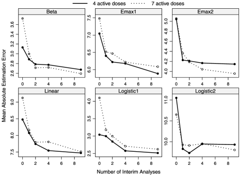
Figure 3: Mean absolute estimation error for MED estimation.

In Figure 3 we display, for each simulation scenario, the mean absolute estimation error for the MED against the number of interim analyses. In all scenarios one observes a benefit from adapting, while most of the improvement is already achieved after 1, 2 or 4 interim analyses. The largest relative improvement (comparing no adaptations vs 9 adaptations) can be observed for the Logistic₁ and the Beta model scenarios, particularly in the case of 7 active doses. The worst relative improvement can be observed for the Logistic₂ scenario, where the overall largest absolute estimation error can be observed. This is not surprising, because even when adapting one cannot achieve a good design for this model, as there are no doses available for administration in the interval $(20,50)$ containing the MED; see also Figure 1. It is remarkable to see that adaptation also works in the linear model scenario, although the linear model is not included in the candidate model set. It seems that other models in the candidate set are able to capture the shape of a linear model reasonably well.

The comparison between 4 and 7 active doses is not entirely clear. If no interim analyses are performed, it seems that the design with a balanced allocation across the 4 active doses is slightly better than the design with a balanced allocation across all 7 active doses. If one decides to adapt, however, it seems beneficial in some cases to have more doses available, particularly if many interim analyses are performed, while in other cases 4 active doses are sufficient.

To illustrate how adaptation changes the allocation of patients to the different doses, we display in Figure 4 the average patient allocations for the Emax₂ model after 1, 2, 4 and 9 interim analyses and with 7 available active doses. The adaptive design tends to allocate more patients both on placebo and nearby the actual MED. This is intuitively plausible, as the MED estimate depends on the precision of the estimated placebo effect as well as of the estimated function $f(\cdot)$ around the true MED. It also follows from Figure 4 that for a large number of interim analyses the overall allocation is close to the one under a locally optimal design for the Emax₂ model, with the variability in the allocations due to the uncertainty both in estimating the correct model and the model parameters at the interim analysis. Similar conclusions also hold for other models than the Emax₂ model (not reported here).

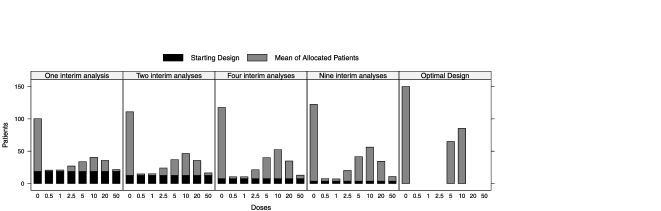
Figure 4: Average patient allocation after 1, 2, 4 and 9 interim analysis under the Emax₂ model. Last panel: locally MED-optimal design for the Emax₂ model with true MED${}={}$7.7.

We now investigate to which extent the precision gain observed in Figure 3 translates into sample size savings when performing an adaptive design. In other words, how many additional patients are required for a nonadaptive, balanced design to achieve a similar estimation error as with an adaptive design using 300 patients. We again considered the Emax₂ model and iterated the total sample size until the mean absolute estimation error was approximately 4 (which is the mean absolute estimation error obtained after 9 interim analyses, as seen in Figure 3). For both design options with 4 and 7 active doses, this was achieved after roughly 500 patients. Thus, using a nonadaptive, balanced design, one would need 200 additional patients to achieve a similar precision in MED estimation as compared to an adaptive design using 300 patients.

The adaptive design benefits observed so far depend on several input parameters, such as the starting design for the first stage. One may argue that starting with a bad design that allocates patients at the “wrong” doses may be improved by adapting at one or more interim looks. On the other hand, starting with a good design may lead to adaptations following random noise at the interim analyses. To illustrate this effect, we report the results for the simulations under the Logistic₁ model (similar results were also obtained for other models and scenarios, but are not reported here). We used four different starting designs. We used ${\mathbf{w}}=(0.35,0.03,0.22,0.35,0.05)$ and ${\mathbf{w}}=(0.35,0.02,0.02,0.02,0.02,0.20,0.30,0.07)$ as good starting designs with 4 and 7 active doses, respectively. These designs work well because they allocate patients on placebo and around the MED, while keeping some mass on the remaining doses. In addition, we used ${\mathbf{w}}=(0.1,0.3,0.05,0.05,0.5)$ and ${\mathbf{w}}=(0.1,0.2,0.22,0.02,0.02,0.02,0.02,0.4)^{\prime}$ as bad starting designs, as they have relatively few patients on placebo and around the MED. It follows from Figure 5 that substantial improvements are possible when using bad starting designs. On the other hand, for good starting designs no benefit is achieved by adapting and the performance may even deteriorate, because the possibility of adapting may lead one to deviate from the already good starting design. In practice, one does not know whether an employed design is good or bad, but one should keep in mind the possibility that adaptive designs will not always improve upon the initial design.

Figure 5: Mean absolute estimation error for MED estimation, under the the Logistic₁ model for good and bad starting designs.

To further investigate the robustness of the proposed methods, we repeated the simulation study from Figure 3 by increasing the standard deviation to 450 ml and 700 ml. The overall results remain similar, but with increased absolute estimation errors. However, the relative benefit of 9 interim analyses vs. no adaptation decreases slightly. Due to the larger noise, one obtains less reliable information at an interim analysis and one may end up with a worse design for the next stage. We also investigated the effect of prior misspecification. For this purpose we misspecified the prior means or prior modes by adding or subtracting 20% of the true value, but leaving the variability (variance of baseline and maximum effect and the value $S$ for the beta distribution) unchanged as in the original simulations. The results are largely identical to those presented in Figure 3, indicating that the proposed methods are robust under moderate prior misspecifications.

4.3 Conclusions for asthma study

Many more simulations than presented above were conducted at the planning stage of the asthma study to address the four questions stated in Section 2. Regarding question (A), it was felt that the potential benefits of conducting an adaptive design (more precise MED estimation) outweighed the additional logistical requirements, especially in view of the perceived sample size gain of 100–200 patients when compared to a fixed-sample study designed to achieve a similar precision. For question (B) it was decided to have one interim analysis: based on Figure 3 and other simulation results, the potential further reduction of the mean absolute estimation error with two or more interim analyses was perceived as too small to justify the additional logistical complexity.

For similar reasons, it was decided against having all seven actives doses from the beginning on question (C). Instead, 150 patients ought to be allocated equally across the four active doses 2.5, 10, 20, 50 (plus placebo) in the first stage. Once the interim results are available and analyzed with the methods from Section 3, however, patients could be allocated to all seven active doses (or a subset thereof) in the second stage. For practical reasons, the clinical team decided to incorporate constraints on the minimum number of patients allocated per dose in the second stage: if the algorithm would allocate less than 5% of the patients on a certain dose, that dose would be dropped altogether and the corresponding patients reallocated to the remaining doses.

5 Discussion

Motivated by a dose finding study in moderate persistent asthma, we described a response-adaptive approach that addresses common challenges encountered in dose-finding studies: multiple objectives, model uncertainty, and large variability. When planning an adaptive dose-finding design it is important to realize that it may not always be better than a nonadaptive design. It is necessary to employ a factored view, as many parameters may impact the performance of a study design. Often, an unbalanced fixed-sample design derived from optimal design theory might already provide benefit over a balanced fixed-sample design and adaptation may not bring further advantages, particularly if the variability is large (which is common in practice). Thus, adaptive designs are promising in situations where the initial design is not good and/or interim parameter estimates have low variability. In practice, one never knows how good the initial design will be, before trial start, and adaptive designs may guard against bad initial designs. However, the benefits of adaptive dose-finding designs have to be balanced against the increased logistical requirements to implement processes for repeated data collection, cleaning and analyses, to maintain trial integrity and validity, and to overcome potential challenges in drug manufacturing and supply.

In this paper we focused on designs based on the compound optimality criterion (4) to address model uncertainty and to minimize the variance of $\widehat{\mathrm{MED}}$. The criterion depends on the parameters of the different dose-response models as well as on the model probabilities and we used a Bayesian approach to continuously update parameter values and model probabilities based on the information accrued in the trial. The approach was implemented based on optimization and numerical quadrature, so that computationally intensive Markov chain Monte Carlo techniques could be avoided. Computational efficiency is of extreme importance, as the frequentist operating characteristics of any adaptive design methodology needs to be evaluated in extensive simulations under multiple scenarios.

The proposed method can be extended immediately if alternative optimality criteria [such as ED_p- or D-optimal designs, see Dette et al. (2010)] or mixtures thereof are of interest. Alternatively, optimal discrimination designs could be applied that allow one to differentiate among several candidate nonlinear regression models [Atkinson and Fedorov (1975), Dette and Titoff (2009)]. It would be interesting to address multiple objectives by considering different optimality criteria at different stages, such as using a model discrimination design in earlier stages, and MED-optimal design in later stages. This will be investigated in future research, but see Dragalin et al. (2010) for initial results.

The R functions used for the simulations are available with theDoseFinding R package [see Bornkamp, Pinheiro and Bretz (2010)].

Appendix: Proof of Theorem 3.1

Obviously the first part of the theorem follows from the lower bound (7) on the efficiency. For a proof of (7) let $\gamma=N_{\mathrm{old}}/(N_{\mathrm{old}}+N_{\mathrm{next}})\in(0,1)$ and note that the total information of the experiment in the $m$th model is given by

$$\hskip 20.0pt\mathbf{M}_{m}(\bolds\theta,\mathbf{w}_{\mathrm{old}},\mathbf{w}_{\mathrm{next}})=\gamma\mathbf{M}_{m}(\bolds\theta_{m},\mathbf{w}_{\mathrm{old}})+(1-\gamma)\mathbf{M}_{m}(\bolds\theta_{m},\mathbf{w}_{\mathrm{next}}),$$ (8)

where we collect in the vector $\bolds{\theta}=(\bolds\theta_{1},\ldots,\bolds\theta_{M})$ the parameters of the different models. Define a block diagonal matrix by

$$\overline{\mathbf{M}}(\bolds\theta_{m},\mathbf{w}_{\mathrm{old}},\mathbf{w}_{\mathrm{next}})$$

(9)

$$\qquad=\operatorname{diag}(\mathbf{M}_{1}(\bolds\theta_{m},\mathbf{w}_{\mathrm{old}},\mathbf{w}_{\mathrm{next}}),\ldots,\mathbf{M}_{M}(\bolds\theta_{M},\mathbf{w}_{\mathrm{old}},\mathbf{w}_{\mathrm{next}}))$$

(all other entries in this matrix are 0) and, similarly,

$$K=\operatorname{diag}(c_{1}(\bolds\theta_{1}),\ldots,c_{M}(\bolds\theta_{M})),$$

where the vector $c_{m}(\bolds\theta)$ is given by $c_{m}(\bolds\theta)=\bolds\nabla b_{m}(\bolds\theta),m=1,\ldots,M$. For a design $\mathbf{w}_{\mathrm{next}}$, such that $c_{m}(\bolds\theta)\in\operatorname{Range}(\mathbf{M}_{m}(\bolds\theta_{m},\mathbf{w}_{\mathrm{old}},\mathbf{w}_{\mathrm{next}}))$ $(m=1,\ldots,M)$, we consider the information matrix

$$C_{K}(\overline{\mathbf{M}}(\bolds\theta,\mathbf{w}_{\mathrm{old}},\mathbf{w}_{\mathrm{next}})) = (K^{T}\overline{\mathbf{M}}^{\,-}(\bolds\theta,\mathbf{w}_{\mathrm{old}},\mathbf{w}_{\mathrm{next}})K)^{-1}$$

$$= \operatorname{diag}((c^{T}_{1}(\bolds\theta_{1})\mathbf{M}^{-}_{1}(\bolds\theta_{1},\mathbf{w}_{\mathrm{old}},\mathbf{w}_{\mathrm{next}})c_{1}(\bolds\theta_{1}))^{-1},\ldots,$$

$$\hskip 28.0pt(c^{T}_{M}(\bolds\theta_{M})\mathbf{M}^{-}_{M}(\bolds\theta_{M},\mathbf{w}_{\mathrm{old}},\mathbf{w}_{\mathrm{next}})c_{M}(\bolds\theta_{M}))^{-1}).$$

Note that the optimal design maximizes

$$\Psi^{-1}(\mathbf{w}_{\mathrm{next}}) = \frac{N_{\mathrm{old}}+N_{\mathrm{next}}}{\sigma^{2}}\cdot\Phi_{\alpha}(C_{K}(\overline{\mathbf{M}}(\bolds\theta,\mathbf{w}_{\mathrm{old}},\mathbf{w}_{\mathrm{next}})))$$

$$= \frac{N_{\mathrm{old}}+N_{\mathrm{next}}}{\sigma^{2}}\prod^{M}_{m=1}(c^{T}_{m}(\bolds\theta)\mathbf{M}^{-}_{M}(\bolds\theta_{m},\mathbf{w}_{\mathrm{old}},\mathbf{w}_{\mathrm{next}})c_{m}(\bolds\theta))^{-\alpha_{m}},$$

where the last identity defines the criterion $\Phi_{\alpha}$ and we have used the notation $\Phi_{\alpha}(\operatorname{diag}(\lambda_{1},\ldots,\lambda_{M}))=\prod^{M}_{m=1}\lambda^{\alpha_{m}}_{m}$. Now according to Theorem 1 in Dette (1996), a lower bound for the efficiency of the design $\mathbf{w}_{\mathrm{next}}$

$$r(\mathbf{w})=\frac{\psi^{-1}(\mathbf{w})}{\psi^{-1}(\mathbf{w}_{\mathrm{opt}})}=\frac{\Phi_{\alpha}(C_{k}(\overline{\mathbf{M}}(\bolds\theta,\mathbf{w}_{\mathrm{old}},\mathbf{w}_{\mathrm{next}})))}{\max_{\mathbf{v}\in\mathbb{S}^{k}}\Phi_{\alpha}(C_{K}(\overline{\mathbf{M}}(\bolds\theta,\mathbf{w}_{\mathrm{old}},\mathbf{v})))}$$

is obtained as

$$e=\Bigl{[}\min_{\mathbf{G}}\max_{A\in\mathcal{A}}\operatorname{tr}\{\mathbf{G}KC_{K}(\overline{\mathbf{M}}(\bolds\theta,\mathbf{w}_{\mathrm{old}},\mathbf{w}_{\mathrm{next}}))$$

$$\hphantom{e=\Bigl{[}\min_{\mathbf{G}}\max_{A\in\mathcal{A}}\operatorname{tr}\{}{}\times\mathbf{E}C_{K}(\overline{\mathbf{M}}(\bolds\theta,\mathbf{w}_{\mathrm{old}},\mathbf{w}_{\mathrm{next}}))K^{T}\mathbf{G}^{T}A\}\Bigr{]}^{-1},$$

where the minimum is taken over the set of all generalized inverses of the matrix $\overline{\mathbf{M}}(\bolds\theta,\mathbf{w}_{\mathrm{old}},\mathbf{w}_{\mathrm{next}})$ and the set $\mathcal{A}$ is defined by

$$\mathcal{A}=\{\overline{\mathbf{M}}(\bolds\theta,\mathbf{w}_{\mathrm{old}},\mathbf{v})\mid\mathbf{v}\in\mathbb{S}^{k}\}$$

and the matrix $\mathbf{E}$ is given by

$$\mathbf{E}=\operatorname{diag}(\alpha_{1}c^{T}_{1}(\bolds\theta)\mathbf{M}^{-}_{1}(\bolds\theta_{1},\mathbf{w}_{\mathrm{old}},\mathbf{v})c_{1}(\bolds\theta),\ldots,\alpha_{M}c^{T}_{M}(\bolds\theta)\mathbf{M}^{-}_{M}(\bolds\theta_{M},\mathbf{w}_{\mathrm{old}},\mathbf{v})c_{m}).$$

Therefore, observing the identity

$$\mathbf{M}_{m}(\bolds\theta_{m},\mathbf{w}_{\mathrm{old}},\mathbf{v})=\mathbf{M}_{m}(\bolds\theta_{m},\mathbf{w}_{\mathrm{old}},\mathbf{w}_{\mathrm{next}})+(1-\gamma)\bigl{(}\mathbf{M}(\bolds\theta_{m},\mathbf{v})-\mathbf{M}(\bolds\theta,\mathbf{w}_{\mathrm{next}})\bigr{)},$$

we obtain

$$e = \Biggl{[}1+(1-\gamma)\min_{\mathbf{G}_{m}}\max_{v\in\mathbb{S}^{k}}\sum^{M}_{m=1}\alpha_{m}c^{T}_{m}(\bolds\theta_{m})\mathbf{G}^{T}_{m}\bigl{(}\mathbf{M}_{m}(\bolds\theta_{m},\mathbf{v})-\mathbf{M}_{m}(\bolds\theta_{m},\mathbf{w}_{\mathrm{next}})\bigr{)}$$

$$\hphantom{\biggl{[}1+(1-\gamma)\min_{\mathbf{G}_{m}}\max_{v\in\mathbb{S}^{k}}\sum^{M}_{m=1}}\hskip 45.0pt{}\times\mathbf{G}_{m}c_{m}(\bolds\theta)/(c^{T}_{m}(\bolds\theta_{m})\mathbf{G}_{m}c_{m}(\bolds\theta_{m}))\Biggr{]}^{-1}$$

$$\geq \Biggl{[}\min_{\mathbf{G}_{1},\ldots,\mathbf{G}_{m}}\max_{d\in\{d_{1},\ldots,d_{k}\}}\sum^{M}_{m=1}\alpha_{m}\frac{(g^{T}_{m}(d,\bolds\theta_{m})\mathbf{G}_{m}c_{m}(\bolds\theta_{m}))^{2}}{c^{T}_{m}(\bolds\theta_{m})\mathbf{G}_{m}c_{m}(\bolds\theta_{m})}$$

$$\hphantom{\biggl{[}\min_{\mathbf{G}_{1},\ldots,\mathbf{G}_{m}}\max_{d\in\{d_{1},\ldots,d_{k}\}}}{}\Big{/}\sum^{M}_{m=1}\alpha_{m}\frac{c^{T}_{m}(\bolds\theta_{m})\mathbf{G}^{T}_{m}M_{m}(\bolds\theta_{m},\mathbf{w}_{\mathrm{next}})\mathbf{G}_{m}c_{m}(\bolds\theta_{m})}{c^{T}_{m}(\bolds\theta_{m})\mathbf{G}_{m}c_{m}(\bolds\theta_{m})}\Biggr{]}^{-1},$$

where we have used the inequality

$$[1+(1-\gamma)(A-B)]^{-1}\geq\biggl{[}\frac{A}{B}\biggr{]}^{-1}$$

for $A\geq B\geq 0$, $(1-\gamma)B\leq 1$ and standard arguments in design theory.

References

- Atkinson, Donev and Tobias (2007) {bbook}[mr] \bauthor\bsnmAtkinson, \bfnmA. C.\binitsA. C., \bauthor\bsnmDonev, \bfnmA. N.\binitsA. N. and \bauthor\bsnmTobias, \bfnmR. D.\binitsR. D. (\byear2007). \btitleOptimum Experimental Designs, with SAS. \bseriesOxford Statistical Science Series \bvolume34. \bpublisherOxford Univ. Press, \baddressOxford. \bidmr=2323647 \endbibitem
- Atkinson and Fedorov (1975) {barticle}[mr] \bauthor\bsnmAtkinson, \bfnmA. C.\binitsA. C. and \bauthor\bsnmFedorov, \bfnmV. V.\binitsV. V. (\byear1975). \btitleOptimal design: Experiments for discriminating between several models. \bjournalBiometrika \bvolume62 \bpages289–303. \bidmr=0381163 \endbibitem
- Baltagi (2008) {bbook}[mr] \bauthor\bsnmBaltagi, \bfnmBadi H.\binitsB. H. (\byear2008). \btitleEconometrics, \bedition4th ed. \bpublisherSpringer, \baddressBerlin. \endbibitem
- Berger and Pericchi (1996) {barticle}[mr] \bauthor\bsnmBerger, \bfnmJames O.\binitsJ. O. and \bauthor\bsnmPericchi, \bfnmLuis R.\binitsL. R. (\byear1996). \btitleThe intrinsic Bayes factor for model selection and prediction. \bjournalJ. Amer. Statist. Assoc. \bvolume91 \bpages109–122. \bidmr=1394065 \endbibitem
- Biedermann, Dette and Pepelyshev (2006) {barticle}[mr] \bauthor\bsnmBiedermann, \bfnmStefanie\binitsS., \bauthor\bsnmDette, \bfnmHolger\binitsH. and \bauthor\bsnmPepelyshev, \bfnmAndrey\binitsA. (\byear2006). \btitleSome robust design strategies for percentile estimation in binary response models. \bjournalCanad. J. Statist. \bvolume34 \bpages603–622. \biddoi=10.1002/cjs.5550340404, mr=2347048 \endbibitem
- Bornkamp (2006) {bmisc}[auto:STB—2010-11-18—09:18:59] \bauthor\bsnmBornkamp, \bfnmB.\binitsB. (\byear2006). \bhowpublishedComparison of model-based and model-free approaches for the analysis of dose-response studies. Diploma thesis, Fakultät Statistik, Technische Univ. Dortmund. Available at http://www.statistik.uni-dortmund.de/~bornkamp/ diplom.pdf. \endbibitem
- Bornkamp, Pinheiro and Bretz (2010) {bmisc}[auto:STB—2010-11-18—09:18:59] \bauthor\bsnmBornkamp, \bfnmB.\binitsB., \bauthor\bsnmPinheiro, \bfnmJ.\binitsJ. and \bauthor\bsnmBretz, \bfnmF.\binitsF. (\byear2010). \bhowpublishedDoseFinding: Planning and analyzing dose finding experiments. R package version 0.4-1. \endbibitem
- Bretz, Pinheiro and Branson (2005) {barticle}[mr] \bauthor\bsnmBretz, \bfnmF.\binitsF., \bauthor\bsnmPinheiro, \bfnmJ. C.\binitsJ. C. and \bauthor\bsnmBranson, \bfnmM.\binitsM. (\byear2005). \btitleCombining multiple comparisons and modeling techniques in dose-response studies. \bjournalBiometrics \bvolume61 \bpages738–748. \biddoi=10.1111/j.1541-0420.2005.00344.x, mr=2196162 \endbibitem
- Bretz et al. (2008) {barticle}[mr] \bauthor\bsnmBretz, \bfnmFrank\binitsF., \bauthor\bsnmHsu, \bfnmJason\binitsJ., \bauthor\bsnmPinheiro, \bfnmJosé\binitsJ. and \bauthor\bsnmLiu, \bfnmYi\binitsY. (\byear2008). \btitleDose finding—a challenge in statistics. \bjournalBiom. J. \bvolume50 \bpages480–504. \biddoi=10.1002/bimj.200810438, mr=2526514 \endbibitem
- Chaloner and Verdinelli (1995) {barticle}[mr] \bauthor\bsnmChaloner, \bfnmKathryn\binitsK. and \bauthor\bsnmVerdinelli, \bfnmIsabella\binitsI. (\byear1995). \btitleBayesian experimental design: A review. \bjournalStatist. Sci. \bvolume10 \bpages273–304. \bidmr=1390519 \endbibitem
- Chatfield (1995) {barticle}[auto:STB—2010-11-18—09:18:59] \bauthor\bsnmChatfield, \bfnmC.\binitsC. (\byear1995). \btitleModel uncertainty, data mining and statistical inference. \bjournalJ. Roy. Statist. Soc. Ser. A \bvolume158 \bpages419–466. \endbibitem
- Cook and Wong (1994) {barticle}[mr] \bauthor\bsnmCook, \bfnmR. Dennis\binitsR. D. and \bauthor\bsnmWong, \bfnmWeng Kee\binitsW. K. (\byear1994). \btitleOn the equivalence of constrained and compound optimal designs. \bjournalJ. Amer. Statist. Assoc. \bvolume89 \bpages687–692. \bidmr=1294092 \endbibitem
- Dette (1996) {bincollection}[mr] \bauthor\bsnmDette, \bfnmHolger\binitsH. (\byear1996). \btitleLower bounds for efficiencies with applications. In \bbooktitleResearch Developments in Probability and Statistics \bpages111–124. \bpublisherVSP, \baddressUtrecht. \bidmr=1462412 \endbibitem
- Dette and Titoff (2009) {barticle}[mr] \bauthor\bsnmDette, \bfnmHolger\binitsH. and \bauthor\bsnmTitoff, \bfnmStefanie\binitsS. (\byear2009). \btitleOptimal discrimination designs. \bjournalAnn. Statist. \bvolume37 \bpages2056–2082. \biddoi=10.1214/08-AOS635, mr=2533479 \endbibitem
- Dette et al. (2008) {barticle}[mr] \bauthor\bsnmDette, \bfnmHolger\binitsH., \bauthor\bsnmBretz, \bfnmFrank\binitsF., \bauthor\bsnmPepelyshev, \bfnmAndrey\binitsA. and \bauthor\bsnmPinheiro, \bfnmJosé\binitsJ. (\byear2008). \btitleOptimal designs for dose-finding studies. \bjournalJ. Amer. Statist. Assoc. \bvolume103 \bpages1225–1237. \biddoi=10.1198/016214508000000427, mr=2462895 \endbibitem
- Dette et al. (2010) {barticle}[mr] \bauthor\bsnmDette, \bfnmH.\binitsH., \bauthor\bsnmKiss, \bfnmC.\binitsC., \bauthor\bsnmBevanda, \bfnmM.\binitsM. and \bauthor\bsnmBretz, \bfnmF.\binitsF. (\byear2010). \btitleOptimal designs for the emax, log-linear and exponential models. \bjournalBiometrika \bvolume97 \bpages513–518. \biddoi=10.1093/biomet/asq020, mr=2650755 \endbibitem
- Dragalin, Hsuan and Padmanabhan (2007) {barticle}[mr] \bauthor\bsnmDragalin, \bfnmVladimir\binitsV., \bauthor\bsnmHsuan, \bfnmFrancis\binitsF. and \bauthor\bsnmPadmanabhan, \bfnmS. Krishna\binitsS. K. (\byear2007). \btitleAdaptive designs for dose-finding studies based on sigmoid model. \bjournalJ. Biopharm. Statist. \bvolume17 \bpages1051–1070. \biddoi=10.1080/10543400701643954, mr=2414561 \endbibitem
- Dragalin et al. (2010) {bmisc}[auto:STB—2010-11-18—09:18:59] \bauthor\bsnmDragalin, \bfnmV.\binitsV., \bauthor\bsnmBornkamp, \bfnmB.\binitsB., \bauthor\bsnmBretz, \bfnmF.\binitsF., \bauthor\bsnmMiller, \bfnmF.\binitsF., \bauthor\bsnmPadmanabhan, \bfnmS. K.\binitsS. K., \bauthor\bsnmPatel, \bfnmN.\binitsN., \bauthor\bsnmPerevozskaya, \bfnmI.\binitsI., \bauthor\bsnmPinheiro, \bfnmJ.\binitsJ. and \bauthor\bsnmSmith, \bfnmJ. R.\binitsJ. R. (\byear2010). \bhowpublishedA simulation study to compare new adaptive dose-ranging designs. Statistics in Biopharmaceutical Research 2 487–512. \endbibitem
- Draper (1995) {barticle}[mr] \bauthor\bsnmDraper, \bfnmDavid\binitsD. (\byear1995). \btitleAssessment and propagation of model uncertainty. \bjournalJ. Roy. Statist. Soc. Ser. B \bvolume57 \bpages45–97. \bnoteWith discussion and a reply by the author. \bidmr=1325378 \endbibitem
- Fang and Wang (1994) {bbook}[mr] \bauthor\bsnmFang, \bfnmK. T.\binitsK. T. and \bauthor\bsnmWang, \bfnmY.\binitsY. (\byear1994). \btitleNumber-theoretic Methods in Statistics. \bseriesMonographs on Statistics and Applied Probability \bvolume51. \bpublisherChapman & Hall, \baddressLondon. \bidmr=1284470 \endbibitem
- Fedorov and Leonov (2001) {barticle}[auto:STB—2010-11-18—09:18:59] \bauthor\bsnmFedorov, \bfnmV.\binitsV. and \bauthor\bsnmLeonov, \bfnmS.\binitsS. (\byear2001). \btitleOptimal design of dose response experiments: A model-oriented approach. \bjournalDrug Information Journal \bvolume35 \bpages1373–1383. \endbibitem
- Golub and Pereyra (2003) {barticle}[mr] \bauthor\bsnmGolub, \bfnmGene\binitsG. and \bauthor\bsnmPereyra, \bfnmVictor\binitsV. (\byear2003). \btitleSeparable nonlinear least squares: The variable projection method and its applications. \bjournalInverse Problems \bvolume19 \bpagesR1–R26. \biddoi=10.1088/0266-5611/19/2/201, mr=1991786 \endbibitem
- Hjorth (1994) {bbook}[mr] \bauthor\bsnmHjorth, \bfnmJ. S. Urban\binitsJ. S. U. (\byear1994). \btitleComputer Intensive Statistical Methods: Validation, Model Selection, and Bootstrap. \bpublisherChapman & Hall, \baddressLondon. \bidmr=1270448 \endbibitem
- Kass and Raftery (1995) {barticle}[auto:STB—2010-11-18—09:18:59] \bauthor\bsnmKass, \bfnmR.\binitsR. and \bauthor\bsnmRaftery, \bfnmA.\binitsA. (\byear1995). \btitleBayes factors. \bjournalJ. Amer. Statist. Assoc. \bvolume90 \bpages773–795. \endbibitem
- King and Wong (2004) {barticle}[mr] \bauthor\bsnmKing, \bfnmJoy\binitsJ. and \bauthor\bsnmWong, \bfnmWeng Kee\binitsW. K. (\byear2004). \btitleOptimal designs for the power logistic model. \bjournalJ. Statist. Comput. Simul. \bvolume74 \bpages779–791. \biddoi=10.1080/0094965031000115402, mr=2083103 \endbibitem
- Läuter (1974) {barticle}[mr] \bauthor\bsnmLäuter, \bfnmElisabeth\binitsE. (\byear1974). \btitleExperimental design in a class of models. \bjournalMath. Operationsforsch. Statist. \bvolume5 \bpages379–398. \bidmr=0440812 \endbibitem
- Miller, Guilbaud and Dette (2007) {barticle}[mr] \bauthor\bsnmMiller, \bfnmFrank\binitsF., \bauthor\bsnmGuilbaud, \bfnmOlivier\binitsO. and \bauthor\bsnmDette, \bfnmHolger\binitsH. (\byear2007). \btitleOptimal designs for estimating the interesting part of a dose-effect curve. \bjournalJ. Biopharm. Statist. \bvolume17 \bpages1097–1115. \biddoi=10.1080/10543400701645140, mr=2414564 \endbibitem
- Müller et al. (2006) {barticle}[auto:STB—2010-11-18—09:18:59] \bauthor\bsnmMüller, \bfnmP.\binitsP., \bauthor\bsnmBerry, \bfnmD. A.\binitsD. A., \bauthor\bsnmGrieve, \bfnmA. P.\binitsA. P. and \bauthor\bsnmKrams, \bfnmM.\binitsM. (\byear2006). \btitleA Bayesian decision-theoretic dose-finding trial. \bjournalDecision Analysis \bvolume3 \bpages197–207. \endbibitem
- O’Hagan (1995) {barticle}[mr] \bauthor\bsnmO’Hagan, \bfnmAnthony\binitsA. (\byear1995). \btitleFractional Bayes factors for model comparison. \bjournalJ. Roy. Statist. Soc. Ser. B \bvolume57 \bpages99–138. \bnoteWith discussion and a reply by the author. \bidmr=1325379 \endbibitem
- O’Hagan and Forster (2004) {bbook}[auto:STB—2010-11-18—09:18:59] \bauthor\bsnmO’Hagan, \bfnmA.\binitsA. and \bauthor\bsnmForster, \bfnmJ.\binitsJ. (\byear2004). \btitleKendall’s Advanced Theory of Statistics, Volume 2B: Bayesian Inference, \bedition2nd ed. \bpublisherArnold, \baddressLondon. \endbibitem
- Pinheiro, Bornkamp and Bretz (2006) {barticle}[mr] \bauthor\bsnmPinheiro, \bfnmJosé\binitsJ., \bauthor\bsnmBornkamp, \bfnmBjörn\binitsB. and \bauthor\bsnmBretz, \bfnmFrank\binitsF. (\byear2006). \btitleDesign and analysis of dose-finding studies combining multiple comparisons and modeling procedures. \bjournalJ. Biopharm. Statist. \bvolume16 \bpages639–656. \biddoi=10.1080/10543400600860428, mr=2252312 \endbibitem
- Pukelsheim (1993) {bbook}[mr] \bauthor\bsnmPukelsheim, \bfnmFriedrich\binitsF. (\byear1993). \btitleOptimal Design of Experiments. \bpublisherWiley, \baddressNew York. \bidmr=1211416 \endbibitem
- Ruberg (1995) {barticle}[pbm] \bauthor\bsnmRuberg, \bfnmS. J.\binitsS. J. (\byear1995). \btitleDose response studies. I. Some design considerations. \bjournalJ. Biopharm. Statist. \bvolume5 \bpages1–14. \bidpmid=7613556 \endbibitem
- Seber and Wild (1989) {bbook}[mr] \bauthor\bsnmSeber, \bfnmG. A. F.\binitsG. A. F. and \bauthor\bsnmWild, \bfnmC. J.\binitsC. J. (\byear1989). \btitleNonlinear Regression. \bpublisherWiley, \baddressNew York. \biddoi=10.1002/0471725315, mr=0986070 \endbibitem
- van der Vaart (1998) {bbook}[mr] \bauthor\bparticlevan der \bsnmVaart, \bfnmA. W.\binitsA. W. (\byear1998). \btitleAsymptotic Statistics. \bseriesCambridge Series in Statistical and Probabilistic Mathematics \bvolume3. \bpublisherCambridge Univ. Press, \baddressCambridge. \bidmr=1652247 \endbibitem
- Wathen and Thall (2008) {barticle}[mr] \bauthor\bsnmWathen, \bfnmJ. Kyle\binitsJ. K. and \bauthor\bsnmThall, \bfnmPeter F.\binitsP. F. (\byear2008). \btitleBayesian adaptive model selection for optimizing group sequential clinical trials. \bjournalStatist. Med. \bvolume27 \bpages5586–5604. \biddoi=10.1002/sim.3381, mr=2573771 \endbibitem
- Wu (1988) {bincollection}[auto:STB—2010-11-18—09:18:59] \bauthor\bsnmWu, \bfnmC. F. J.\binitsC. F. J. (\byear1988). \btitleOptimal design for percentile estimation of a quantal response curve. In \bbooktitleOptimal Design and Analysis of Experiments \bpages213–222. \bpublisherElsevier, \baddressAmsterdam. \endbibitem
- Zhou et al. (2003) {barticle}[mr] \bauthor\bsnmZhou, \bfnmXiaojie\binitsX., \bauthor\bsnmJoseph, \bfnmLawrence\binitsL., \bauthor\bsnmWolfson, \bfnmDavid B.\binitsD. B. and \bauthor\bsnmBélisle, \bfnmPatrick\binitsP. (\byear2003). \btitleA Bayesian -optimal and model robust design criterion. \bjournalBiometrics \bvolume59 \bpages1082–1088. \biddoi=10.1111/j.0006-341X.2003.00124.x, mr=2025133 \endbibitem
- Zhu and Wong (2000) {barticle}[pbm] \bauthor\bsnmZhu, \bfnmW.\binitsW. and \bauthor\bsnmWong, \bfnmW. K.\binitsW. K. (\byear2000). \btitleMultiple-objective designs in a dose-response experiment. \bjournalJ. Biopharm. Statist. \bvolume10 \bpages1–14. \bidpmid=10709797 \endbibitem
- Zhu and Wong (2001) {barticle}[auto:STB—2010-11-18—09:18:59] \bauthor\bsnmZhu, \bfnmW.\binitsW. and \bauthor\bsnmWong, \bfnmW. K.\binitsW. K. (\byear2001). \btitleBayesian optimal designs for estimating a set of symmetric quantiles. \bjournalStat. Med. \bvolume20 \bpages123–137. \endbibitem