The earth matter effects in neutrino oscillation experiments from Tokai to Kamioka and Korea.

Abstract

We study the earth matter effects in the Tokai-to-Kamioka-and-Korea experiment (T2KK), which is a proposed extension of the T2K (Tokai-to-Kamioka) neutrino oscillation experiment between J-PARC at Tokai and Super-Kamiokande (SK) in Kamioka, where an additional detector is placed in Korea along the same neutrino beam line. By using recent geophysical measurements, we examine the earth matter effects on the oscillation probabilities at Kamioka and Korea. The average matter density along the Tokai-to-Kamioka baseline is found to be 2.6 ${\rm g/cm}^{3}$, and that for the Tokai-to-Korea baseline is 2.85, 2.98, and 3.05 ${\rm g/cm}^{3}$ for the baseline length of $L$- = 1000, 1100, and 1200 km, respectively. The uncertainty of the average density is about $6\%$, which is determined by the uncertainty in the correlation between the accurately measured sound velocity and the matter density. The effect of the matter density distribution along the baseline is studied by using the step function approximation and the Fourier analysis. We find that the $\nu_{\mu}\to\nu_{e}$ oscillation probability is dictated mainly by the average matter density, with small but non-negligible contribution from the real part of the first Fourier mode. We also find that the sensitivity of the T2KK experiment on the neutrino mass hierarchy does not improve significantly by reducing the matter density error from $6\%$ to $3\%$, since the measurement is limited by statistics for the minimum scenario of T2KK with SK at Kamioka and a 100 kt detector in Korea considered in this report. The sensitivity of the T2KK experiment on the neutrino mass hierarchy improves significantly by splitting the total beam time into neutrino and anti-neutrino runs, because the matter effect term contributes to the oscillation amplitudes with the opposite sign.

KEK-TH-1100

1 Introduction

Many neutrino oscillation experiments have been performed to measure the neutrino oscillation parameters. In the three neutrino model, there are nine fundamental parameters; three masses ($m_{1}$, $m_{2}$, $m_{3}$), three mixing angles ($\theta_{12}$, $\theta_{13}$, $\theta_{23}$) and three phases ($\delta$, $\phi_{1}$, $\phi_{2}$) of the lepton-flavor-mixing matrix, MNS matrix [1]. Among the three CP phases, one ($\delta$) is lepton number conserving and two ($\phi_{1}$, $\phi_{2}$) are lepton number non-conserving phases of the neutrino Majorana masses. Out of the nine parameters, the neutrino-flavor oscillation experiments can measure six parameters; two mass-squared differences ($m^{2}_{2}-m^{2}_{1}$, $m^{2}_{3}-m^{2}_{1}$), all the three mixing angles ($\theta_{12}$, $\theta_{13}$, $\theta_{23}$), and the lepton number conserving phase ($\delta$). Among them, the magnitude of the larger mass-squared difference, $|m^{2}_{3}-m^{2}_{1}|$, and a mixing angle, $\theta_{23}$ , have been measured by the atmospheric neutrino experiments[2, 3], which have been confirmed by the accelerator based long-baseline (LBL) neutrino oscillation experiments, K2K [4] and MINOS [5]. The smaller mass-squared difference, $m^{2}_{2}-m^{2}_{1}$, and the corresponding mixing angle, $\theta_{12}$, have been measured by the solar neutrino oscillation experiments [6], and the KamLAND experiment [7] that observes the oscillation of reactor anti-neutrinos at more than 100 km distance. The third mixing angle, $\theta_{13}$, has been looked for in the oscillation of reactor anti-neutrinos at about 1km distance. No oscillation has been observed and only the upper bound on $\sin^{2}2\theta_{13}$ of about 0.14 has been reported [8, 9].

Summing up, out of the nine parameters of the three neutrino model, six parameters can be observed in neutrino-flavor oscillation experiments, among which $|m_{3}^{2}-m_{1}^{2}|$, $\theta_{23}$, $m_{2}^{2}-m_{1}^{2}$, and $\theta_{12}$ have been measured, and the upper bound on $\sin^{2}2\theta_{13}$ has been obtained. The goal of the next generation neutrino oscillation experiments is hence to determine the remaining parameters, ${\it i.e.}$, the sign of $m^{2}_{3}-m^{2}_{1}$ (the neutrino mass hierarchy pattern), a finite value of the third mixing angle $\theta_{13}$, and the CP violating phase of the lepton sector, $\delta$.

Several neutrino oscillation experiments are starting or being prepared aiming at the measurements of $\theta_{13}$, which can be categorized into two types; one is the next generation of reactor neutrino experiments, and the others are accelerator based neutrino oscillation experiments. Three experiments, Double CHOOZ [10], RENO [11], and Daya Bay[12], will be able to observe the oscillation (disappearance) of $\bar{\nu}_{e}$’s from reactors at about 1km distances if $\sin^{2}2\theta_{13}\lower 2.15277pt\hbox{$\;\buildrel>\over{\sim}\;$}0.01$. In accelerator based LBL experiments, $\nu_{\mu}$ or $\bar{\nu}_{\mu}$ beam from high energy $\pi^{+}$ or $\pi^{-}$ decay-in-flight, respectively, will be detected at a distance of a few to several hundred km’s away and the $\nu_{\mu}\to\nu_{e}$ or $\bar{\nu}_{\mu}\to\bar{\nu}_{e}$ transition is looked for. The transition rate is proportional to $\sin^{2}\theta_{13}$, and the next generation LBL experiments, the Tokai-to-Kamioka (T2K) experiment [13] and the NO$\nu$A experiment [14], have a chance to discover the $\nu_{\mu}\to\nu_{e}$   transition, if $\sin^{2}2\theta_{13}$ $\;\buildrel>\over{\sim}\;$0.02.

In this report, we focus our attention on the proposed one-beam two-detector experiment, the Tokai-to-Kamioka-and-Korea (T2KK) experiment [15, 16, 17, 18, 19, 20]. T2KK is an extension of the T2K experiment where an additional huge detector is placed in Korea along the T2K neutrino beam line between J-PARC at Tokai and Super-Kamiokande (SK) at Kamioka. We show the cross section view of the T2KK experiment in Fig. 1.

Figure 1: Schematic cross section view of the T2KK experiment when the center of the neutrino beam from J-PARC is $3^{\circ}~{}$ below the Super Kamiokande detector. The center of the beam is shown by the red arrows, and the black arrows show the baselines of a few off-axis beams (OAB).

The center of the T2K neutrino beam has been designed to go through the underground beneath SK so that an off-axis beam (OAB) between  $2^{\circ}~{}$ and $3^{\circ}~{}$ upward from the beam center can be observed at SK, in order to maximize the sensitivity to the $\nu_{\mu}\to\nu_{e}$ oscillation. It then follows that the center of the T2K beam reaches the sea level in the Japan/East sea, and the lower-side of the same beam at $0.5^{\circ}~{}$ or larger off-axis angle goes through Korea [15, 17]. Therefore, if we place an additional neutrino detector in Korea along the T2K beam line, we can perform two LBL experiments at the same time. It has been demonstrated that the T2KK experiment has an outstanding physics potential to determine the neutrino mass hierarchy pattern, normal ($m^{2}_{3}-m^{2}_{1}>0$) or inverted ($m^{2}_{3}-m^{2}_{1}<0$), and to determine the CP violating phase $\delta$ [16, 17, 18].

The key of determining the neutrino mass hierarchy pattern in the T2KK experiment is the earth matter effect, which arises from the coherent interaction of $\nu_{e}$ (or $\bar{\nu}_{e}$) off the electrons in the earth matter [21]. The matter effect enhances or suppresses the $\nu_{\mu}\to\nu_{e}$   oscillation probability, respectively, if the mass hierarchy pattern is normal ($m^{2}_{3}-m^{2}_{1}>0$) or inverted ($m^{2}_{3}-m^{2}_{1}<0$). Furthermore, the matter effect around the first oscillation maximum in Korea ($L\lower 2.15277pt\hbox{$\;\buildrel>\over{\sim}\;$}1000$ km) is significantly larger than the one at SK ($L=295$ km) because its magnitude grows with neutrino energy, and the oscillation phase is roughly proportional to the ratio $L/E$. Fortunately, we can observe the first oscillation maximum at both detectors efficiently, if a detector is placed in the east coast of Korea such that $0.5^{\circ}\sim 1^{\circ}$ OAB can be observed at $L\sim 1000$ km when the beam is adjusted to give the $3.0^{\circ}\sim 2.5^{\circ}$ OAB at SK [17, 18]. In a previous work [18], it has been found that the neutrino mass hierarchy can be determined most effectively by observing $0.5^{\circ}$ off-axis beam in Korea at $L\sim 1000$ km and $3.0^{\circ}$ off-axis beam at Kamioka. With this combination, the neutrino mass hierarchy pattern can be determined at 3-$\sigma$ level when $\sin^{2}2\theta_{13}\lower 2.15277pt\hbox{$\;\buildrel>\over{\sim}\;$}0.06$, if we place a 100 kt level Water $\check{\rm C}$erenkov detector in Korea during the T2K experimental period with $5\times 10^{21}$ POT (protons on target). This is the minimum scenario where no additional detector is placed in Kamioka and no increase is the J-PARC beam power is assumed. A 100 kt level fiducial volume for the detector in Korea is necessary in order to balance the statistics of SK with 20 kt at 1/3 the distance from the J-PARC. A more grandiose scenario with huge detector both at Kamioka and Korea has been considered in Ref. [16].

Since the earth matter effect is very important in estimating the physics discovery potential of the T2KK proposal, we study in this report its impacts and uncertainty in detail by using the recent geophysical measurements of the earth matter density beneath Japan, Japan/East sea, and Korea. Both the average and the distribution of the matter density along the Tokai-to-Kamioka and the Tokai-to-Korea baselines are studied, as well as their errors. We also examine the impact of using both of the neutrino and anti-neutrino beams, since the earth matter effect on the $\nu_{\mu}\to\nu_{e}$ and $\bar{\nu}_{\mu}\to\bar{\nu}_{e}$ transitions have opposite signs.

This paper is organized as follows. In section 2, we study the earth matter density profile along the Tokai-to-Kamioka and Tokai-to-Korea baselines, and then we evaluate the average and the Fourier modes of the matter densities along the baselines. In section 3, we discuss how to treat neutrino oscillations with non-uniform matter distributions. We obtain both the exact solution to the oscillation amplitudes and on approximate analytic expression for the oscillation probability that makes use of the Fourier series of the matter distribution along the baseline. In section 4, we introduce our analysis method that quantifies the sensitivity of the T2KK experiment on the neutrino mass hierarchy pattern by introducing a $\chi^{2}$ function that accounts for both statistical and systematic errors. In section 5, we discuss the matter effect dependence of the capability of determining the mass hierarchy pattern in the T2KK experiment. In section 6, we consider the matter effect for the anti-neutrino experiment, and examine the impact of combining both neutrino and anti-neutrino oscillation experiments. Finally, we summaries our findings in section 7. In Appendix, we give the second-order perturbation formula for the neutrino oscillation amplitudes in terms of the matter effect term and the smaller mass squared difference.

2 Earth matter profile along the T2KK baselines

In this section, we study the matter density distribution along the baselines of Tokai-to-Kamioka and Tokai-to-Korea, and then estimate the average and the Fourier modes of the matter profile along the baselines.

2.1 Tokai-to-Kamioka baseline

First, we show the Tokai-to-Kamioka (T2K) baseline and its cross section view along the baseline in Fig. 2.

Figure 2: Upper: The Tokai-to-Kamioka (T2K) baseline. The distance from J-PARC along the baseline is shown by tick marks every 50 km. The shaded region is called Fossa Magna [22], where the North American plate and the Eurasian plate meet. Lower: The cross section view of the T2K experiment. The horizontal line shows the distance from the J-PARC [25] and the vertical axis measures the depth from the sea level. The number in each region shows the mean matter density in units of ${\rm g/cm}^{3}$. The neutrino beam line between J-PARC and Kamioka is shown by an arc.

In the upper figure, the scale along the baseline shows the distance from J-PARC by tick marks every 50 km. The shaded region is called Fossa Magna [22], which is the border between the two continental plates, North American Plate and Eurasian Plate. In this region, the sediment layer is estimated as 6 times deeper than that in the surrounding region. The lower plot shows the cross section view of the T2K experiment. The horizontal line shows the distance from the J-PARC and the vertical axis gives the depth from the sea level. The number in each region stands for the average matter density in units of ${\rm g/cm}^{3}$. In this figure, the thickness of the sediment layer except for the Fossa Magna region is assumed to be $1\rm km$ [23] and we refer to the geological map in Ref. [24]. In Fossa Magna, the sediment layer is as deep as $6$ km [22], which is mainly composed of limestone and sandstone with others [24]. According to Ref. [22], the density of such sediment layer is $2.5{\rm g/cm}^{3}$. On the other hand, the sediment layer near Kamioka, $L>230$ km along the baseline, is mainly composed of granite whose density is about $2.8{\rm g/cm}^{3}$.

When we average out the matter density along the baseline shown in Fig. 2, we obtain the average density of 2.6 ${\rm g/cm}^{3}$, which is significantly lower than the value 2.8${\rm g/cm}^{3}$ quoted in the Letter of Intent (LOI) of the T2K experiment [13]. The difference is mainly due to Fossa Magna, whose lower density has not been taken into account in the past.

The error of the average density can be estimated from the error of the mean density in each region, and the uncertainty of the boundary of each layer. In most of research works in geophysics, these two values are evaluated by using the seismic wave observation. The mean value of the matter density is estimated from the velocity of the seismic wave in each region. In this work, we adopt the density-velocity correlation of Ref. [26] to estimate the matter density from the $p$-wave velocity.

Figure 3: The relation between the matter density and the $p$-wave sound velocity ($V_{p}$) according to Ref. [26]. The solid line gives the mean value of the density, and the dotted lines in both sides show the error of the estimated density. The dashed lines show how we estimate the density and its error when $V_{p}=6.5$ km/sec. The three square points are the reference points in Preliminarily Reference Earth Model (PREM) [27].

In Fig. 3, we show the density velocity relation. The solid line shows the relation between the sound velocity and the mean matter density according to Ref. [26], which can be expressed as

$$\rho=-0.00283V_{p}^{4}+0.0704V_{p}^{3}-0.598V_{p}^{2}+2.23V_{p}-0.7\,,$$ (1)

where $V_{p}$ is the $p$-wave sound velocity inside the matter in units of km/sec, and the matter density $\rho$ is in units of ${\rm g/cm}^{3}$. The dotted lines in both sides show the error of the estimated density, which is about $6\%$. The dashed lines show how we estimate the density and its error when $V_{p}=6.5$ km/sec. The three squares are the reference points shown in Preliminarily Reference Earth Model (PREM) [27], which is often used to estimate the average density along the baseline for various LBL experiments. These points lie close enough to the mean density line of eq. (1), confirming the consistency between the PREM and the other geological measurements. On the other hand, the location of the boundary is evaluated from the reflection point of the seismic wave. The error of the boundary depth between the sediment layer and the upper crust is estimated as $\pm 300$ m. It affects the average density along the T2K baseline only by 0.05$\%$, and it can be safely neglected. The error of the assumed sound velocity measurement at various location can also be neglected. In this report, we assume that the matter density error is determined by the $6\%$ systematic uncertainty in the density-velocity relation, which is taken to be common ($100\%$ correlation) at all location along the baseline. On the other hand, the error of the average matter density along the T2K baseline and the Tokai-to-Korea baselines are taken to be independent in order to make the most conservative estimate. The $6\%$ error adapted in this report is a factor of two larger than the error adapted in Refs. [17, 18]. The matter density error is expected to become smaller by making use of the information from the other measurements, e.g. the gravity anomaly, the magnetic anomaly, and by actually digging into the crust.

Figure 4: Fourier modes of the matter density distribution along the Tokai-to-Kamioka baseline in units of ${\rm g/cm}^{3}$. Black circles and white squares show the real and the imaginary parts of the Fourier coefficients, respectively.

We note that the density fluctuation along the T2K baseline of Fig. 2 from the average of 2.6 ${\rm g/cm}^{3}$ is about $8\%$, which is comparable to the $6\%$ error of the average matter density. It is therefore of our concern that the approximation of using only the average matter density along the baseline may not be accurate enough. In Ref. [23], the authors have shown that the Fourier analysis is useful to study the impacts of the matter density distribution. We therefore show the Fourier coefficients of the matter density profile along the Tokai-to-Kamioka baseline in Fig. 4. Black circles and white squares show the real and the imaginary parts of the Fourier modes in units of ${\rm g/cm}^{3}$, respectively, which are defined as

$$\rho(x) = \sum_{k=-\infty}^{\infty}\bar{\rho}_{k}{\rm exp}\left(-i\frac{2\pi kx}{L}\right)$$ (2)

$$= \bar{\rho}_{0}+2\sum^{\infty}_{k=1}\left[{\rm Re}\left(\bar{\rho}_{k}\right)\cos\left(\frac{2\pi kx}{L}\right)+{\rm Im}\left(\bar{\rho}_{k}\right)\sin\left(\frac{2\pi kx}{L}\right)\right]\,,$$

where $\rho(x)$ is the matter density along the baseline at a distance $x$ from J-PARC. Positive value of Re($\bar{\rho}_{1}$) is clearly due to the low density of Fossa Magna in the middle of the baseline, whereas the negative values of Im($\bar{\rho}_{2}$) and Im($\bar{\rho}_{3}$) reflect the high matter density in the Kamioka area that makes the distribution asymmetric about the half point $(x=L/2)$ of the baseline. We note, however, that the magnitude of all the Fourier modes is less than 0.05 ${\rm g/cm}^{3}$, which is less than $2\%$ of the average matter density of $\bar{\rho}_{0}=2.6{\rm g/cm}^{3}$. We can therefore expect that the fluctuation effect can be safely neglected in the T2K experiment, as will be verified below.

2.2 Tokai-to-Korea baselines

Let us now examine the matter density distribution along the Tokai-to-Korea baseline.

Figure 5: The surface map (up) of the Tokai-to-Kamioka-and-Korea (T2KK) experiment, the cross section view (middle) and the density distribution along the baselines (bottom). The center of the neutrino beam line is shown in the upper figure, along which the distance from J-PARC is given by the tick marks every 100 km. The three circles show the regions which have been studied by geophysicists; Yamato basin, Oki trough [28] and Tsushima/Ulleung basin [29, 30]. In the middle figure, the five curves show the baselines for $L=1000$, 1050, 1100, 1150 and 1200 km, where the horizontal axis gives the distance from J-PARC along the arc of the earth surface, and the vertical scale measures the location of the baseline below the sea level. The numbers in white squares represent the average matter density of the surrounding stratum, in units of ${\rm g}/{\rm cm}^{3}$.

In Fig. 5, we show the surface map of the T2KK experiment (up), its cross section view (middle), and the matter density distribution along the baselines (bottom). Along the center of the neutrino beam line shown in the surface map, the distance from J-PARC is given by tick marks every 100 km. The areas enclosed by the three circles show the regions which have been studied by geophysicists; Yamato basin, Oki trough [28] and Tsushima/Ulleung basin [29, 30]. In the middle figure, the five curves correspond to the baselines for $L=1000$, 1050, 1100, 1150 and 1200 km, where the horizontal axis measures the distance along the earth arc from J-PARC, and the vertical axis measures the location of the baselines below the sea level. The numbers in white squares represent the average matter density, in units of ${\rm g}/{\rm cm}^{3}$, of the surrounding stratum: the sediment layer (2.5), the upper crust (2.8), the lower crust (2.9), and the upper mantle (3.3). A lump of 3.1 ${\rm g/cm}^{3}$ at Korean coast is a lava boulder [30]. In order to produce this figure, we refer to the recent study on the Conrad discontinuity, the boundary between the upper and the lower crust, and on the Mohorovi$\check{\rm c}$i$\acute{\rm c}$ discontinuity (Moho-discontinuity), the boundary between the crust and the mantle, below Japan and Korea [31, 32]. Regarding the matter profile beneath the Japan/East sea, we divide the sea into three regions, Oki trough (east side) [28], Oki island (middle) [29], and Tsushima/Ulleung basin (west side)[30]. According to Refs. [28, 30], typical depths of the Conrad and the Moho-discontinuities below Oki trough (Tsushima/Ulleung basin) are 8 km (7km) and 20 km (17 km), respectively. On the other hand, Ref. [29] shows that they are 6km and 25 km, respectively, below the sea level at around Oki island. Although there is no direct measurement of the discontinuities along the Tokai-to-Korea baselines, we may assume that the depth of the discontinuities is roughly characterized by the depth of the seabed of each region. If the sea is shallower, the discontinuities should be deeper, and vice versa. Because the seabed above the baseline is rather flat the east and west sides of Oki islands, we obtain the estimates of Fig. 5 from the measured depths of the discontinuities in each region.

In addition, we adopt the following simple interpolations around the sea bounds. As for the Moho-discontinuity, we assume that it is connected from 32 km below the sea level at the Japanese coast, the point (380 km, 32 km) in the middle figure, to 20 km below the Japan/East sea at (440 km, 20 km) by a straight line as illustrated in the figure. It is at this point, about 60 km west from the coast along the beam direction, the depth of the Japan/East sea reaches 1 km, the average depth of Oki trough. As for the Oki island region, the Moho-discontinuity is connected by straight line from (600 km, 20 km) to (630 km, 25 km), flat from 630 km to 700 km, and then by another straight line from (700km, 25km) to (730km, 17 km). Near the Korean coast, it is connected by a straight line from (970km, 17km) to (990km, 32 km). Here the slope is shaper because the Korean coast is only about 20 km away from the western edge of Tsushima/Ulleung basin [30]. As for the Conrad discontinuity, we also assume the linear interpolation between (380 km, 15 km) and (440 km, 8 km) at the Japanese coast, (600km, 8km) and (630km, 5km) at east side of Oki island region, (700km, 5km) and (750km, 7km) at west side of Oki island region, and between (970 km, 7 km) and (990 km, 17 km) at the Korean coast. The lava bounder lies on top of the oblique section of the Moho-discontinuity and it is assumed to have the triangle shape along the cross section with the apexes at, (970 km, 17 km), (990km, 15km), and (990km, 30km) as also illustrated in the middle figure. Although the above treatments of the boundary conditions are very rough, we do not elaborate them further because the neutrino oscillation probabilities are very insensitive to the exact location of the boundaries.

With the above setting, we obtain the matter density distribution along the baselines shown in the bottom figure of Fig. 5. Here the horizontal axis measures the distance $x$ from J-PARC along the baseline. We assume that a detector in Korea is placed at the sea level (zero altitude) along the plane of the center and the center of the earth, at the distance $L$ from J-PARC. Along the baseline of length $L$, the point $x$ (km) away from J-PARC appears on the cross section figure in the middle of Fig. 5 at the distance $l$ (km) along the earth arc, and the depth $d$ (km) below the sea level;

$$l = R\arcsin\left(\frac{x}{R}\sqrt{\displaystyle\frac{R^{2}-L^{2}/4}{R^{2}-xL+x^{2}}}\right)$$ (3a)

$$= x\left\{1-\frac{x^{2}}{3R^{2}}+\frac{xL}{2R^{2}}-\frac{L^{2}}{8R^{2}}+{\it O}\left(R^{-4}\right)\right\},$$

$$d = R-\sqrt{x^{2}-xL+R^{2}}=\frac{x\left(L-x\right)}{2R}\left[1+{\it O}\left(R^{-3}\right)\right]\,,$$ (3b)

where $R$ is the radius of the earth, 6378.1 km. The five arcs are the cross section view of Fig. 5 are then obtained parametrically as ($l(x),d(x)$). It is also noted that $l$ is not much different from $x$ for $L\sim 1000$ km; $l$ is about $0.01\%$ shorter than $x$ at $\sim 300$ km, and $0.1\%$ longer $x$ at $x\sim 1000$ km. The effect of the lava boulder near the Korean coast is seen in the matter density distribution for $L=$ 1100 km and 1150 km. We also notice that the baseline for $L=1000$ km goes through the sediment layer (2.5 ${\rm g/cm}^{3}$) near the Korean east at $970{\rm km}\lower 2.15277pt\hbox{$\;\buildrel<\over{\sim}\;$}l\lower 2.15277pt\hbox{$\;\buildrel<\over{\sim}\;$}990$km ($969{\rm km}\lower 2.15277pt\hbox{$\;\buildrel<\over{\sim}\;$}x\lower 2.15277pt\hbox{$\;\buildrel<\over{\sim}\;$}989{\rm km}$). All the baselines go through the sediment layer near the J-PARC until the baseline reaches the depth of $d=$ 1 km ($0\lower 2.15277pt\hbox{$\;\buildrel<\over{\sim}\;$}x\lower 2.15277pt\hbox{$\;\buildrel<\over{\sim}\;$}10\sim 13$ km).

Let us now estimate the average matter density and its error along each baseline. Since the traveling distance in the mantle and that in the crust depend on the locations of their boundaries, the error of the average matter density is affected by the errors of the depths of the discontinuities. It is especially important for the Moho-discontinuity because the density difference between the lower crust and the upper mantle is as large as $0.4{\rm g/cm}^{3}$, which is about $13\%$ of their average. Therefore, we examine the impacts of varying the depth of the Moho-discontinuity on the average matter density.

Baseline length	The depth of the Moho-discontinuity below the sea level
$L$	$-3\sigma$	$-1\sigma$	mean	$+1\sigma$	$+3\sigma$
1000 km	2.923	2.900	2.854	2.854	2.854
1050 km	2.973	2.954	2.944	2.933	2.862
1100 km	3.001	2.988	2.980	2.971	2.952
1150 km	3.049	3.039	3.027	3.002	2.986
1200 km	3.054	3.052	3.051	3.049	3.036
Re$\bar{\rho}_{1}$ $(L=1000$ km)	$-0.097$	$-0.076$	$-0.031$	$-0.031$	$-0.031$
Re$\bar{\rho}_{1}$ $(L=1050$ km)	$-0.102$	$-0.098$	$-0.094$	$-0.090$	$-0.028$
Re$\bar{\rho}_{1}$ $(L=1100$ km)	$-0.117$	$-0.110$	$-0.101$	$-0.105$	$-0.099$

Table 1: Average matter density along the baselines of $L=1000$, 1050, 1100, 1150 and 1200 km, in units of ${\rm g/cm}^{3}$, for five possible locations of the Moho-discontinuity, which is the boundary between the lower crust and the upper mantle. The bottom three rows give the real part of the first Fourier coefficient of the matter density distribution along the $L=1000,1050,$ and 1100 km baselines.

In Table 1, we show the average matter density along the baselines of $L=1000$, 1050, 1100, 1150 and 1200 km, in units of ${\rm g/cm}^{3}$, for five locations of the Moho-discontinuity. The mean corresponds the depth of 20 km at $L\sim 500$ km and 17 km at $L\sim 800$ km in Fig. 5, $\pm 1\sigma~{}(\pm 3\sigma)$ corresponds to the overall shifts by $\pm 0.7$ km ($\pm 2$ km) of the Moho-discontinuity depth below the sea level.

Because longer baselines go through the upper mantle for a longer distance, the average density grows with $L$; 2.854 ${\rm g/cm}^{3}$ at $L=1000$ km to 2.944, 2.980, 3.027, and 3.051 ${\rm g/cm}^{3}$ at $L(\rm km)=$ 1050, 1100, 1150, and 1200, respectively. The average density at $L=1000$ km is quite sensitive to the rise of the Moho-discontinuity because the baseline almost touches the mantle at $L\sim 500$ km for the mean estimate, as shown in Fig. 5. The average density grows from $2.854{\rm g/cm}^{3}$ for the mean depth to $2.900{\rm g/cm}^{3}$, by $1.6\%$, if the Moho-discontinuity is only 0.7 km ($1\sigma$) higher than the present estimate. Although this is striking, the effect is significantly smaller than the $6\%$ overall uncertainty in the conversion of the sound velocity to the matter density. We therefore neglect the effect in the present study, but further geophysical studies may be desired if $L\sim 1000$ km baseline is chosen for the far detector location.

We also examine the impacts of the non-uniformity of the matter density distribution along the Tokai-to-Korea baseline.

Figure 6: Fourier coefficients of the density distribution along the Tokai-to-Korea baselines ; $L=1000$ km (a), and 1200 km (b). Black circles and white squares show the real and imaginary parts of the Fourier coefficients, respectively, and the cross symbols show the real parts estimated from PREM [27].

In Fig. 6, the black circles and white squares show, respectively, the real and imaginary parts of the Fourier coefficients of the matter density distribution along the baselines of $L=1000$ km (a) and 1200km (b). As a reference, we show by the cross symbols the real part of the Fourier coefficients of the matter density distribution of PREM [27]. The PREM generally gives symmetric matter distribution about $x=L/2$, and hence does not give imaginary cofficients. When we compare them with the distribution for the Tokia-to-Kamioka baseline of Fig. 4, we find that Re$(\bar{\rho}_{1})$ is now negative and its magnitude grows from 0.03 ${\rm g/cm}^{3}$ at $L=1000$ km to 0.14 ${\rm g/cm}^{3}$ at $L=1200$ km. We note here that Re($\bar{\rho}_{1}$) at $L=1000$ km depends strongly on the depth of the Moho-discontinuity, because whether the baseline goes through mantle or not affects the convexity of the matter density distribution significantly; see Fig. 5 and discussions on the average matter density above. In order to show this sensitivity, we give Re$(\bar{\rho}_{1}$) values for $L=1000$, 1050, and 1100 km in the bottom three rows of Table 1. It changes from $-0.03{\rm g/cm}^{3}$ to $-0.08{\rm g/cm}^{3}$ at $L=1000$ km by more than a factor of two, if the Moho-discontinuity is only $0.7$ km ($1\sigma$) shallower than our estimate of 20 km based on the measurement in Oki trough [28]. As for the $L=1050$ km, the Re($\bar{\rho}_{1}$) is almost insensitive to the depth of the Moho-discontinuity. Since the baseline of $L=1100$ km is more than 22 km below at Oki trough, the magnitude of Re($\bar{\rho}_{1}$) of $L=1100$ km is insensitive to the exact depth of the Moho-discontinuity.

Along the Tokai-to-Korea baseline, the convexity measure of $-{\rm Re}(\bar{\rho}_{1})/\bar{\rho}_{0}$ grows from $\sim 1\%$ ($\sim 3\%$ if the Moho-discontinuity is $3\%$ shallower than our estimate) at $L=1000$ km to $5\%$ at $L=1200$ km. Their effects are hence non-negligible even with the $6\%$ overall uncertainty in the average matter density. We also note that the negative sign of Im$(\bar{\rho}_{1})$ reflects the fact that the mantle is slightly closer to a far detector in Korea than J-PARC in Tokai.

2.3 Comparison with PREM

Before closing this section, we compare the matter density distribution of this work and those of the PREM [27], where the earth is a spherically symmetric ball such that the depth of the boundaries between adjacent layers are the same everywhere.

Figure 7: The cross section view of the T2KK experiment along the baselines according to Preliminarily Reference Earth Model (PREM) [27].

In Fig. 7, we show the cross section view of the T2KK experiment along the baselines according to PREM. Although the original PREM assumes that the sea covers whole of the earth down to 3 km from the sea level, we assume in this figure that none of the baselines go through the sea.

There are several notable differences between the matter density distribution of this work shown in Fig. 5 and that of PREM in Fig. 7. As for the T2K baseline, the Fossa Magna lies in the middle in Fig. 2, while it goes through only the upper crust in PREM. More importantly, the Conrad and the Moho-discontinuities are significantly shallower than those of PREM below Japan/East sea, whereas they are deeper than PREM below Japanese islands and Korean peninsula. Accordingly, although all but $L=1000$ km Tokai-to-Korea baselines in Fig. 5 go through the upper mantle, the baselines of $L\lower 2.15277pt\hbox{$\;\buildrel<\over{\sim}\;$}1100$ km are contained in the crust according to PREM.

	This work				PREM
$L$ (km)	$\bar{\rho}_{0}$	${\rm Re}\bar{\rho}_{1}$	${\rm Im}\bar{\rho}_{1}$	${\rm Re}\bar{\rho}_{2}$	$\bar{\rho}_{0}$	${\rm Re}\bar{\rho}_{1}$	${\rm Im}\bar{\rho}_{1}$	${\rm Re}\bar{\rho}_{2}$
295	2.62	$+0.039$	$-0.003$	$-0.037$	2.60	0	0	0
1000	2.85	$-0.031$	$-0.016$	$-0.010$	2.71	$-0.098$	0	$-0.040$
1050	2.94	$-0.094$	$-0.028$	$+0.030$	2.76	$-0.094$	0	$-0.016$
1100	2.98	$-0.108$	$-0.044$	$+0.003$	2.78	$-0.090$	0	$-0.030$
1150	3.03	$-0.134$	$-0.060$	$-0.001$	2.93	$-0.201$	0	$+0.040$
1200	3.05	$-0.142$	$-0.062$	$-0.002$	3.00	$-0.220$	0	$+0.009$

Table 2: Average and the Fourier coefficients of the matter density distribution along the Tokai-to-Kamioka baseline of Fig. 2 and the Tokai-to-Korea baselines in Fig. 5, which are compared with the predictions of PREM [27]. All the numbers are in units of ${\rm g/cm}^{3}$.

These differences are reflected in the average densities and in the Fourier coefficients of the matter distributions along the baselines. In Table 2, we summarize the average matter density ($\bar{\rho}_{0}$) and a few Fourier coefficients along each baseline estimated from the matter density profile of this work, and those according to PREM, in units of ${\rm g/cm}^{3}$.

For the Tokai-to-Kamioka baseline, $L=295$ km, despite the difference in the distribution, the average matter density of $2.62{\rm g/cm}^{3}$ turns out to be very similar to the upper crust density of 2.6 ${\rm g/cm}^{3}$ in PREM. This is because the matter density around Kamioka, being in the mountain area, is higher than the PREM upper crust density, which compensates for the low density in Fossa Magna. The presence of Fossa Magna around the middle of the baseline results in the positive value of Re$(\bar{\rho}_{1})$, reflecting the concave nature of the Tokai-to-Kamioka matter distribution.

Along the Tokai-to-Korea baselines, all the average densities estimated from Fig. 5 are larger than those of PREM, because the crust density of $2.8{\rm g/cm}^{3}$ in the region is higher than the world average of $2.6{\rm g/cm}^{3}$ in PREM, and also because the traveling length in the upper mantle is longer than PREM, reflecting the shallower discontinuities below Japan/East sea in Fig. 5. Especially for $L\sim 1050$ km, the average matter density of this work is larger than PREM by $6.1\%$. The difference reduces to $1.6\%$ at $L\sim 1200$ km. The negative values of Re$(\bar{\rho}_{1})/\bar{\rho}_{0}$ represent the convexity of the matter density distribution. Their magnitudes are $\sim 1\%$ ($\sim 3\%$ for $3\%$ shallower Moho-discontinuity) at $L=1000$ km and $\sim 5\%$ at $L=1200$ km in this work, which are to be compared with $\sim 4\%$ and $\sim 7\%$, respectively, according to PREM.

3 Neutrino oscillation in the matter

In this section, we explain how we calculate the neutrino flavor oscillation probabilities with non-uniform matter distribution efficiently, and introduce analytic approximations that help our understandings on the matter effect.

3.1 Exact evaluation of oscillation probabilities

First, we show how we compute the oscillation probability exactly when the matter distribution is approximated by step functions. In the earth, neutrinos interact coherently with electrons and nucleons via charged and neutral weak boson exchange, and these coherent interactions give rise to an additional potentials in the Hamiltonian. The potential from the neutral current interactions are flavor-blind, and it does not affect the neutrino flavor oscillation probabilities. Only the electron neutrinos, $\nu_{e}$ and $\bar{\nu}_{e}$, have coherent charged-current interactions with the electrons in the matter. This additional potential contributes only to the $\nu_{e}$ and $\bar{\nu}_{e}$ phase, and hence affects the neutrino flavor oscillation probabilities [21].

The location ($x$) dependent effective Hamiltonian of a neutrino propagating in the matter can hence be expressed as

$$H(x) = \frac{1}{2E}\left[U\left(\begin{array}[]{ccc}0&&\\ &m^{2}_{2}-m^{2}_{1}&\\ &&m^{2}_{3}-m^{2}_{1}\end{array}\right)U^{\dagger}+\left(\begin{array}[]{ccc}a(x)&&\\ &0&\\ &&0\end{array}\right)\right]\,,$$ (10)

on the flavor space $\left(\nu_{e},~{}\nu_{\mu},~{}\nu_{\tau}\right)^{\rm T}$, after removing the components which are common to all the neutrino flavors. Here $U$ is the lepton-flavor mixing matrix, the MNS matrix [1], defined as,

$$\left|\nu_{\alpha}\right\rangle=U_{\alpha i}\left|\nu{{}_{i}}\right\rangle\,,$$ (11)

where $\nu_{\alpha}$ represents the flavor eigenstate ($\nu_{e},\nu_{\mu}$ and $\nu_{\tau}$) and $\nu_{i}$ represents the mass eigenstates with the mass $m_{i}~{}(i=1,2,3)$. The term $a(x)$ in eq. (10) represents the matter effect;

$$a(x)=2\sqrt{2}G_{F}En_{e}(x)\approx 7.56\times 10^{-5}{\rm eV}^{2}\left(\frac{\rho(x)}{{\rm g/cm}^{3}}\right)\left(\frac{E}{{\rm GeV}}\right)\,,$$ (12)

where $G_{F}$ is the Fermi coupling constant, $E$ denotes the neutrino energy, and $n_{e}(x)$ is the electron number density in the matter at a location $x$ which is proportional to the matter density in the earth, $\rho(x)$.

Because of the location dependence of the matter density $\rho$, the Hamiltonian eq. (10) has explicit dependence on the location $(x)$ of the neutrino along the baseline, or on the elapsed ($t=x/c$) since the neutrino leaves J-PARC. This time dependence can be easily solved for the step-function approximation of the matter profile, since the Hamiltonian is time-independent within each layer of the region with a constant density[33]. The time evolution of the neutrino state can hence be obtained by the time-ordered product of the evaluations with time-independent Hamiltonian in each region;

$$e^{-i\int^{L}_{0}Hdx}=T\prod^{n}_{k=1}e^{-iH_{k}(x_{k}-x_{k-1})}\,.$$ (13)

Here $T$ denotes the time ordering, $H_{k}$ is the time independent Hamiltonian in the region $x_{k-1}\leq x<x_{k}$ ($k=1$ to $n$) along the baseline, $x_{k}$ is the starting location of the region, where $x_{0}=0$ (km) is the location of the neutrino production point at J-PARC and $x_{n}=L$ (km) is the location of the target, SK or a far detector in Korea.

Although it is straightforward to diagonalize the Hamiltonian eq. (10) in the region $x_{k-1}\leq x<x_{k}$ where the matter effect term $a(x)$ is a constant, we find that an efficient numerical code can be developed by adopting a specific parametrization of the MNS matrix which allows us to decouple the dependence of the oscillation amplitude on the mixing angles $\theta_{23}$ and the phase $\delta$ from the matter effects [34]. The standard parametrization of the MNS matrix can be expressed as

$$U=O_{23}~{}P~{}O_{13}~{}P^{\dagger}~{}O_{12}$$ (23)

$$= \left(\begin{array}[]{ccc}1&&\\ &c_{23}&s_{23}\\ &-s_{23}&c_{23}\end{array}\right)P\left(\begin{array}[]{ccc}c_{13}&&s_{13}\\ &1&\\ -s_{13}&&c_{13}\end{array}\right)P^{\dagger}\left(\begin{array}[]{ccc}c_{12}&s_{12}&\\ -s_{12}&c_{12}&\\ &&1\end{array}\right)\,,$$

by using a diagonal complex phase matrix $P=$ diag $(1,~{}1,~{}e^{i\delta})$, where $s_{ij}$ and $c_{ij}$ represent $\sin\theta_{ij}$ and $\cos\theta_{ij}$, respectively. The Hamiltonian $H_{k}$ of eq. (10) with $a(x)=a_{k}$ can be partially diagonalized as

$$H_{k} = \displaystyle\frac{1}{2E}O_{23}P\left[O_{13}O_{12}\left(\begin{array}[]{ccc}0&&\\ &m^{2}_{2}-m^{2}_{1}&\\ &&m^{2}_{3}-m^{2}_{1}\end{array}\right)O_{12}^{\rm T}O_{13}^{\rm T}+\left(\begin{array}[]{ccc}a_{k}&&\\ &0&\\ &&0\end{array}\right)\right]P^{\dagger}O_{23}^{\rm T}$$ (30)

$$= \displaystyle\frac{1}{2E}O_{23}P\left[\tilde{O}_{k}\left(\begin{array}[]{ccc}0&&\\ &(\lambda_{2}-\lambda_{1})_{k}&\\ &&(\lambda_{3}-\lambda_{1})_{k}\end{array}\right)\tilde{O}^{T}_{k}\right]P^{\dagger}O_{23}^{\rm T}+\frac{\lambda_{1k}}{2E}\,,$$ (34)

where $\lambda_{ik}$ ($i=1,~{}2,~{}3$) are the eigenvalues of the matrix inside the big parenthesis and $\tilde{O}_{k}$ is the ordinal diagonalizing matrix. Remarkable point of this parameterization is that the parameters $\theta_{23}$ and $\delta$ are manifestly independent of the matter effect [34]. The decomposition eq. (34) allows us to compose a fast and accurate numerical program for neutrino oscillation in the matter, since the non-trivial part of the Hamiltonian can be diagonalized by using only real numbers.

For the step-function like matter profile that gives eq. (13), the oscillation amplitude can be solved explicitly as

$$S_{\beta\alpha}(L) = \left\langle\nu_{\beta}\right|Te^{-i\int^{L}_{0}Hdx}\left|\nu_{\alpha}\right\rangle$$ (35)

$$= \left\langle\nu_{\beta}\right|O_{23}PT\prod^{n}_{k=1}\left[\tilde{O}_{k}e^{-i\Delta\lambda_{k}\left(x_{k}-x_{k-1}\right)}\tilde{O}^{T}_{k}\right]P^{\dagger}O_{23}^{\rm T}\left|\nu_{\alpha}\right\rangle\times{\rm(phase)}\,.$$

Here

$$\Delta\lambda_{k} = \displaystyle\frac{1}{2E}\left(\begin{array}[]{ccc}0&&\\ &(\lambda_{2}-\lambda_{1})_{k}&\\ &&(\lambda_{3}-\lambda_{1})_{k}\end{array}\right)\,$$ (39)

gives the flavor non-universal part of the diagonal Hamiltonian in the region $x_{k-1}\leq x<x_{k}$ where the matter density $\rho$ and hence the matter effect term can be regarded as a constant $a=a_{k}$. Finally, we obtain the exact formula for the flavor transition probabilities,

$$P_{\nu_{\alpha}\rightarrow\nu_{\beta}}(L)=\left|S_{\beta\alpha}(L)\right|^{2}\,.$$ (40)

It is explicitly seen in eq. (35) that the dependence on $\theta_{23}$ and $\delta$ of the oscillation amplitude and the transition and survival probabilities are completely independent of the matter effect[34].

3.2 Perturbation formula

The exact solution of the time evolution operator, eq. (40), is useful for numerical computation but it does not illuminate our understanding of the effect of the matter density distribution. In this subsection, we present a perturbation formula for the neutrino oscillation probability with non-uniform matter profile. It helps us to understand not only the mechanism of determining the neutrino mass hierarchy pattern by using the average matter effect along the baselines, but also the effects of the matter density distribution along the baselines.

Present experimental results tell that, among the three terms of (mass)² dimension in the Hamiltonian (10), $|m^{2}_{3}-m^{2}_{1}|\sim 10^{-3}{\rm eV}^{2}$ is much larger than the other two terms, $m^{2}_{2}-m^{2}_{1}\sim 10^{-4}{\rm eV}^{2}$ and $a\sim 10^{-4}{\rm eV}^{2}$ for $\rho\sim 3{\rm g/cm}^{3}$ and $E\sim 1$ GeV. This suggests splitting of the Hamiltonian (10) into the main term $H_{0}$ and the small term $H_{1}$:

$$H(x) = H_{0}+H_{1}(x)\,,$$ (41a)

$$H_{0} = \frac{1}{2E}U\left(\begin{array}[]{ccc}0&&\\ &0&\\ &&m^{2}_{3}-m^{2}_{1}\end{array}\right)U^{\dagger}\,,$$ (41e)

$$H_{1}(x) = \frac{1}{2E}\left[U\left(\begin{array}[]{ccc}0&&\\ &m^{2}_{2}-m^{2}_{1}&\\ &&0\end{array}\right)U^{\dagger}+\left(\begin{array}[]{ccc}a(x)&&\\ &0&\\ &&0\end{array}\right)\right]\,.$$ (41l)

When $H_{0}L$ is order unity, we can treat $H_{1}(x)$ as a small perturbation. We examine the second order approximation:

$$Te^{-i\int^{L}_{0}Hdx} \approx e^{-iH_{0}L}-i\int^{L}_{0}dxe^{iH_{0}(x-L)}H_{1}(x)e^{-iH_{0}x}$$ (42)

$$-\int^{L}_{0}dx\int^{x}_{0}dye^{iH_{0}(x-L)}H_{1}(x)e^{iH_{0}(y-x)}H_{1}(y)e^{-iH_{0}y}\,,$$

where $H_{0}$ is location independent, and the location dependence of $H_{1}(x)$ is due to the matter profile $\rho(x)$, or $a(x)$ along the baseline.

The integral can be performed analytically by using the Fourier expansion of the matter profile along the baseline [23];

$$a(x) = \sum_{k=-\infty}^{\infty}\bar{a}_{k}{\rm exp}\left(-i\frac{2\pi kx}{L}\right)$$ (43)

$$= \bar{a}_{0}+2\sum^{\infty}_{k=1}\left[{\rm Re}\left(\bar{a}_{k}\right)\cos\left(\frac{2\pi kx}{L}\right)+{\rm Im}\left(\bar{a}_{k}\right)\sin\left(\frac{2\pi kx}{L}\right)\right]\,,$$

where

$$\bar{a}_{k}=7.56\times 10^{-5}{\rm eV}^{2}\left(\frac{\bar{\rho}_{k}}{{\rm g/cm}^{3}}\right)\left(\frac{E}{{\rm GeV}}\right)$$ (44)

from eqs. (2) and (12). We further divide $H_{1}$ to the location independent part and the location dependent part [23]:

$$H_{1}(x) = \overline{H}_{1}+\delta H_{1}(x)\,,$$ (45a)

$$\overline{H}_{1} = \frac{1}{2E}U\left(\begin{array}[]{ccc}0&&\\ &m^{2}_{2}-m^{2}_{1}&\\ &&0\end{array}\right)U^{\dagger}+\frac{1}{2E}\left(\begin{array}[]{ccc}\bar{a}_{0}&&\\ &0&\\ &&0\end{array}\right)\,,$$ (45h)

$$\delta H_{1}(x) = \sum^{\infty}_{k=1}\frac{1}{E}\left[{\rm Re}\left(\bar{a}_{k}\right)\cos\left(\frac{2\pi kx}{L}\right)+{\rm Im}\left(\bar{a}_{k}\right)\sin\left(\frac{2\pi kx}{L}\right)\right]\left(\begin{array}[]{ccc}1&&\\ &0&\\ &&0\end{array}\right)\,.$$ (45l)

The $\nu_{\alpha}\to\nu_{\beta}$ transition matrix elements can now be expressed as

$$S(L)_{\beta\alpha} = \left\langle\nu_{\beta}\right|Te^{-i\int^{L}_{0}(H_{0}+H_{1}(x))dx}\left|\nu_{\alpha}\right\rangle\approx\left(S_{0}(L)+S_{1}(L)+S_{2}(L)\right)_{\beta\alpha}\,,$$ (46a)

$$S_{0}(L)_{\beta\alpha} = \left\langle\nu_{\beta}\right|e^{-iH_{0}L}\left|\nu_{\alpha}\right\rangle\,,$$ (46b)

$$S_{1}(L)_{\beta\alpha} = -i\left\langle\nu_{\beta}\right|\left(\int^{L}_{0}dxe^{iH_{0}(x-L)}H_{1}(x)e^{-iH_{0}x}\right)\left|\nu_{\alpha}\right\rangle\,,$$ (46c)

$$S_{2}(L)_{\beta\alpha} = -\left\langle\nu_{\beta}\right|\left(\int^{L}_{0}dx\int^{x}_{0}dye^{iH_{0}(x-L)}\overline{H}_{1}e^{iH_{0}(y-x)}\overline{H}_{1}e^{-iH_{0}y}\right)\left|\nu_{\alpha}\right\rangle\,.$$ (46d)

Here we retain only the constant part $\overline{H}_{1}$ of the perturbation in the second-order term, eq. (46d), because the higher Fourier modes contribute negligibly in this order. The analytic expressions for the above amplitudes after integration are shown in the appendix.

For the $\nu_{\mu}$ survival mode, $\alpha=\beta=\mu$, we find

$$S_{0}(L)_{\mu\mu} = 1+|U_{\mu 3}|^{2}\left(e^{-i\Delta_{13}}-1\right)\,,$$ (47a)

$$S_{1}(L)_{\mu\mu} = -i|U_{\mu 2}|^{2}\Delta_{12}-i|U_{e3}|^{2}|U_{\mu 3}|^{2}\frac{\bar{a}_{0}L}{2E}\left(1+e^{-i\Delta_{13}}\right)$$ (47b)

$$-2|U_{e3}|^{2}|U_{\mu 3}|^{2}\frac{1}{m^{2}_{3}-m^{2}_{1}}\left(\bar{a}_{0}+\sum^{\infty}_{k=1}\frac{2{\rm Re}(\bar{a}_{k})}{1-4k^{2}(\pi/\Delta_{13})^{2}}\right)\left(e^{-i\Delta_{13}}-1\right)\,,~{}~{}~{}~{}~{}~{}~{}~{}$$

$$S_{2}(L)_{\mu\mu} = -\frac{\Delta_{12}^{2}}{2}|U_{\mu 2}|^{2}+{\it O}\left(a^{2},a\Delta_{12}\right)\,,$$ (47c)

where the phase $\Delta_{ij}$ is

$$\Delta_{ij}=\frac{m^{2}_{j}-m^{2}_{i}}{2E}L\simeq 2.534\frac{(m^{2}_{j}-m^{2}_{i})[{\rm eV^{2}}]}{E{\rm[GeV}]}L[\rm km]\,.$$ (48)

In eq. (47c), we ignore the matter effect terms proportional to $(\bar{a}_{0})^{2}$ because they are proportional to $|U_{e3}|^{2}$, which is constrained to be smaller than 0.044 for $|m^{2}_{3}-m^{2}_{1}|=2.35\times 10^{-3}{\rm eV^{2}}$ by the CHOOZ experiment [8], and hence can be safely neglected in the second-order terms. The Fourier terms, $\bar{a}_{k}$ in eq. (47b), come along with the factor of $1/(1-4k^{2}(\pi/\Delta_{13})^{2})$, which suppresses contributions of the large $k$ modes.

The $\nu_{\mu}$ survival probability can now be estimated as

$$P_{\nu_{\mu}\to\nu_{\mu}}(L) \approx |S_{0}(L)_{\mu\mu}+S_{1}(L)_{\mu\mu}+S_{2}(L)_{\mu\mu}|^{2}$$ (49)

$$=1-4|U_{\mu 3}|^{2}\left(1-|U_{\mu 3}|^{2}\right)\left(1+A^{\mu}\right)\sin^{2}\left(\displaystyle\frac{\Delta_{13}}{2}+B^{\mu}\right)+{\it O}\left(a^{2},~{}a\Delta_{12},\Delta_{12}^{2}\right)\,,$$

where $A^{\mu}$ and $B^{\mu}$ are the correction terms to the amplitude and the oscillation phase, respectively;

$$A^{\mu}=-\displaystyle\frac{2}{m_{3}^{2}-m_{1}^{2}}\left(\bar{a}_{0}+\sum^{\infty}_{k=1}\frac{2{\rm Re}(\bar{a}_{k})}{1-4k^{2}(\pi/\Delta_{13})^{2}}\right)\frac{|U_{e3}|^{2}\left(1-2|U_{\mu 3}|^{2}\right)}{1-|U_{\mu 3}|^{2}}-\frac{\Delta_{12}^{2}}{2}\frac{|U_{\mu 2}|^{2}}{1-|U_{\mu 3}|^{2}}\,,$$ (50a)

$$B^{\mu}=\displaystyle\frac{\bar{a}_{0}L}{4E}\frac{|U_{e3}|^{2}\left(1-2|U_{\mu 3}|^{2}\right)}{1-|U_{\mu 3}|^{2}}-\displaystyle\frac{\Delta_{12}}{2}\frac{|U_{\mu 2}|^{2}}{1-|U_{\mu 3}|^{2}}\,.$$ (50b)

In the limit of $A_{\mu}=B_{\mu}=0$, the expression (49) reduces to the two-flavor oscillation probability in the vacuum.

In order to show typical orders of magnitude of these correction terms, we evaluate them for the allowed range of the parameters [3, 4, 5, 6, 7, 8]:

$$|m^{2}_{3}-m^{2}_{1}| = \left(2.35^{+0.11}_{-0.08}\right)\times 10^{-3}{\rm eV}^{2}\,,$$ (51a)

$$m^{2}_{2}-m^{2}_{1} = \left(7.50^{+0.19}_{-0.20}\right)\times 10^{-5}{\rm eV}^{2}\,,$$ (51b)

$$4|U_{\mu 3}|^{2}\left(1-|U_{\mu 3}|^{2}\right) = \sin^{2}2\theta_{\rm\footnotesize ATM}>0.90\,,$$ (51c)

$$4|U_{e1}U_{e2}|^{2} = \sin^{2}2\theta_{\rm\footnotesize SOL}\equiv 0.852^{+0.024}_{-0.026}\,,$$ (51d)

$$4|U_{e3}|^{2}\left(1-|U_{e3}|^{2}\right) = \sin^{2}2\theta_{\rm\footnotesize RCT}<0.17\mbox{{~{} for ~{}}}|m_{3}^{2}-m_{1}^{2}|=2.35\times 10^{-3}\mbox{{eV}}^{2}\,,$$ (51e)

where in eqs. (51c) and (51e), the $90\%$ CL bounds are shown. From eqs. (51a), (51b), and (51d), we can set

$$\Delta_{12} = 0.032|\Delta_{13}|\,,$$ (52)

with 5 $\%$ accuracy, and the allowed range of $|U_{\mu 3}|^{2}$ and $|U_{e3}|^{2}$ can be parametrized as

$$\left|U_{\mu 3}\right|^{2} \equiv \sin^{2}\theta_{\rm\footnotesize ATM}=0.5+0.1x\,,$$ (53a)

$$\left|U_{e3}\right|^{2} \equiv \sin^{2}\theta_{\rm\footnotesize RCT}=0.04y\,,$$ (53b)

with two real parameters $x$ and $y$ which can take values

$$|x| = \left|\displaystyle\frac{|U_{\mu 3}|^{2}-0.5}{0.1}\right|<1.6\,,$$ (54a)

$$y = \frac{\left|U_{e3}\right|^{2}}{0.04}<1.1\,,$$ (54b)

in the 90$\%$ CL allowed regions of eqs. (51c) and (51e).

We now obtain the following expressions for $A^{\mu}$ and $B^{\mu}$ around the oscillation maximum, $|\Delta_{13}|\sim\pi$:

$$A^{\mu} \sim -0.0017\displaystyle\frac{\pi}{\Delta_{13}}\displaystyle\frac{L}{295{\rm km}}\left(\frac{\bar{\rho}_{0}}{3{\rm g/cm}^{3}}\right)\left[1-\left(0.67\frac{{\rm Re}(\bar{\rho}_{1})}{\bar{\rho_{0}}}\right)\right]xy-0.0034\left(\displaystyle\frac{\Delta_{13}}{\pi}\right)^{2}\,,~{}~{}~{}~{}~{}~{}~{}$$ (55a)

$$B^{\mu} \sim -0.033\left[1-0.23\sqrt{y}\cos\delta_{\rm\footnotesize MNS}\right]\displaystyle\frac{|\Delta_{13}|}{\pi}\,.$$ (55b)

From eq. (55a), we find that the main uncertainty in the oscillation amplitude comes from the sign of $m^{2}_{3}-m^{2}_{1}$ or $\Delta_{13}$ in the term which is proportional to the matter density and the baseline length. Its magnitude around the first oscillation maximum, $|\Delta_{13}|\sim\pi$, is constrained to be less than $0.26\%$ for $\bar{\rho}_{0}=2.62{\rm g/cm}^{3}$ and Re$\bar{\rho}_{1}/\bar{\rho_{0}}=0.015$ for the T2K experiment; see Table 2. This is about 4 times smaller than the proposed sensitivity of $1\%$ for $\sin^{2}2\theta_{\rm\footnotesize ATM}$ in the T2K experiment [13].

As for the corrections to the oscillation phase, the phase-shift $B^{\mu}$ can be as large as 0.04 for $\delta=\pi$ and $y=1.1$ ($\sin^{2}2\theta_{\rm RCT}=0.17$) at $|\Delta_{13}|=\pi$. Although the T2K experiment is expected to measure the location of the oscillation maximum $\left|\Delta_{13}/2+B^{\mu}\right|=\pi/2$ very precisely with the proposed error of $0.4\%$ for $|m^{2}_{3}-m^{2}_{1}|$, the magnitude of $|m^{2}_{3}-m^{2}_{1}|$ should depend on the mass hierarchy which can differ from by as much as $3\%$ [18].

For the $\nu_{\mu}\to\nu_{e}$ oscillation, $S_{0}$ and $S_{1}$ for the $\nu_{\mu}\to\nu_{e}$ mode can be expressed as

$$\left[S_{0}(L)+S_{1}(L)\right]_{e\mu} = \left[1+\frac{1}{m^{2}_{3}-m^{2}_{1}}\left\{\left(\bar{a}_{0}+\sum^{\infty}_{k=1}{\rm Re}(\bar{a}_{k})\frac{2\Delta_{13}^{2}}{\Delta_{13}^{2}-4k^{2}\pi^{2}}\right)\left(1-2|U_{e3}|^{2}\right)\right.\right.$$ (56)

$$\left.\left.-i\sum^{\infty}_{k=1}{\rm Im}(\bar{a}_{k})\frac{4\pi k\Delta_{13}}{\Delta_{13}^{2}-4k^{2}\pi^{2}}\right\}\right]U_{e3}U_{\mu 3}^{*}\left(e^{-i\Delta_{13}}-1\right)$$

$$+iU_{e3}U_{\mu 3}^{*}\frac{\bar{a}_{0}L}{2E}\left[1-|U_{e3}|^{2}\left(1+e^{-i\Delta_{13}}\right)\right]-iU_{e2}U_{\mu 2}^{*}\Delta_{12}\,.$$

The remarkable point is that the contribution of the Im$(\bar{a}_{k})$ terms to the transition probabilities $|S_{0}+S_{1}|^{2}$ is highly suppressed, because they cannot interfere with the leading $S_{0}$ term and hence they contribute to the probability only as terms of order $\bar{a}_{0}$ or $\Delta_{12}$. The oscillation probabilities are hence insensitive to the asymmetry in the matter density distribution when the sub-leading phase, $\Delta_{12}$ is small. We confirm this observation quantitatively in the numerical analysis and neglect all terms of Im $(\bar{a}_{k})$ in the following.

The transition probability can then be expressed as

$$P_{\nu_{\mu}\to\nu_{e}}(L) \approx \left|S_{0}(L)_{e\mu}+S_{1}(L)_{e\mu}\right|^{2}+2{\rm Re}\left(S_{0}(L)_{e\mu}S_{2}^{*}(L)_{e\mu}\right)$$ (57)

$$= 4|U_{\mu 3}|^{2}|U_{e3}|^{2}\left\{\left(1+A^{e}\right)\sin^{2}\left(\displaystyle\frac{\Delta_{13}}{2}\right)+B^{e}\sin\left(\Delta_{13}\right)\right\}+C^{e}\,,$$

where $A^{e}$ and $B^{e}$, and $C^{e}$ are the correction terms;

$$A^{e} = \displaystyle\frac{2\bar{a}_{0}}{m^{2}_{3}-m^{2}_{1}}\left(1-2|U_{e3}|^{2}\right)\left(1+\sum^{\infty}_{k=1}\frac{2{\rm Re}\left(\bar{a}_{k}/\bar{a}_{0}\right)}{1-4k^{2}\left(\pi/\Delta_{13}\right)^{2}}\right)-\displaystyle\frac{1}{2}\left(\displaystyle\frac{\bar{a}_{0}L}{2E}\right)^{2}\left(1-\displaystyle\frac{6}{\Delta_{13}^{2}}\right)$$

$$+\Delta_{12}\displaystyle\frac{{\rm Im}\left[U_{e2}U_{\mu 2}^{*}U_{e3}^{*}U_{\mu 3}\right]}{|U_{\mu 3}|^{2}|U_{e3}|^{2}}\left(1+\displaystyle\frac{\bar{a}_{0}}{\left(m^{2}_{3}-m^{2}_{1}\right)}\right)+\displaystyle\frac{\Delta_{12}^{2}}{2}\displaystyle\frac{{\rm Re}\left[U_{e2}U_{\mu 2}^{*}U_{e3}^{*}U_{\mu 3}\right]}{|U_{\mu 3}|^{2}|U_{e3}|^{2}}\left(1+\displaystyle\frac{\bar{a}_{0}}{m_{2}^{2}-m_{1}^{2}}\right)\,,$$

$$B^{e} = -\displaystyle\frac{\bar{a}_{0}L}{4E}\left(1-2|U_{e3}|^{2}\right)\left(1+2\displaystyle\frac{\bar{a}_{0}}{m_{3}^{2}-m_{1}^{2}}\right)$$

$$+\displaystyle\frac{\Delta_{12}}{2}\displaystyle\frac{{\rm Re}\left[U_{e2}U_{\mu 2}^{*}U_{e3}^{*}U_{\mu 3}\right]}{|U_{\mu 3}|^{2}|U_{e3}|^{2}}\left(1+\displaystyle\frac{\bar{a}_{0}}{m^{2}_{3}-m^{2}_{1}}\right)+\displaystyle\frac{\Delta_{12}^{2}}{4}\displaystyle\frac{{\rm Im}\left[U_{e2}U_{\mu 2}^{*}U_{e3}^{*}U_{\mu 3}\right]}{|U_{\mu 3}|^{2}|U_{e3}|^{2}}\left(1+\displaystyle\frac{\bar{a}_{0}}{m^{2}_{2}-m^{2}_{1}}\right)\,,$$

$$C^{e} = \Delta_{12}^{2}|U_{e2}|^{2}|U_{\mu 2}|^{2}-2\Delta_{12}\displaystyle\frac{\bar{a}_{0}L}{2E}{\rm Re}\left[U_{e2}U_{\mu 2}^{*}U_{e3}^{*}U_{\mu 3}\right]+\left(\displaystyle\frac{\bar{a}_{0}L}{2E}\right)^{2}|U_{e3}|^{2}|U_{\mu 3}|^{2}\,.$$ (58c)

When we substitute the present experimental constraints of eqs. (3.2) - (3.2), they can be expressed as

$$A^{e} \sim 0.11\displaystyle\frac{\pi}{\Delta_{13}}\displaystyle\frac{L}{295{\rm km}}\displaystyle\frac{\bar{\rho}_{0}}{3{\rm g/cm}^{3}}\left(1-0.08y\right)\left(1+\sum^{\infty}_{k=1}\displaystyle\frac{2{\rm Re}\left(\bar{\rho}_{1}/\bar{\rho}_{0}\right)}{1-4k^{2}\left(\pi/\Delta_{13}\right)^{2}}\right)$$ (59a)

$$-0.014\left(\displaystyle\frac{L}{295{\rm km}}\displaystyle\frac{\bar{\rho}_{0}}{3{\rm g/cm}^{3}}\right)^{2}\left(1-0.61\left(\displaystyle\frac{\pi}{\Delta_{13}}\right)^{2}\right)$$

$$-0.29\displaystyle\frac{\sin\delta_{\rm\footnotesize MNS}}{\sqrt{y}}\displaystyle\frac{|\Delta_{13}|}{\pi}\left(1+0.054\displaystyle\frac{\pi}{\Delta_{13}}\displaystyle\frac{L}{295{\rm km}}\displaystyle\frac{\bar{\rho}_{0}}{3{\rm g/cm}^{3}}\right)$$

$$+0.014\left(\displaystyle\frac{\cos\delta_{\rm\footnotesize MNS}}{\sqrt{y}}-0.11\right)\left(\displaystyle\frac{\Delta_{13}}{\pi}\right)^{2}\left(1+1.7\displaystyle\frac{\pi}{|\Delta_{13}|}\displaystyle\frac{L}{295{\rm km}}\displaystyle\frac{\bar{\rho}_{0}}{3{\rm g/cm}^{3}}\right)\,,$$

$$B^{e} \sim -0.084\displaystyle\frac{L}{295{\rm km}}\displaystyle\frac{\bar{\rho}_{0}}{3{\rm g/cm}^{3}}\left(1-0.08y+0.11\displaystyle\frac{\pi}{\Delta_{13}}\displaystyle\frac{L}{295{\rm km}}\displaystyle\frac{\bar{\rho}_{0}}{3{\rm g/cm}^{3}}\right)$$ (59b)

$$+0.14\left(\displaystyle\frac{\cos\delta_{\rm\footnotesize MNS}}{\sqrt{y}}-0.12\right)\displaystyle\frac{|\Delta_{13}|}{\pi}\left(1+0.054\displaystyle\frac{\pi}{\Delta_{13}}\displaystyle\frac{L}{295{\rm km}}\displaystyle\frac{\bar{\rho}_{0}}{3{\rm g/cm}^{3}}\right)$$

$$+0.0072\displaystyle\frac{\sin\delta_{\rm\footnotesize MNS}}{\sqrt{y}}\left(\displaystyle\frac{\Delta_{13}}{\pi}\right)^{2}\left(1+1.7\displaystyle\frac{\pi}{|\Delta_{13}|}\displaystyle\frac{L}{295{\rm km}}\displaystyle\frac{\bar{\rho}_{0}}{3{\rm g/cm}^{3}}\right)\,,$$

$$C^{e} \sim 0.0011\left(\displaystyle\frac{\Delta_{13}}{\pi}\right)^{2}-0.0013\sqrt{y}\cos\delta_{\rm\footnotesize MNS}\displaystyle\frac{|\Delta_{13}|}{\pi}\displaystyle\frac{L}{295{\rm km}}+0.00036y\left(\displaystyle\frac{L}{295{\rm km}}\right)^{2}\,,$$ (59c)

where we set $x=0$ $(|U_{\mu 3}|^{2}=0.5)$ in the correction factors above for the sake of brevity. Finite values of $x$ in the allowed values of $|x|<1.6$ do not affect the following discussions significantly [19]. When the magnitudes of $A^{e}$ and $B^{e}$ are both much smaller than unity, these two terms can be factorized as eq. (49) for the $\nu_{\mu}\to\nu_{\mu}$ probability. Therefore $A^{e}$ affects the amplitude of the oscillation and $B^{e}$ gives the oscillation phase shift from $\Delta_{13}/2$, except for the small term $C^{e}$, which does not vanish in the limit of $|U_{e3}|^{2}\to 0$. It is clear from the above parametrization that the magnitude of $A^{e}$ and $B^{e}$ can be as large as 0.5 or bigger for $L\lower 2.15277pt\hbox{$\;\buildrel>\over{\sim}\;$}1000$ km, and we find the expression eq. (57) more accurate than the factorized form.

The first term in $A^{e}$ in eq. (59a) gives the matter effect, whose sign depends on the mass hierarchy pattern. When the hierarchy is normal (inverted), the magnitude of the $\nu_{\mu}\to\nu_{e}~{}$ transition probability is enhanced (suppressed) by $10\%$ at Kamioka, and by 30 $\%$ at $L\sim 1000$ km in Korea around the oscillation maximum, $|\Delta_{13}|\sim\pi$. If we measure the maximum of the oscillation probability $\sim 4|U_{\mu 3}|^{2}|U_{e3}|^{2}(1+A^{e}_{\rm peak})$ at two locations, we should expect

$$A^{e}_{\rm peak}(L\sim 1000{\rm km})-A^{e}_{\rm peak}(L=295{\rm km})\sim\left\{\begin{array}[]{l}+0.2{\rm~{}for~{}the~{}normal~{}hierarchy}\,,\\ -0.2{\rm~{}for~{}the~{}inverted~{}hierarchy}\,,\end{array}\right.$$ (62)

within the allowed range of the model parameters. Therefore, simply by comparing the magnitude of the oscillation maximum between SK and a detector at $L\sim 1000$ km, we can determine the neutrino mass hierarchy [18]. Once the sign of $\Delta_{13}$ is fixed, $\sin\delta$ can be determined via the third term of eq. (59a).

Fourier modes of the matter distribution affect the magnitude of the first term in $A^{e}$, and hence affects the $\sin\delta$ measurement. Since the factor $1/\left(1-4k^{2}(\pi/\Delta_{13})^{2}\right)$ is negative around the first oscillation maximum, negative ${\rm Re}(\bar{\rho}_{k})$ enhances the average matter effect, and positive ${\rm Re}(\bar{\rho}_{k})$ suppresses it. Figs. 4, 6, and Table 7 show that ${\rm Re}(\bar{\rho}_{1})$ is positive for the Tokai-to-Kamioka baseline, while it is negative for the Tokai-to-Korea baselines; see Table 2. Hence the first Fourier mode reduces the average matter effect very slightly by $\sim 1\%$ for the T2K experiment, while it enhances the effect by about $1\sim 5\%$ for the Tokai-to-Korea baselines at around $|\Delta_{13}|\sim\pi$. Contributions from the higher Fourier modes are highly suppressed.

The term $B^{e}\sin\Delta_{13}$ in eq. (57) is also sensitive to the sign of $\Delta_{13}$, and hence the mass hierarchy. Although its sign depends on the magnitude of $\cos\delta/\sqrt{y}=\cos\delta/|U_{e3}|$ in the second term of eq. (59b), the difference in its magnitude at two locations satisfy

$$B^{e}\left(L\sim 1000{\rm km}\right)-B^{e}\left(L\sim 295{\rm km}\right)\sim-0.2\,,$$ (63)

within the allowed range of the model parameters. If we define the phase of the oscillation maximum by

$$\left|\Delta_{13}^{\rm peak}(L)+2B^{e}(L)\right|=\pi\,,$$ (64)

we should expect

$$\Delta_{13}^{\rm peak}(L\sim 1000{\rm km})-\Delta_{13}^{\rm peak}(L)(L=295{\rm km})\sim\left\{\begin{array}[]{l}+0.4{\rm~{}for~{}the~{}normal~{}hierarchy},\\ -0.4{\rm~{}for~{}the~{}inverted~{}hierarchy}\,.\end{array}\right.$$ (67)

This implies that the mass hierarchy can be determined also by measuring the location of the $\nu_{\mu}\to\nu_{e}$ oscillation maximum with the accuracy better than around $10\%$.

It should also be noted that the terms proportional to $\sin\delta$ and $\cos\delta$ in eqs. (59a) and (59b) are proportional to $1/\sqrt{y}\propto 1/|U_{e3}|$. Because the $\nu_{\mu}\to\nu_{e}$ oscillation probability is proportional to $y\propto|U_{e3}|^{2}$ in eq. (57), the statistical error of its measurement is proportional to $\sqrt{y}$. The $1/\sqrt{y}$ factor in front of the $\sin\delta$ and $\cos\delta$ terms cancel this $\sqrt{y}$ factor, and hence the error of the $\delta$ measurements does not depend on the magnitude of $|U_{e3}|^{2}$, as long as the neutrino mass hierarchy is determined [17, 18].

From the above observations, we understand quantitatively the reason why the mass hierarchy and both $\sin\delta$ and $\cos\delta$ can be measured by observing $\nu_{\mu}\to\nu_{e}$ oscillation around the first oscillation maximum at two vastly different baseline lengths. The T2KK proposal of Refs. [17, 18] showed that this goal can be achieved by using the existing detector SK at $L=295$ km and only one new detector at a specific location in the Korean east coast where the beam can be observed at an off-axis angle below $1^{\circ}$, so that the neutrino flux at the first oscillation maximum $(\sim$ a few GeV) is significant.

In this report, we investigate further the impacts of using $\bar{\nu}_{\mu}$ beam in addition to ${\nu}_{\mu}$ beam. The oscillation probabilities $P(\bar{\nu}_{\mu}\to\bar{\nu}_{\mu}$) and $P(\bar{\nu}_{\mu}\to\bar{\nu}_{e}$) are obtained from the expressions for $P(\nu_{\mu}\to\nu_{\mu}$) and $P(\nu_{\mu}\to\nu_{e}$), respectively, by reversing the sign of the matter effect term ($\rho\to-\rho$) and that of $\delta$. Because these sign changes occur independently of the $L$-dependence of the oscillation probabilities, we may expect improvements in the physics potential of the T2KK experiment for a given number of POT.

3.3 Hybrid method

In this subsection, we introduce a very simple approximation formula for the oscillation probabilities that can be used for fast simulation purposes. The analytic formula of the previous subsection are useful in understanding qualitatively the dependences of the oscillation probabilities on the model parameters and the baseline lengths, but they are not suited for quantitative analysis presented below. It is because the approximation of keeping only the first and second orders of the matter effect terms $\bar{\rho}_{i}$ and the non-leading oscillation phase $\Delta_{12}$ is not excellent at far distances ($L\sim 1000$ km), as can be inferred from the magnitude of the correction terms $A^{e}$ and $B^{e}$ in eq. (3.2).

On the other hand, the average and Fourier coefficients of the matter density profile shown in Table 2 for Tokai-to-Korea baselines tell that Re($\bar{\rho}_{1}$)/$\bar{\rho}_{0}$ is rather small, $1.5\%$ for T2K and $1\sim 5\%$ for Tokai-to-Korea baselines $(L=1000\sim 1200{\rm km})$. Higher Fourier modes are expected to contribute even less. Therefore, we expect that the perturbation in terms of ${\rm Re}(\bar{a}_{1})$ to the oscillation probabilities for the uniform matter density, $\rho(x)=\bar{\rho}_{0}$, can give a good approximation. The $\nu_{\mu}\to\nu_{\mu}$ survival and $\nu_{\mu}\to\nu_{e}$ transition probabilities in such approximation are expressed as

$$P^{\rm hybrid}_{\nu_{\mu}\to\nu_{\mu}}\left(\bar{a}_{0},~{}{\rm Re}(\bar{a}_{1})\right)=P^{\rm exact}_{\nu_{\mu}\to\nu_{\mu}}(\bar{a}_{0})+\displaystyle\frac{16{\rm Re}(\bar{a}_{1})}{m^{2}_{3}-m^{2}_{1}}\frac{\left|U_{e3}U_{\mu 3}\right|^{2}\left(1-2\left|U_{\mu 3}\right|^{2}\right)}{1-4\left(\pi/\Delta_{13}\right)^{2}}\sin^{2}\left(\displaystyle\frac{\Delta_{13}}{2}\right)\,,$$ (68a)

$$P^{\rm hybrid}_{\nu_{\mu}\to\nu_{e}}\left(\bar{a}_{0},~{}{\rm Re}(\bar{a}_{1})\right)=P^{\rm exact}_{\nu_{\mu}\to\nu_{e}}(\bar{a}_{0})+\displaystyle\frac{16{\rm Re}(\bar{a}_{1})}{m^{2}_{3}-m^{2}_{1}}\frac{|U_{e3}U_{\mu 3}|^{2}\left(1-2|U_{e3}|^{2}\right)}{1-4\left(\pi/\Delta_{13}\right)^{2}}\sin^{2}\left(\displaystyle\frac{\Delta_{13}}{2}\right)\,,$$ (68b)

respectively. We call the approximation hybrid, being a combination of the exact oscillation probabilities for a constant matter density and the first order analytic correction term which is proportional to the real part of the first Fourier coefficient of the matter density distribution along the baseline.

In eq. (68a), the second term is suppressed because $|1-2|U_{\mu 3}|^{2}|=0.2x<0.32$, see eqs. (3.2) and (3.2). We find that eq. (68a) gives an excellent approximation to the $\nu_{\mu}\to\nu_{\mu}$ survival probability in the whole range of the parameter space explored in this report. Equation (68b) also gives an excellent approximation to the $\nu_{\mu}\to\nu_{e}$ oscillation probability around the oscillation maxima. However it does not always reproduce accurately the probability around the oscillation minima at which the first term gets very small and our first order correction term can be off significantly due to the phase-shift. We find that the difference between the exact formula and the hybrid method around the oscillation minimum can be as large as $10\sim 30\%$. Because the number of event is also small around the minimum region, this difference is not significant for the $\Delta\chi^{2}$ analysis in most of the parameter space. We find that the minimum $\Delta\chi^{2}$ values are obtained rather accurately when the exact formula are replaced by the approximation of eq. (3.3).

4 Analysis method

Before we present the results of our numerical calculation, we would like to explain our treatment of the signals and backgrounds, and the analysis method.

In order to compare our results with those of the previous works, we adopt the same setting of Ref. [18]. There, the detectors at both Kamioka and Korea are assumed to have excellent detection and kinematical reconstruction capabilities for $\nu_{\mu}$ and $\nu_{e}$ Charged Current Quasi-Elastic (CCQE) events within the fiducial volumes of the 22.5 kt at Kamioka (SK) and 100 kt at Korea. The energy bin width, $\delta E$, in the analysis is chosen as $200$ MeV for $E_{\nu}>400$ MeV, which accounts partially for kinematical reconstruction errors.

The $\nu_{\mu}\to\nu_{\alpha}$ oscillation signals in the $i$-th energy bin, $E_{\nu}^{i}=200{\rm MeV}\times(i+1)<E_{\nu}<E_{\nu}^{i}+\delta E_{\nu}$, at each site are calculated as

$$N_{\alpha,~{}{\rm D}}^{i}(\nu_{\mu})=M_{\rm D}N_{A}\int_{E_{\nu}^{i}}^{E_{\nu}^{i}+\delta E_{\nu}}\Phi_{\nu_{\mu}}(E,L)~{}P_{\nu_{\mu}\to\nu_{\alpha}}(E)~{}\sigma_{\alpha}^{CCQE}(E)~{}dE\,,$$ (69)

where the suffix D = SK or Kr denotes the detector, and $P_{\nu_{\mu}\rightarrow\nu_{\alpha}}$ is the neutrino oscillation probability, which is calculated by the exact formula, eq. (13). $M_{\rm SK}=22.5$ kt and $M_{\rm Kr}=100$ kt are the detector mass within the fiducial volume, $N_{A}=6.017\times 10^{23}$ is the Avogadro number, $\Phi_{\nu_{\mu}}$ is the $\nu_{\mu}$ flux from J-PARC [35] which is proportional to $1/L^{2}$, and $\sigma_{\mu}^{CCQE}$ and $\sigma_{e}^{CCQE}$ are, respectively, $\nu_{\mu}$ and $\nu_{e}$ CCQE cross sections per nucleon in water [36].

As for the background, we only consider the contribution from the secondary neutrino fluxes of the $\nu_{\mu}$ primary beam, such as $\nu_{e},\bar{\nu}_{\mu},\bar{\nu}_{e}$ which are calculated as in eq. (69) where $\Phi_{\nu_{\mu}}(E)~{}$ and $P_{\nu_{\mu}\to\nu_{\alpha}}$ are replaced by $\Phi_{\nu_{\beta}}(E)$ and $P_{\nu_{\beta}\to\nu_{\alpha}}$, respectively, for $\nu_{\beta}=\nu_{e}\,,\bar{\nu}_{e}\,,\bar{\nu}_{\mu}$, and $\nu_{\alpha}=\nu_{e}$ or $\bar{\nu}_{e}$ for $\alpha=e$, and $\nu_{\mu}$ or $\bar{\nu}_{\mu}$ for $\alpha=\mu$. The data of all the primary and the secondary fluxes as well as the CCQE cross sections used in our analysis can be obtained from the website [35]. After summing up these background events, the numbers of $e$-like and $\mu$-like events in the $i$-th bin are calculated as

$$N_{\alpha,{\rm D}}^{i}=N_{\alpha,{\rm D}}^{i}(\nu_{\mu})+N_{\alpha,{\rm D}}^{i,{\rm BG}}\,,{\mbox{\hskip 21.52771pt}}(\alpha=e,\mu;~{}{\rm D}={\rm SK,~{}Kr})\,.$$ (70)

When the primary $\nu_{\mu}$ beam is replaced by the primary $\bar{\nu}_{\mu}$ beam, the signals are obtained from $\bar{\nu}_{\mu}\to\bar{\nu}_{\alpha}\left(\alpha=e,\mu\right)$ while the backgrounds are from $\nu_{\beta}\to\nu_{\alpha}$ with $\nu_{\beta}=\bar{\nu}_{e},\nu_{e},\nu_{\mu}$.

As a quantitative indicator of the capability of the proposed experiments to measure the neutrino model parameters, we introduce a $\Delta\chi^{2}$ function as follows:

$$\Delta\chi^{2}\equiv\chi^{2}_{\rm stat}+\chi^{2}_{\rm sys}+\chi^{2}_{\rm para}\,.$$ (71)

The first term, $\chi^{2}_{\rm stat}$, accounts for the parameter dependence of the fit to the CCQE events,

$$\chi^{2}_{\rm stat}=\sum_{{\rm D}={\rm SK,Kr}}\sum_{i}\left\{\left(\displaystyle\frac{(N_{e,{\rm D}}^{i})^{\rm fit}-N_{e,{\rm D}}^{i}}{\sqrt{N^{i}_{e,{\rm D}}}}\right)^{2}+\left(\displaystyle\frac{(N_{\mu,{\rm D}}^{i})^{\rm fit}-N_{\mu,{\rm D}}^{i}}{\sqrt{N^{i}_{\mu,{\rm D}}}}\right)^{2}\right\}\,,$$ (72)

where the summation is over all bins from 0.4 GeV to 5.0 GeV for $N_{\mu}$ at both sites, 0.4 GeV to 1.2 GeV for $N_{e,{\rm SK}}$, and 0.4 GeV to 2.8 GeV for $N_{e,{\rm Kr}}$. Here $N^{i}_{e,{\rm D}}$ and $N^{i}_{\mu,{\rm D}}$ are the calculated number of $e$-like and $\mu$-like events in the $i$-th bin in each detector (${\rm D}={\rm SK,Kr}$), and their square-roots give the statistical error. The neutrino oscillation probabilities $P_{\nu_{\mu}\to\nu_{\alpha}}(E)$ in eq. (69) are calculated for the fallowing input parameters:

$$|m^{2}_{3}-m^{2}_{1}| = 2.35\times 10^{-3}{\rm eV}^{2}\,,$$ (73a)

$$m^{2}_{2}-m^{2}_{1} = 7.5\times 10^{-5}{\rm eV}^{2}\,,$$ (73b)

$$|U_{\mu 3}|^{2} = \sin^{2}\theta_{\rm\footnotesize ATM}=0.5\,,$$ (73c)

$$4|U_{e1}U_{e2}|^{2} = \sin^{2}2\theta_{\rm\footnotesize SOL}=0.85\,,$$ (73d)

for both hierarchies ($m^{2}_{3}-m^{2}_{1}>0$ or $m^{2}_{3}-m^{2}_{1}<0$), and for various values of $\sin^{2}2\theta_{\rm RCT}$ and $\delta$. For the matter density profile along the baselines, we use the mean matter density of each regions as given in Figs. 2 and 5.

The numbers, $\left(N^{i}_{e,{\rm D}}\right)^{\rm{\rm fit}}$ and $\left(N^{i}_{\mu,D}\right)^{\rm fit}$ are then calculated by allowing the model parameters to vary freely and by allowing for systematic errors. We consider the following systematic errors in this analysis. We assign $6\%$ uncertainty to the overall matter density along each baseline, Tokai-to-Kamioka and Tokai-to-Korea, because the ambiguity in the density-velocity conversion scale dominates the uncertainty of the average matter density:

$$\rho(x)^{\rm T2K,fit} = f_{\rho}^{\rm SK}\rho^{\rm SK}(x)\,,~{}~{}~{}\rho(x)^{\rm T2Kr,fit}=f_{\rho}^{\rm Kr}\rho^{\rm Kr}(x)\,,~{}~{}~{}~{}f_{\rho}^{\rm SK},~{}f_{\rho}^{\rm Kr}=1\pm 0.06\,.$$ (74)

Although we expect positive correlation between the scale factors of $f_{\rho}^{\rm SK}$ and $f_{\rho}^{\rm Kr}$, we treat them independently as a conservative estimate. We assign $3\%$ uncertainty in the normalizations of each beam flux:

$$\Phi_{\alpha}^{\rm fit}(E,L) = f_{\nu_{\alpha}}\Phi_{\alpha}(E,L)\,,~{}~{}~{}~{}f_{\nu_{\alpha}}=1\pm 0.03~{}~{}\left({\rm for}~{}\nu_{\alpha}=\nu_{\mu},~{}\bar{\nu}_{\mu},~{}\nu_{e},~{}\bar{\nu}_{e}\right)\,.$$ (75)

Here also, we ignore possible correlations among the errors of primary and secondary beam fluxes. For the CCQE cross sections of neutrinos and anti-neutrinos, we assign common $3\%$ error for $\nu_{\mu}$ and $\nu_{e}$ events;

$$\sigma_{\nu_{\mu}}^{{\rm CCQE,fit}}(E)=f_{l}\sigma_{\nu_{\mu}}^{{\rm CCQE}}(E),\hskip 14.22636pt\sigma_{\nu_{e}}^{{\rm CCQE,fit}}(E)=f_{l}\sigma_{\nu_{e}}^{{\rm CCQE}}(E)\,,~{}~{}~{}~{}f_{l}=1\pm 0.03\,,$$ (76)

and another common $3\%$ error for $\bar{\nu}_{\mu}$ and $\bar{\nu}_{e}$ events;

$$\sigma_{\bar{\nu}_{\mu}}^{{\rm CCQE,fit}}(E)=f_{\bar{l}}\sigma_{\bar{\nu}_{\mu}}^{{\rm CCQE}}(E),\hskip 14.22636pt\sigma_{\bar{\nu}_{e}}^{{\rm CCQE,fit}}(E)=f_{\bar{l}}\sigma_{\bar{\nu}_{e}}^{{\rm CCQE}}(E)\,,~{}~{}~{}~{}f_{\bar{l}}=1\pm 0.03\,.$$ (77)

This is equivalent of assuming the $e$-$\mu$ universality in the cross section uncertainly, while neglecting correlation between $\nu_{l}$ and $\bar{\nu}_{l}$ cross section errors. For the fiducial volume of SK and a far detector in Korea, we assign $3\%$ error each:

$$M_{\rm D}^{\rm fit} = f_{\rm D}M_{\rm D}\,,~{}~{}~{}~{}f_{\rm D}=1\pm 0.03\hskip 8.5359pt({\rm for~{}D}={\rm SK,~{}Kr})\,.$$ (78)

Summing up, we introduce 10 normalization errors, when calculating $(N^{i})^{\rm fit}$, and $\chi^{2}_{\rm sys}$ is expressed as

$$\chi^{2}_{\rm sys} = \sum_{\nu_{\alpha}=\nu_{\mu},\bar{\nu}_{\mu},\nu_{e},\bar{\nu}_{e}}\left(\displaystyle\frac{f_{\nu_{\alpha}}-1}{0.03}\right)^{2}+\sum_{\beta=l,\bar{l}}\left(\displaystyle\frac{f_{\beta}-1}{0.03}\right)^{2}$$ (79)

$$\hskip 5.69046pt+\sum_{D={\rm SK,~{}Kr}}\left[\left(\displaystyle\frac{f_{D}-1}{0.03}\right)^{2}+\left(\displaystyle\frac{f^{D}_{\rho}-1}{0.06}\right)^{2}\right]\,.$$

Finally, $\chi^{2}_{\rm para}$ accounts for external constraints on the model parameters:

$$\chi^{2}_{\rm para} = \left(\displaystyle\frac{(m_{2}^{2}-m_{1}^{2})^{\rm fit}-7.5\times 10^{-5}{\rm eV}^{2}}{0.2\times 10^{-5}}\right)^{2}+\left(\displaystyle\frac{\sin^{2}2\theta_{\rm\footnotesize SOL}^{\rm fit}-0.85}{0.025}\right)^{2}$$ (80)

$$+\left(\displaystyle\frac{\sin^{2}2\theta_{\rm\footnotesize RCT}^{\rm fit}-\sin^{2}2\theta_{\rm\footnotesize RCT}^{\rm input}}{0.01}\right)^{2}\,.$$

The first two terms are essentially the present constraints from the KamLAND experiment [6], summarized in eq. (3.2). In the last term, we assume that the planned future reactor experiments [10, 11, 12] should measure $\sin^{2}2\theta_{\rm\footnotesize RCT}$ with an uncertainty of 0.01, during the T2KK experimental period. We do not impose the present constraints on $|m^{2}_{3}-m^{2}_{1}|$ and $\sin^{2}2\theta_{\rm ATM}$ given in eq. (3.2), since the sensitivity of the T2KK experiments supersedes them.

In total, $\Delta\chi^{2}$ depends on six model parameters and ten normalization factors. The minimum of $\Delta\chi^{2}$ is then found in this 16 dimensional parameter space.

5 The earth matter effects and the mass hierarchy

In this section, we discuss the relation between the earth matter effects and the capability of determining the neutrino mass hierarchy pattern in the T2KK experiment. We also examine the dependence of the capability on the location of a far detector in Korea.

5.1 Determining the mass hierarchy

The analytic expressions presented in the previous section show that $\nu_{\mu}\to\nu_{\mu}$ and $\bar{\nu}_{\mu}\to\bar{\nu}_{\mu}$ oscillations are insensitive to the neutrino mass hierarchy, while $\nu_{\mu}\to\nu_{e}$ and $\bar{\nu}_{\mu}\to\bar{\nu}_{e}$ oscillation probabilities depend significantly on the mass hierarchy pattern through the terms which are proportional to the baseline length $L$ and the average matter density $\bar{\rho_{0}}$. Two independent observables are sensitive to the mass hierarchy. According to the estimates of eqs. (62) and (67), the magnitude of the first oscillation maximum at $L\sim 1000$ km should be about $20\%$ bigger (smaller) than that of $L=295$ km when the mass hierarchy is normal (inverted). Likewise the location of the phase where the first peak occurs at $L\sim 1000$ km is about $25^{\circ}$ bigger (smaller) than that at $L=295$ km. All the above predictions should be reversed for $\bar{\nu}_{\mu}\to\bar{\nu}_{e}$ oscillation. It is remarkable that none of the other model parameters contribute significantly to the differences eqs. (62) and (67), since they tend to cancel between the two measurements of the same oscillation probabilities.

Since the matter effect is proportional to the average matter density $\bar{\rho}_{0}$ along each baseline with corrections from higher Fourier modes, we expect that capability of constraining the mass hierarchy pattern in the T2KK experiment depends on the earth matter profile along the baseline.

$\delta$	$0^{\circ}$	$90^{\circ}$	$180^{\circ}$	$270^{\circ}$
previous results [18]	14.6	23.0	54.7	42.9
changes in input model parameters	14.7	25.1	53.1	48.7
overall error of the density ($3\%\rightarrow 6\%$)	14.4	24.7	51.2	47.0
average density SK($2.8{\rm g/cm}^{3}\rightarrow 2.6{\rm g/cm}^{3}$)	14.6	24.9	51.8	47.0
average density Kr ($3.00{\rm g/cm}^{3}\rightarrow 2.98{\rm g/cm}^{3}$)	14.2	24.4	51.0	47.0
non-uniform matter density profile	15.7	26.8	54.2	49.1

Table 3: The changes in minimum $\Delta\chi^{2}$ values at each modification on the matter effect treatment from the previous work [18]. Signals are generated for $\sin^{2}2\theta_{\rm RCT}=0.10$ and the four $\delta$ values by assuming the normal hierarchy and fit is performed by assuming the inverted hierarchy. The combination of off-axis angles are $3.0^{\circ}$ at SK and $1.0^{\circ}$ at Korea, and the Tokai-to-Korea baseline length is 1100 km. The results are for the neutrino beam with $5\times 10^{21}$ POT.

In order to examine the impacts of the non-uniform matter profile along the baselines, let us compare our result with those obtained in Ref. [18], where the matter profiles along the baselines are assumed to be uniform with densities $2.8{\rm g/cm^{3}}$ for T2K and $3.0{\rm g/cm^{3}}$ for Tokai-to-Korea. The errors of these densities have been assumed to be $3\%$ [17, 18, 19]. We summarize changes in $\Delta\chi^{2}$ values for each modification step by step in Table. 3. Here, the minimum $\Delta\chi^{2}$ is obtained from the data generated by assuming the normal hierarchy ($m^{2}_{3}-m^{2}_{1}>0$) while the fit is performed by assuming the inverted hierarchy ($m^{2}_{3}-m^{2}_{1}<0$). The input parameters are $\sin^{2}2\theta_{\rm RCT}=0.10$ and $\delta=n\times 90^{\circ}(n=~{}0,~{}1,~{}2,~{}3)$. The combination of off-axis beam is $3.0^{\circ}$ at SK and $1.0^{\circ}$ in Korea at $L=1100$ km.

The first row of Table 3 gives input $\delta$ values, and the second row gives the results of Ref. [18] which are reproduced in our analysis by using the same input parameters. In the third row, exactly the same computation is repeated when the input parameter values are updated according to more recent experimental data, summarized in eq. (3.2). It is remarkable that the minimum $\Delta\chi^{2}$ values do not change much even though the errors of $m^{2}_{2}-m^{2}_{1}$ and $\sin^{2}2\theta_{\rm SOL}$ have been reduced by a factor of three since 2006 when the analysis of Ref. [18] were performed.

The first modification in the matter effect is the magnitude of the uncertainty in the matter density, which changes from $3\%$ in Ref. [18] to $6\%$ in this report according to discussions in section 2; see Fig. 3. Although the matter effect is the key to determine the mass hierarchy pattern in the T2KK experiment, the larger error of the density does not affect $\Delta\chi^{2}$ significantly. This is because the statistical error is dominant in the present setting. We note in passing that we assign $6\%$ error independently for T2K ($f^{\rm SK}_{\rho}$) and Tokai-to-Korea ($f^{\rm Kr}_{\rho}$) baselines, even though the dominant systematic error in the conversion of sound velocity to the matter density is common. This makes our estimates conservative, since the typical size of the independent error is $\sim 3\%$ [16].

The second and the third modifications are the values of the average matter densities. The reduction of the average matter density for the T2K baseline due to Fossa Magna improves the mass hierarchy discriminating power since the differences eqs. (62) and (67) increase. A slightly smaller value of the average matter density at $L\sim 1100$ km decreases $\Delta\chi^{2}$: The latter effect is non-negligible because the differences are proportional to $1100\times\bar{\rho}_{0}(L=1100{\rm km})-295\times\bar{\rho}_{0}({\rm T2K})$.

Final modification is the non-uniformity of the matter density distribution. It is remarkable that the minimum $\Delta\chi^{2}$ increases significantly for all four $\delta$ cases, as consequences of non-uniformity in the matter density distributions. The effect is particularly significant for T2KK, because ${\rm Re}(\bar{\rho}_{1})$ is positive for the T2K baseline due to Fossa Magna; see Fig. 2 and Table 2.

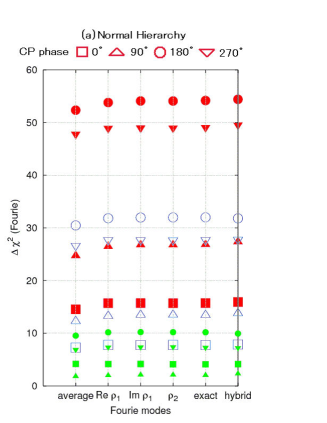
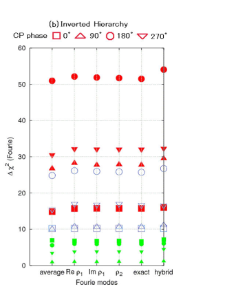
Figure 8: Minimum $\Delta\chi^{2}$ of the T2KK two detector experiment when the matter distribution along the baselines are approximated by their average, and up to first and second Fourier modes. They are compared with the results of the exact (step-function-like) matter distribution and those of the hybrid approximation to the oscillation probabilities. The input hierarchy is normal (inverted) in the plot a (b) where the opposite hierarchy is assumed in the fit. The input $\sin^{2}2\theta_{\rm RCT}$ are 0.10 for solid red, 0.06 for open blue, and 0.02 for solid green symbols, and the input CP phase are $0^{\circ}$ for squares, $90^{\circ}$ for upper triangles, $180^{\circ}$ for circle, and $270^{\circ}$ for upside-down triangles. The results are for $3.0^{\circ}$ OAB at SK, and for a 100 kt far detector at $L=1100$ km observing $1.0^{\circ}$ OAB, with the neutrino flux from $5\times 10^{21}$ POT at J-PARC.

In Fig. 8, we show the minimum values of $\Delta\chi^{2}$ for the T2KK two detector experiment as functions of the matter density distributions which are approximated by the distribution with the average density (average), including the real-part of the first Fourier mode (Re$\bar{\rho}_{1}$), further including the imaginary part (Im$\bar{\rho}_{1}$), and also with the second modes ($\bar{\rho}_{2}$). The results are then compared with $\Delta\chi^{2}_{\rm min}$ calculated by using the exact (step-function-like) distribution. As a reference, $\Delta\chi^{2}_{\rm min}$ calculated by the hybrid approximation of the oscillation probability, eq. (3.3), is also shown (hybrid). The input hierarchy is normal in the left figure while it is inverted in the right figure, where in both cases the opposite hierarchy is assumed in the fit. The input $\sin^{2}2\theta_{\rm RCT}$ is 0.10 for solid red blobs, 0.06 for open blue symbols, whereas 0.02 for solid green blobs, whereas the input CP phase are $0^{\circ}$ for squares, $90^{\circ}$ for upper triangles, $180^{\circ}$ for circle, and $270^{\circ}$ for upside-down triangles. We show the results for a far detector at $L=1100$ km baseline observing $1.0^{\circ}$ OAB, which has $-{\rm Re}(\bar{\rho}_{1})/\bar{\rho_{0}}=0.036$. Fig. 8 shows that the minimum $\Delta\chi^{2}$ values are reproduced accurately for all the cases just by accounting for the Re$(\bar{\rho}_{1})$ component. We conclude that higher Fourier modes including Im($\bar{\rho}_{1}$) do not affect the minimum $\Delta\chi^{2}$ significantly in the T2KK experiment.

The approximation of keeping only the linear term in Re$(\bar{\rho}_{1})$ in the oscillation probabilities, the hybrid method of section 3.3, works rather well at most cases. However, in Fig. 8(b), the hybrid method gives slightly high minimum $\Delta\chi^{2}$ for $\delta=180^{\circ}$ and $90^{\circ}$ at $\sin^{2}2\theta_{\rm RCT}=0.1$, and for $\delta=180^{\circ}$ at $\sin^{2}2\theta_{\rm RCT}=0.06$. In these cases, the hybrid method overestimates $\Delta\chi^{2}$ in bins around the oscillation minimum where the approximation is poor; see discussion in section 3.3. In more realistic studies including neutral current $\pi^{0}$ background, see ${\it e.g.}$ [20], those bins around the oscillation minima play less significant role due to the background dominance, and we expect that the hybrid method gives more reliable results.

5.2 Optimal T2KK setting for determining the mass hierarchy

Since the matter profile along the Tokai-to-Korea baseline depends on the baseline length as shown in Fig. 5, we re-examine the location dependence of the far detector capability to determine the neutrino mass hierarchy pattern. We show the result of our numerical calculation in Fig. 9,

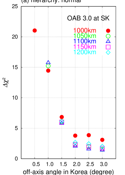
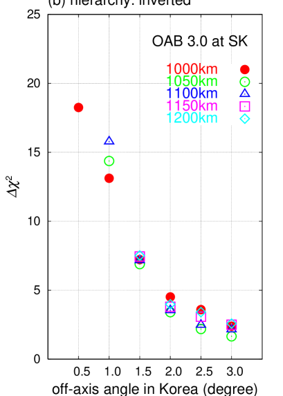
Figure 9: The minimum $\Delta\chi^{2}$ to exclude the wrong neutrino mass hierarchy as functions of the off-axis angle and the length of the far detector in Korea, when the $3.0^{\circ}$ OAB reaches SK. The left figure (a) for the normal hierarchy, and the right figure (b) is for the inverted hierarchy. The input parameters are the $|m^{2}_{3}-m^{2}_{1}|=2.35\times 10^{-3}{\rm eV}^{2}$, $m^{2}_{2}-m^{2}_{1}=8.3\times 10^{-3}{\rm eV}^{2}$, $\sin^{2}\theta_{\rm\footnotesize ATM}=0.5$, $\sin^{2}2\theta_{\rm\footnotesize SOL}=0.85$, $\sin^{2}2\theta_{\rm\footnotesize RCT}=0.10$ and $\delta_{\rm\footnotesize MNS}=0^{\circ}$. $\Delta\chi^{2}$ is calculated for a far detector for with 100 kt fiducial volume and for the neutrino flux with $5\times 10^{21}$ POT at J-PARC.

which shows the minimum $\Delta\chi^{2}$ to reject the wrong mass hierarchy for various combination of the off-axis angle and the baseline length of Tokai-to-Korea baseline, when the $3.0^{\circ}$ OAB reaches SK. The left figure (a) is for the normal hierarchy and the right figure (b) is for the inverted hierarchy. The input parameters are $|m^{2}_{3}-m^{2}_{1}|=2.35\times 10^{-3}{\rm eV}^{2}$, $m^{2}_{2}-m^{2}_{1}=7.5\times 10^{-3}{\rm eV}^{2}$, $\sin^{2}\theta_{\rm\footnotesize ATM}=0.5$, $\sin^{2}2\theta_{\rm\footnotesize SOL}=0.85$, $\sin^{2}2\theta_{\rm\footnotesize RCT}=0.10$ and $\delta_{\rm\footnotesize MNS}=0^{\circ}$, and $\Delta\chi^{2}$ is calculated for a far detector of 100 kt fiducial volume and $5\times 10^{21}$ POT at J-PARC. It should be noted here that the $0.5^{\circ}$ OAB reaches Korean peninsula only for $L\lower 2.15277pt\hbox{$\;\buildrel<\over{\sim}\;$}1030$ km; see the contour plot Fig. 1 of Ref. [17]. We therefore have only the $L=1000$ km point for $0.5^{\circ}$, three points for up to $L=1100$ km for $1.0^{\circ}$, all five points for higher off-axis angles in Fig. 9.

It is clear from the figure that the combination of OAB $0.5^{\circ}$ at $L=1000$ km is most powerful to determine the mass hierarchy pattern, for both the normal and inverted hierarchy cases. This is because the $0.5^{\circ}$ OAB has the strongest flux around the first oscillation maximum [18]. We also find that the $1.0^{\circ}$ OAB has significant sensitivity to the mass hierarchy especially at longer baseline lengths. The value of the $\Delta\chi^{2}$ for $1.0^{\circ}$ OAB at $L=1100$ km is 15.7 (15.8) for the normal (inverted) hierarchy, respectively, as compared to 21.0 (18.2) for $0.5^{\circ}$ OAB at $L=1000$ km. On the other hand, the sensitivity of T2KK experiment on the mass hierarchy decreases significantly for the off-axis angle greater than about $1.5^{\circ}$.

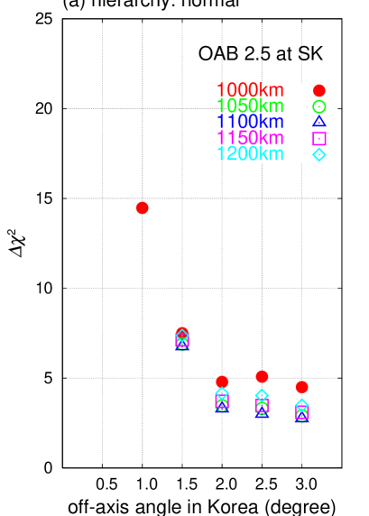
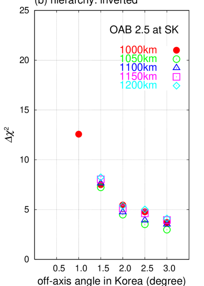
Figure 10: The same as Fig.9 but for the case when $2.5^{\circ}$ OAB reaches SK.

We also examin the case when the $2.5^{\circ}$ OAB reaches SK, whose results are shown in Fig. 10. It is worth noting here that no location inside Korean peninsula can observe the neutrino beam at an off-axis angle $\sim 0.5^{\circ}$ : See the off-axis angle contour plot of Fig 1 in Ref. [17]. The physical location of a far detector that detects $1.0^{\circ}$ OAB in Fig. 10 is the same as that of observing $0.5^{\circ}$ OAB in Fig. 9. In general, when we decreases the off-axis angle at SK by $0.5^{\circ}$, that of a far detector in Korea increases by $\sim 0.5^{\circ}$ as can be seen from the schematic picture of Fig. 1. Therefore, by comparing the minimum $\Delta\chi^{2}$ values of the corresponding points in Fig. 9 and 10, we can estimate the off-axis angle dependence of the T2KK experiment for each location of the far detector in Korea. We generally find that the minimum $\Delta\chi^{2}$ value decreases by about $40\%$ when the off-axis angle at SK is decreased from $3.0^{\circ}$ to $2.5^{\circ}$. It is therefore important that the off-axis angle at SK should be increased, i.e. the beam center should be oriented deeper into underground at J-PARC.

6 Earth matter effect for the anti-neutrino beam

In this section, we study the impacts of using the anti-neutrino beam in addition to the neutrino beam in the T2KK neutrino oscillation experiment.

Potential usefulness of having both neutrino and anti-neutrino beam run in the two detector experiments like T2KK can be understood as follows. The leading contributions to the $\nu_{\mu}\to\nu_{e}$ and $\bar{\nu}_{\mu}\to\bar{\nu}_{e}$ oscillation shifts in the amplitude and the phase are expressed, respectively, as

$$A^{e} \sim \pm\left(0.11\frac{\pi}{\Delta_{13}}\frac{L}{295{\rm km}}\frac{\bar{\rho}_{0}}{3{\rm g/cm}^{2}}-0.29\frac{\sin\delta}{\sqrt{y}}\right)\,,$$ (81a)

$$B^{e} \sim \mp 0.08\frac{L}{295{\rm km}}\frac{\bar{\rho}_{0}}{3{\rm g/cm}^{2}}+0.14\left(\frac{\cos\delta}{\sqrt{y}}-0.11\right)\,,$$ (81b)

where the upper signs are for $\nu_{\mu}\to\nu_{e}$ and the lower signs are for $\bar{\nu}_{\mu}\to\bar{\nu}_{e}$ oscillations, and only the leading terms in eq. (3.2) are kept. Because the matter effect terms proportional to $L\bar{\rho}_{0}$ contribute with opposite sign for $\nu_{\mu}$ and $\bar{\nu}_{\mu}$ oscillations, we can generally expect higher sensitivity to the mass hierarchy by comparing the oscillation probabilities at large $L$. In addition, since only the matter effect term changes the sign in the phase-shift term $B^{e}$ of eq. (81b), possible correlation between $\cos\delta$ and the mass hierarchy pattern can be resolved, and we can expect improvements in the hierarchy resolving power. On the other hand, since the $\bar{\nu}_{\mu}$ flux is generally lower than the $\nu_{\mu}$ flux for proton synchrotron based super beams, and also because the background level from the secondary $\nu_{e}$ flux is higher than the corresponding $\bar{\nu}_{e}$ background for the $\nu_{\mu}\to\nu_{e}$ signal, we should evaluate pros and cons quantitatively.

In order to estimate the merit of using both $\nu_{\mu}$ and $\bar{\nu}_{\mu}$ beams at T2KK, we repeat the $\Delta\chi^{2}$ analysis by assuming $2.5\times 10^{21}$ POT (2.5 years for the nominal T2K beam intensity [13]) each for $\nu_{\mu}$ and $\bar{\nu}_{\mu}$ beams, so that the total number of POT remains the same. We allow independent flux normalization errors of $3\%$ for the primary $\bar{\nu}_{\mu}$ beam, and the secondary $\bar{\nu}_{e},\nu_{\mu}$ and $\nu_{e}$ beams. The systematic error term of $\chi^{2}_{\rm sys}$ in eq. (71) now depends on 14 normalization factors;

$$\chi^{2~{}{\rm(new)}}_{\rm sys}=\chi^{2~{}(47)}_{\rm sys}+\sum_{\nu_{\alpha}=\bar{\nu}_{\mu},~{}\nu_{\mu},~{}\bar{\nu}_{e},~{}\nu_{e}}\left(\displaystyle\frac{\bar{f}_{\alpha}-1}{0.03}\right)^{2}\,,$$ (82)

where $\chi^{2~{}(47)}_{\rm sys}$ is defined in eq. (79), and the four $\bar{f}_{\alpha}$ terms measure the flux normalization uncertainty of the primary ($\bar{\nu}_{\mu}$) and the secondary ($\nu_{\mu},~{}\bar{\nu}_{e},~{}\nu_{e}$) fluxes in the anti-neutrino beam from J-PARC [18].

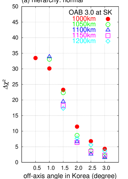
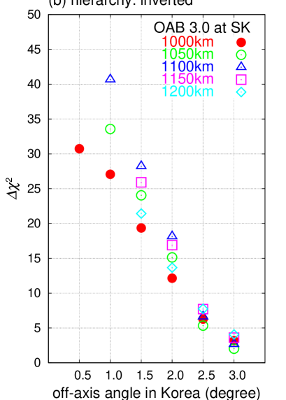
Figure 11: The same as Fig. 9 but when both neutrino and anti-neutrino beams are used. $\Delta\chi^{2}$ is calculated with $2.5\times 10^{21}$ POT for each beam so that their sum agrees with the neutrino flux assumed in Figs. 9 and 10.

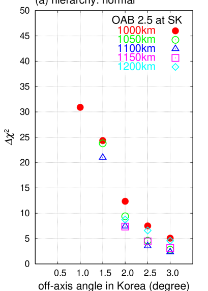
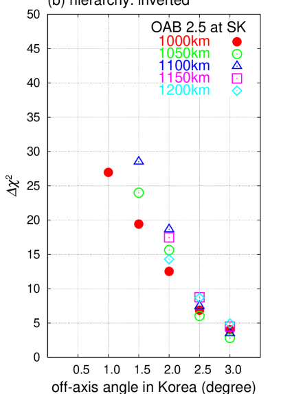
Figure 12: The same as Fig. 11, but the $2.5^{\circ}$ at SK.

The results are shown in Fig. 11 for $3.0^{\circ}$ OAB at SK, and Fig. 12 for the $2.5^{\circ}$ OAB at SK. It is remarkable that the splitting of the total neutrino flux into half $\nu_{\mu}$ and half $\bar{\nu}_{\mu}$ results in significant improvements in the mass hierarchy resolving power of the T2KK experiment. For the combination of $3.0^{\circ}$ OAB at SK and $0.5^{\circ}$ OAB at $L=1000$ km, the increase in $\Delta\chi^{2}_{\rm min}$ reads 21.0 to 33.4 for the normal hierarchy while 18.2 to 30.7 for the inverted hierarchy.

It is even more striking that the hierarchy resolving power at the 3 locations of the far detector at $1.0^{\circ}$ OAB is as high as that of $L=1000$ km at 0.5 OAB in Fig. 11. At $L=1100$ km (blue open triangles), $\Delta\chi^{2}_{\rm min}$ increases from 15.7 and 15.8 in Fig. 9, respectively, to 33.9 and 40.7 in Fig. 11 for the normal (a) and inverted (b) hierarchy case. We find that this is partly because of our choice of the CP phase, $\delta=0^{\circ}$. For $\cos\delta=1$ and $\sin^{2}2\theta_{\rm RCT}=0.1$, the phase-shift term $B^{e}$ in eq. (59b) becomes as large as 0.4 for the $\bar{\nu}_{\mu}\to\bar{\nu}_{e}$ oscillation, significantly shifting the peak location of eq. (34) to larger $|\Delta_{13}|$, or smaller $E_{\nu}$, for the inverted hierarchy ($\Delta_{13}<0$). This shift of the oscillation maximum to lower $E_{\nu}$ compensates for the slightly softer spectrum of the $1.0^{\circ}$ flux as compared to the $0.5^{\circ}$ OAB flux. We confirm the expected $\delta$ dependence of this observation by repeating the analysis for $\delta=180^{\circ}$, where the increase in $\Delta\chi^{2}_{\rm min}$ is not as dramatic as in the $\delta=0^{\circ}$ case. General survey of the physics capability of the T2KK experiment over the whole parameter space of the three neutrino model is beyond the scope of this report, and will be reported elsewhere.

We show in Fig. 12 the corresponding $\Delta\chi^{2}_{\rm min}$ values when the beam center is oriented upward by $0.5^{\circ}$ so that the $2.5^{\circ}$ OAB reaches SK, and hence the far detector in Korea observes the beam at $0.5^{\circ}$ larger off-axis angles. When we compare the $\Delta\chi^{2}_{\rm min}$ values in Figs. 11 and 12 at the same far detector locations, we generally find smaller values in Fig. 12, which are consequences of the softer neutrino beam spectra at larger off-axis angles. As in the neutrino beam only case, it is desirable to make the off-axis angle as large as possible at SK, so that the far detector in Korea can observe the same beam at a smaller off-axis angle.

7 Summary and discussion

In this paper, we study the earth matter effects in the T2KK experiment by using recent geophysical measurements [28, 29, 30, 31, 32].

The mean matter density $\bar{\rho}_{0}$ along the Tokai-to-Kamioka baseline is found to be $2.6{\rm g/cm}^{3}$. The presence of Fossa Magna along the T2K baseline makes the matter density distribution concave, or Re($\bar{\rho}_{1})>0$ for the first coefficient of the Fourier expansion of the density distribution along the baseline, which is opposite from what is naively expected from the spherically symmetric model of the earth matter distribution such as PREM [27]. We find that both the reduction of the average matter density $\bar{\rho}_{0}$ and the positive Re$(\bar{\rho}_{1})$ contribute positively to the mass hierarchy resolving power of the T2KK experiment, because the sensitivity grows as the difference in the magnitude of the earth matter effect between the oscillation probabilities observed at the near (SK) and a far (Korea) detectors.

As for the Tokai-to-Korea baselines, we find that the average matter density $\bar{\rho}_{0}$ grows from 2.85 g/cm³ at $L=1000$ km to 2.98 g/cm³ at $L=1100$ km, which are significantly higher than the PREM value of 2.70 g/cm³ ($L$ = 1000 km) and 2.78 g/cm³ ($L$ = 1100 km); see Table 2. This is essentially because both the Conrad discontinuity between the upper and the lower crust, and the Moho-discontinuity between the crust and the mantle are significantly higher than PREM in the main region of the baseline below the Japan/East sea. This also contributes positively to the mass hierarchy measurement. The distribution is convex as in PREM but Re$\bar{\rho}_{1}/\bar{\rho}_{0}$ is smaller in magnitude mainly becomes of the thin crust under the sea. One subtle point which we notice is that the $L=1000$ km baseline almost touches the Moho-discontinuity at its bottom, see Fig. 5, and hence small error in the depth of the discontinuity can change the average density significantly. If the Moho-discontinuity at about 20 km below the sea level is shallower by 0.7 km, which is the present error of the seismological measurement, $\bar{\rho}_{0}$ grows from 2.85 g/cm³ to 2.90 g/cm³, by about 2$\%$. On the other hand, this uncertainty does not affect the T2KK physics capability significantly because the major error in the earth matter density enters when the sound velocity data is converted to the matter density, for which we assign $6\%$ error in our analysis; see Fig. 3.

With the updated matter density distributions, we repeat the $\Delta\chi^{2}$ analysis of Refs. [17, 18], which estimates the mass hierarchy resolving power of the T2KK experiment, by performing a thought experiment with a far detector of 100 kt fiducial volume in various location of Korea along the T2K beam line. In order to perform the full parameter scan effectively, we introduce a new algorithm to compute the oscillation probabilities exactly for step-function-like matter density profile, where the earth matter effect is computed by diagonalizing real symmetric $3\times 3$ matrix by decoupling it from the evolution due to the $\theta_{23}$ mixing and the CP phase [34]. Analytic and semi-analytic approximations for the transition and survival probabilities are introduced to obtain physical interpretations of the numerical results.

We confirm the previous findings of Refs. [17, 18] that the mass hierarchy resolving capability is maximized when the T2K beam is oriented downward to $3.0^{\circ}$ OAB at SK and the far detector is placed in the south-east coast of Korean peninsula at $L\sim 1000$ km where $\sim 0.5^{\circ}$ OAB can be observed. In this report, we repeat the analysis by splitting the total beam time into half neutrino ($\nu_{\mu}$) and half anti-neutrino ($\bar{\nu}_{\mu}$) beams, and find significant improvements in the mass hierarchy resolving power. Most remarkably, we find that the highest level of sensitivity can now be achieved for a far detector in locations where the T2K neutrino beam can be detected at an off-axis angle up to $\sim 1^{\circ}$, because of the significant difference in the $E_{\nu}$-dependence of the oscillation probability between $\nu_{\mu}\to\nu_{e}$ and $\bar{\nu}_{\mu}\to\bar{\nu}_{e}$. This observation expands significantly the area in which a far detector can be most effective in determining the neutrino mass hierarchy pattern.
Acknowledgments
We thank our experimentalist colleagues Y. Hayato, A.K. Ichikawa, T. Kobayashi and T. Nakaya, from whom we learn about the K2K and T2K experiments. We thank N. Isezaki and M. Komazawa for teaching us about the geophysics measurements in Japan/East sea. We are also grateful to T. Kiwanami and M. Koike for useful discussions and comments. We thank the Aspen Center for Physics and the Phenomenology Institute at the University of Wisconsin for hospitality. The work is supported in part by the Grant in Aid for scientific research ($\#$20039014) from MEXT, and in part by the Core University Program of JSPS. The numerical calculations were carried out on KEKCC at KEK and Altix3700 BX2 at YITP in Kyoto University.

Appendix

In the appendix, we present the second order perturbation formula of the time-evolution operator for the location $(x)$ dependent Hamiltonian of eq. (3.2):

$$H(x) = H_{0}+\overline{H}_{1}+\delta H_{1}(x)\,,$$ (A.1)

where each term has the matrix element

$$\left\langle\nu_{\beta}\right|H_{0}\left|\nu_{\alpha}\right\rangle = \frac{m^{2}_{3}-m^{2}_{1}}{2E}U_{\beta 3}U^{*}_{\alpha 3}\,,$$ (A.2a)

$$\left\langle\nu_{\beta}\right|\overline{H}_{1}\left|\nu_{\alpha}\right\rangle = \frac{m^{2}_{2}-m^{2}_{1}}{2E}U_{\beta 2}U^{*}_{\alpha 2}+\frac{\bar{a}_{0}}{2E}\delta_{\beta e}\delta_{\alpha e}\,,$$ (A.2b)

$$\left\langle\nu_{\beta}\right|\delta H_{1}(x)\left|\nu_{\alpha}\right\rangle = \frac{1}{E}\sum^{\infty}_{k=1}\left[{\rm Re}(\bar{a}_{k})\cos\left(\frac{2\pi kx}{L}\right)+{\rm Im}(\bar{a}_{k})\sin\left(\frac{2\pi kx}{L}\right)\right]\delta_{\beta e}\delta_{\alpha e}\,.$$ (A.2c)

The first two terms, $H_{0}$ and $\overline{H}_{1}$, do not depend on the location $x$, whereas in the last term $\delta H_{1}(x)$ the $x$-dependent part of the matter density distribution along the baseline, $\rho(x)-\bar{\rho}_{0}$ is expressed as a Fourier expansion. The second term in eq. (A.2b) gives the matter effect due to the average matter density $\bar{\rho}_{0}$.

In the leading order, we consider only $H_{0}$ of eq. (A.2a). The time evolution via $H_{0}$ can readily be solved and the $\left|\nu_{\alpha}\right\rangle\to\left|\nu_{\beta}\right\rangle$ transition matrix element is

$$S_{0}(L)_{\beta\alpha} = \left\langle\nu_{\beta}\right|e^{-iH_{0}L}\left|\nu_{\alpha}\right\rangle=U_{\beta 1}U_{\alpha 1}^{*}+U_{\beta 2}U_{\alpha 2}^{*}+U_{\beta 3}U_{\alpha 3}^{*}e^{-i\Delta_{13}}$$ (A.3)

$$= \delta_{\beta\alpha}+U_{\beta 3}U_{\alpha 3}^{*}\left(e^{-i\Delta_{13}}-1\right)\,,$$

with $\Delta_{13}$ as in eq. (48). In the next order, we divide the corrections into two parts,

$$S_{1}(L)_{\beta\alpha} = S_{1}^{(1)}(L)_{\beta\alpha}+S_{1}^{(2)}(L)_{\beta\alpha}\,,$$ (A.4)

where the first term is linear in $\bar{H}_{1}$;

$$S_{1}^{(1)}(L)_{\beta\alpha} = -i\left\langle\nu_{\beta}\right|\left(\int^{L}_{0}dxe^{iH_{0}(x-L)}\bar{H}_{1}e^{-iH_{0}x}\right)\left|\nu_{\alpha}\right\rangle$$ (A.5)

$$= -i\Delta_{12}U_{\beta 2}U_{\alpha 2}^{*}-i\frac{\bar{a}_{0}L}{2E}\biggl{[}\delta_{\beta e}\delta_{\alpha e}-A_{\beta\alpha}+2B_{\beta\alpha}\biggr{.}$$

$$+\left.\left(e^{-i\Delta_{13}}-1\right)\left\{B_{\beta\alpha}+\frac{i}{\Delta_{13}}\left(A_{\beta\alpha}-2B_{\beta\alpha}\right)\right\}\right]\,,$$

and the second term is linear in $\delta H_{1}$.

$$S_{1}^{(2)}(L)_{\beta\alpha} = -i\left\langle\nu_{\beta}\right|\left(\int^{L}_{0}dxe^{iH_{0}(x-L)}\delta H_{1}(x)e^{-iH_{0}x}\right)\left|\nu_{\alpha}\right\rangle$$ (A.6)

$$= \frac{L}{E}\frac{e^{-i\Delta_{13}}-1}{\Delta_{13}}\times$$

$$\sum^{\infty}_{k=1}\left[\frac{{\rm Re}(\bar{a}_{k})\Delta_{13}^{2}}{\Delta_{13}^{2}-\left(2\pi k\right)^{2}}\left(A_{\beta\alpha}-2B_{\beta\alpha}\right)-i\frac{{\rm Im}(\bar{a}_{k})2\pi k\Delta_{13}}{\Delta_{13}^{2}-\left(2\pi k\right)^{2}}C_{\beta\alpha}\right]\,.$$

Here the coefficients $A_{\beta\alpha}$, $B_{\beta\alpha}$, and $C_{\beta\alpha}$ are quadratic terms of the MNS matrix elements,

$$A_{\beta\alpha} \equiv \delta_{\beta e}U_{e3}U_{\alpha 3}^{*}+U_{\beta 3}U_{e3}^{*}\delta_{\alpha e}\,,$$ (A.7a)

$$B_{\beta\alpha} \equiv U_{\beta 3}U_{\alpha 3}^{*}|U_{e3}|^{2}\,,$$ (A.7b)

$$C_{\beta\alpha} \equiv \delta_{\beta e}U_{e3}U_{\alpha 3}^{*}-U_{\beta 3}U_{e3}^{*}\delta_{\alpha e}\,.$$ (A.7c)

Generally, the $B_{\beta\alpha}$ terms are much smaller than the other terms because of the constraint $|U_{e3}|^{2}<0.044$. Since $A_{\mu\mu}=0$ and $|B_{\mu\mu}|\sim|U_{\mu 3}U_{e3}|^{2}\ll 1$, we can approximate $S^{(1)}_{1}(L)_{\mu\mu}$ rather accurately by $-i\Delta_{12}|U_{\mu 2}|^{2}$, which does not depend on the matter effect term $\bar{a}_{0}$. On the other hand, $|A_{e\mu}|$ can be as large as $|U_{\mu 2}U_{e2}|$ in $S_{1}^{(1)}(L)_{e\mu}$, and the matter effect can be significant.

As for the $x$-dependent perturbation $S^{(2)}_{\beta\alpha}$, we note that the terms proportional to Re$(\bar{a}_{k})$ are in phase with the leading term of eq. (A.3) for $\beta\alpha=e\mu$, whereas those with Im$(\bar{a}_{k})$ are orthogonal. Therefore the Im$(\bar{a}_{k})$ terms contribute to the $\nu_{\mu}\to\nu_{e}$ oscillation probability only as Im$(\bar{a}_{k})^{2}|C_{e\mu}|^{2}\sim(\bar{a}_{k})^{2}|U_{e3}|^{2}$, which is strongly suppressed. Contributions to the $\nu_{\mu}\to\nu_{\mu}$ survival probability are strongly suppressed again in this order due to the smallness of $|A_{\mu\mu}-2B_{\mu\mu}|$ and $C_{\mu\mu}=0$.

Finally, the second order correction, $S_{2}$, is evaluated only for $x$-independent perturbation, $\overline{H}_{1}$, because the magnitude of all the non-zero Fourier coefficients are significantly smaller than the average, $\bar{\rho}_{0}$; see Figs. 4, 6 and Table 2. We find

$$S_{2}(L)_{\beta\alpha} = -\left\langle\nu_{\beta}\right|\left(\int^{L}_{0}dx\int^{x}_{0}dye^{iH_{0}(x-L)}\overline{H}_{1}e^{iH_{0}(y-x)}\overline{H}_{1}e^{-iH_{0}y}\right)\left|\nu_{\alpha}\right\rangle$$ (A.9)

$$= -i\sum_{\gamma}\int^{L}_{0}dx\left[\frac{\Delta_{12}}{L}U_{\beta 2}U_{\gamma 2}^{*}+\frac{\bar{a}_{0}}{2E}\left\{\delta_{\beta e}\delta_{e\gamma}+U_{\beta 3}U_{e3}^{*}\delta_{e\gamma}\left(e^{i\frac{\Delta_{13}}{L}(x-L)}-1\right)\right\}\right]S_{1}^{(1)}(x)_{\gamma\alpha}$$

$$= -\frac{\Delta_{12}^{2}}{2}U_{\beta 2}U_{\alpha 2}^{*}$$

$$-\frac{\Delta_{12}}{2}\frac{\bar{a}_{0}L}{2E}\left[D_{\beta\alpha}-\left\{1+\frac{2i}{\Delta_{13}}+\frac{2\left(e^{-i\Delta_{13}}-1\right)}{\Delta_{13}^{2}}\right\}E_{\beta\alpha}\right]$$

$$-\left(\frac{\bar{a}_{0}L}{2E}\right)^{2}\left[\frac{1}{2}\left\{\left(1-|U_{e3}|^{2}\right)\left(\delta_{\beta e}\delta_{\alpha e}-A_{\beta\alpha}\right)+B_{\beta\alpha}\right\}\right.$$

$$\hskip 31.2982pt\left.-\frac{i}{\Delta_{13}}\left\{\delta_{\beta e}\delta_{\alpha e}|U_{e3}|^{2}+\left(1-3|U_{e3}|^{2}\right)A_{\beta\alpha}-3\left(1-2|U_{e3}|^{2}\right)B_{\beta\alpha}\right\}\right.$$

$$\hskip 31.2982pt\left.+\left(e^{-i\Delta_{13}}-1\right)\left\{\frac{1}{2}|U_{e3}|^{2}B_{\beta\alpha}+\frac{i}{\Delta_{13}}\left(|U_{e3}|^{2}A_{\beta\alpha}+\left(1-3|U_{e3}|^{2}\right)B_{\beta\alpha}\right)\right.\right.$$

$$\hskip 31.2982pt\left.\left.+\frac{1}{\Delta_{13}^{2}}\left(-\delta_{\beta e}\delta_{\alpha e}|U_{e3}|^{2}-\left(1-3|U_{e3}|^{2}\right)A_{\beta\alpha}+3\left(1-2|U_{e3}|^{2}\right)B_{\beta\alpha}\right)\right\}\right]\,,$$

where $D_{\beta\alpha}$ and $E_{\beta\alpha}$ are the MNS matrix element factors

$$D_{\beta\alpha} = \delta_{\beta e}U_{e2}U_{\alpha 2}^{*}+U_{\beta 2}U_{e2}^{*}\delta_{\alpha e}\,,$$ (A.10a)

$$E_{\beta\alpha} = U_{\beta 2}U_{e2}^{*}U_{e3}U_{\alpha 3}^{*}+U_{\beta 3}U_{e3}^{*}U_{e2}U_{\alpha 2}^{*}\,.$$ (A.10b)

It should be noted that although $\Delta_{12}^{2}$ is small, $0.01$, around the first oscillation maximum $|\Delta_{13}|\sim\pi$, it is significant around the second oscillation maximum $|\Delta_{13}|\sim 3\pi$ where it grows to $0.1$. The combination, $\Delta_{12}(\bar{a}_{0}L/2E)$ is about 0.02 for T2K and 0.06 for $L\sim 1000$ km around $|\Delta_{13}|\sim\pi$. The matter effect term squared, $(\bar{a}_{0}L/2E)^{2}$, is 0.03 at Kamioka while it grows to $\sim 0.3$ or larger for the Tokai-to-Korea baselines.

References

- [1] Z. Maki, M. Nakagawa, and S. Sakata, Prog. Theor. Phys. 28, 870 (1962).
- [2] Y. Fukuda et al. [Super-Kamiokande Collaboration], Phys. Rev. Lett. 81, 1562 (1998) [hep-ex/9807003]; Y. Ashie et al. [Super-Kamiokande Collaboration], Phys. Rev. D71, 112005 (2005) [hep-ex/0501064].
- [3] M. Ambrosio et al. [MACRO Collaboration], Phys. Lett. B566 35 (2003) [hep-ex/0304037]; M. C. Sanchez et al. [Soudan 2 Collaboration], Phys. Rev. D68, 113004 (2003) [hep-ex/0307069].
- [4] M. H. Ahn et al. [K2K collaboration], Phys. Rev. D 74, 072003 (2006) [hep-ex/0606032].
- [5] P. Adamson et al. [MINOS Collaboration], Phys. Rev. D73, 072002 (2006) [hep-ex/0512036].
- [6] M. B. Smy et al. [Super-Kamiokande Collaboration], Phys. Rev. D69, 011104 (2004) [hep-ex/0309011]; B. Aharmim et al. [SNO Collaboration], Phys. Rev. C 72, 055502 (2005) [nucl-ex/0502021].
- [7] A. Gando et al. [The KamLAND Collaboration], Phys. Rev. D 83, 052002 (2011)[arXiv:1009.4771 [hep-ex]].
- [8] M. Apollonio et al., Eur. Phys. J. C27 331 (2003) [hep-ex/0301017].
- [9] F. Boehm et al., Phys. Rev. Lett. 84, 3764 (2000) [hep-ex/9912050].
- [10] The Double-CHOOZ Collaboration [hep-ex/0405032]; M. G. T. Lasserre,[hep-ex/0606025].
- [11] J. K. Ahn et al. [RENO Collaboration], [arXiv:1003.1391 [hep-ex]].
- [12] X. Guo et al. [Daya Bay Collaboration], [hep-ex/0701029]
- [13] Y. Itow et al., [hep-ex/0106019]. see also the T2K official home page, http://jnusrv01.kek.jp/public/t2k/.
- [14] D. S. Ayres et al. [NOvA Collaboration] [hep-ex/0503053].
- [15] K. Hagiwara, Nucl. Phys. Proc. Suppl. 137, 84 (2004) [hep-ph/0410229].
- [16] M. Ishitsuka, T. Kajita, H. Minakata, and, H. Nunokawa, Phys. Rev. D72, 033003 (2005) [hep-ph/0504026].
- [17] K. Hagiwara, N. Okamura, and K. Senda, Phys. Lett. B637 266 (2006) [Erratum ibid.B641 486 (2006)] [hep-ph/0504061].
- [18] K. Hagiwara, N. Okamura, and K. Senda, Phys. Rev. D 76, 093002 (2007) [hep-ph/0607255].
- [19] K. Hagiwara and N. Okamura, JHEP 0801, 022 (2008) [hep-ph/0611058].
- [20] K. Hagiwara and N. Okamura, JHEP 0907, 031 (2009) [arXiv:0901.1517 [hep-ph]].
- [21] L. Wolfenstein, Phys. Rev. D17, 2369 (1978); R.R. Lewis, ibid. 21, 663 (1980); V. Barger, S. Pakvasa, R.J.N. Phillips and K. Whisnant, ibid. 22, 2718 (1980); S.P. Mikheyev and A.Yu. Smirnov, Yad. Fiz. 42, 1441 (1985) [Sov.J.Nucl.Phys. 42, 913 (1986)]; Nuovo Cimento C9, 17 (1986).
- [22] T. Takeda et al., Earth Planets Space, 56, 1293, (2004).
- [23] M. Koike and J. Sato, Mod. Phys. Lett. A 14, 1297 (1999) [hep-ph/9803212].
- [24] Geological Sheet Map 1:500,000 No. 8 TOKYO ( 2nd ed., 2nd print); Fig. 1 in Ref. [23].
- [25] J-PARC home page, http://j-parc.jp/.
- [26] W.J. Ludwig, J. E. Nafe. and C. L. Drake, ‘Seismic Refraction, in the sea.’ Edited by A. E. Maxwell, Wiley-Interscience, New York.
- [27] A.M. Dziewonski and D.L. Anderson, Phys. Earth Planet. Interiors 25, 297 (1981).
- [28] T. Sato et al., Geochem. Geophys. Geosyst. 7, Q06004, (2006) .
- [29] T. Sato et al., Tectonophys. 412, 159, (2006).
- [30] H. J. Kim et al., Tectonophys. 364, 25 (2003).
- [31] D. Zhao, S. Horiuchi, and A. Hasegawa, Tectonophys. 212 389 (1992).
- [32] H.M. Cho et al., Geophys. Res. Lett. 33, L06307 (2006)].
- [33] T. Ohlsson and H. Snellman, J. Math. Phys. 41, 2768 (2000) [Erratum-ibid. 42, 2345 (2001)] [hep-ph/9910546]; Phys. Lett. B 474, 153 (2000) [hep-ph/9912295]; E. K. Akhmedov et al., JHEP 0404, 078 (2004) [arXiv:hep-ph/0402175].
- [34] K. Kimura, A. Takamura, and H. Yokomakura, Phys. Lett. B544, 286 (2002) [hep-ph/0203099]; Phys. Rev. D 66, 073005 (2002) [hep-ph/0205295].
- [35] A.K. Ichikawa, private communication; the flux data for various off-axis angles are available from the web page; http://www2.yukawa.kyoto-u.ac.jp/~okamura/T2KK/.
- [36] R. A. Smith and E. J. Moniz, Nucl. Phys. B 43, 605 (1972) [Erratum ibid. B 101, 547 (1975)].
- [37] K. Abe et al. [T2K Collaboration], Phys. Rev. Lett. 107, 041801 (2011) [arXiv:1106.2822 [hep-ex]].
- [38] P. Adamson et al. [MINOS Collaboration], [arXiv:1108.0015 [hep-ex]].