Auxiliary Field quantum Monte Carlo for Strongly Paired Fermions

Abstract

We demonstrate that the inclusion of a BCS importance function dramatically increases the efficiency of the auxiliary field method for strong pairing. We calculate the ground-state energy of an unpolarized fermi gas at unitarity with up to 66 particles and lattices of up to $27^{3}$ sites. The method has no fermion sign problem, and an accurate result is obtained for the universal parameter $\xi$. Several different forms of the kinetic energy adjusted to the unitary limit but with different effective ranges extrapolate to the same continuum limit within error bars. The finite effective range results for different interactions are consistent with a linear term proportional to the Fermi momentum times the effective range. The new method described herein will have many applications in superfluid cold atom systems and in both electronic and nuclear structures when pairing is important.

The study of strongly interacting Fermi systems is one of the central themes and major challenges in physics. Superfluidity in unpolarized cold atomic Fermi gases, which has been demonstrated both experimentally and theoretically, provides a prototypical example. The experimental ability to use a Feshbach resonance to adjust the strength of the potential between the atoms allows an exploration of the physics over many length scales. A particularly interesting regime is at unitarity where the scattering length diverges and the range of the potential can be neglected. Since the particle density provides the only length scale, the ground-state energy $E_{0}$ is proportional to the free fermi gas energy $E_{FG}$,

$$E_{0}=\xi E_{FG}\,.$$ (1)

The ability to quantitatively understand the properties of this system represents a great triumph of many-body physics. Many experiments and calculations have been performed for the unitary Fermi gas. Initial qualitative agreement was found between theoryCarlson:2003 ; *Chang:2004; Astrakharchik:2004 and experimentBartenstein:2004 ; Kinast:2005 ; Partridge:2006 . More precise recent experiments have yielded $\xi=0.39(2)$Luo:2009 and $0.41(1)$Navon:2010 , with smaller values obtained very recently by Zwierlein, et al.Zwierlein:2011 . Fixed-node Diffusion Monte Carlo (DMC) calculationsCarlson:2003 ; *Chang:2004; Astrakharchik:2004 ; Carlson:2005 ; Lobo:2006 ; Forbes:2011 ; Gandolfi:2011 have always included a Bardeen-Cooper-SchriefferBardeen:1957 (BCS) trial wave function to guide the Monte Carlo walk and provide the fixed node constraintAnderson:1976 needed to overcome the fermion sign problem. As is well known, these calculations provide an upper bound, with the current best value $\xi=0.383(1)$Forbes:2011 ; Gandolfi:2011 .

In this paper we show that exact calculations can be performed to accurately determine the ground-state properties of the unpolarized Fermi gas. A new method is introduced to allow the use of a BCS trial wave function in the auxiliary-field quantum Monte Carlo (AFQMC) approaches of Zhang and coworkersZhang:1995 ; *Zhang:1997; Zhang:2003 . Using the new approach, we perform calculations with several forms of the kinetic energy term that all give the correct continuum limit but with different finite effective ranges to study the convergence with particle number and lattice sizes, and to obtain the dependence of $\xi$ on the effective range. An exact result is obtained for the value of $\xi$.

Quantum Monte Carlo simulations play a key role in addressing the challenge of strongly interacting Fermi systems. The AFQMC method has been applied to a variety of systems in several fields. With equal numbers and masses of up- and down-spin fermions and an attractive interaction, there is no fermion sign problem. The formalism presented here allows the use of a BCS importance function, which drastically improves the efficiency in this situation. In general applications, a sign or phase problem is present, which is controlled by a constraint, also using the importance function Zhang:1995 ; *Zhang:1997; Zhang:2003 . Hartree-Fock or free Fermi gas (FG) type of importance functions have typically been used. This approach has been shown to be very accurate in many condensed matter models and optical lattices PhysRevLett.104.116402 , quantum chemistry al-saidi:224101 , and solid state materials PhysRevB.80.214116 . Now BCS importance functions (or antisymmetrized geminal power (AGP) in chemistry) will significantly improve our ability to deal with the sign problem in systems where pairing is important, and enhance the capabilities for quantum simulations in strongly correlated systems in general.

The AFQMC method, in both-zeroLee:2006 and finite-temperature formulationsBulgac:2006 , has also been applied to the unitary Fermi gas. Precise results require simultaneously large lattices, so the system is dilute, and a large number of particles for an accurate approach to the continuum and thermodynamic limits. Many such calculations have been performedLee:2006 ; Lee:2007 ; Lee:2008a ; Lee:2008b ; Bour:2011 , but the variance of the method limited the results to relatively small number of particles and lattice sizes so that, as we demonstrate below, the results are unlikely to have converged to the thermodynamic limit.

The range of the van der Waals interaction in cold atoms is small (e.g. about 3 nm in ⁶LiKetterle:2008 ) compared to interparticle spacing so that the short range structure of the interaction is unimportant; the results are completely determined by the form of the kinetic energy and the scattering length. For an $N_{k}^{3}$ lattice, the equivalent Hamiltonian is

$$H=\frac{1}{N_{k}^{3}}\sum_{\boldsymbol{k},\boldsymbol{j},\boldsymbol{m},s}\psi^{\dagger}_{\boldsymbol{j}s}\psi_{\boldsymbol{m}s}\epsilon_{\boldsymbol{k}}e^{i\boldsymbol{k}\cdot(\boldsymbol{r}_{\boldsymbol{j}}-\boldsymbol{r}_{\boldsymbol{m}})}+U\sum_{\boldsymbol{i}}n_{\boldsymbol{i}\uparrow}n_{\boldsymbol{i}\downarrow}\,.$$ (2)

Here $\psi_{\boldsymbol{j}s}$ is the destruction operator for a fermion of spin $s$ on lattice site at position $\boldsymbol{r}_{\boldsymbol{j}}$. For odd lattice sizes $N_{k}=2N_{c}+1$, the $\boldsymbol{k}$ are given by $\frac{2\pi}{L}(n_{x}{\boldsymbol{\hat{x}}}+n_{y}{\boldsymbol{\hat{y}}}+n_{z}{\boldsymbol{\hat{z}}})$ with $-N_{c}\leq n_{x},n_{y},n_{z}\leq N_{c}$. The $k$ space destruction operators are $c_{\boldsymbol{k}s}=N_{k}^{-3/2}\sum_{\boldsymbol{j}}e^{-i\boldsymbol{k}\cdot\boldsymbol{r}_{\boldsymbol{j}}}\psi_{\boldsymbol{j}s}$, and the density operators are $n_{\boldsymbol{i}s}=\psi^{\dagger}_{\boldsymbol{i}s}\psi_{\boldsymbol{i}s}$.

To reach the continuum limit, we need to take the limit of zero particle density, $\rho\equiv N/N_{k}^{3}\rightarrow 0$, in the context of the Hubbard model (i.e., replace $L$ by $N_{k}$). Equivalently, because of scale invariance, we can think of the system as a discretized representation of a supercell with fixed size $L$, and take the $k$-space cutoff to infinity. In either case, we then take the number of particles, $N$, to infinity. In this limit only the behavior of $\epsilon_{k}$ for $k\ll\frac{2\pi}{\alpha}$ is important, where $\alpha\equiv L/N_{k}$ is the lattice spacing. Thus a variety of kinetic energy forms can be used as long as they are quadratic for $k$ much smaller than the cutoff. In this work we present results for

$$\epsilon^{(2)}_{k} = \frac{\hbar^{2}k^{2}}{2m}\,,\ \ \epsilon^{(4)}_{k}=\frac{\hbar^{2}k^{2}}{2m}\left[1-\beta^{2}k^{2}\alpha^{2}\right]$$

$$\epsilon^{(h)}_{\boldsymbol{k}} = \frac{\hbar^{2}}{m\alpha^{2}}\left[3-\cos(k_{x}\alpha)-\cos(k_{y}\alpha)-\cos(k_{z}\alpha)\right]\,.$$ (3)

The superscript $2$ and $4$ indicate the highest power of $k$, while $\epsilon^{(h)}$ is the Hubbard model hopping kinetic energy offset by a constant so that it is zero at $\boldsymbol{k}=0$.

For two particles, the Hamiltonian is separable, and the solution of the Lippmann-Schwinger equation for low-energy s-wave scattering gives the phase-shift equation,

$$\begin{split}&k\cot\delta_{0}=-\frac{4\pi\hbar^{2}}{mU\alpha^{3}}\left[\rule[-11.38109pt]{2.84526pt}{0.0pt}1+\right.\\ &\left.\frac{U\alpha^{3}}{16\pi^{3}}{\cal P}\int_{-\pi/\alpha}^{\pi/\alpha}dk_{x}^{\prime}\int_{-\pi/\alpha}^{\pi/\alpha}dk_{y}^{\prime}\int_{-\pi/\alpha}^{\pi/\alpha}dk_{z}^{\prime}\frac{1}{\epsilon_{\boldsymbol{k}^{\prime}}-\epsilon_{\boldsymbol{k}}}\right]\end{split}$$ (4)

where ${\cal P}$ indicates the principal parts integration, and the $k$ space sums are cut off by the lattice spacing $\alpha$. The effective range expansion is

$$k\cot\delta_{0}=-a^{-1}+\tfrac{1}{2}k^{2}r_{e}+...$$ (5)

where $a$ is the scattering length and $r_{e}$ the effective range. Since we are interested in the unitary limit, we adjust $U$ to have $a^{-1}=0$. Both $\epsilon^{(2)}_{k}$ and $\epsilon^{(h)}_{\boldsymbol{k}}$ have nonzero effective ranges. The extra parameter $\beta$ in $\epsilon^{(4)}_{k}$ can be adjusted to make the effective range zero. The values for the parameters are given in table 1.

Energy	$U\tfrac{2m\alpha^{2}}{\hbar^{2}}$	$\beta$	$r_{e}\alpha^{-1}$
$\epsilon^{(h)}_{\boldsymbol{k}}$	-7.91355	-	-0.30572
$\epsilon^{(2)}_{k}$	-10.28871	-	0.33687
$\epsilon^{(4)}_{k}$	-8.66605	0.16137	0.00000

Table 1: The parameters that give infinite scattering length for two particles in an infinite lattice for the various kinetic energies. The $\beta$ value for the $\epsilon^{(4)}_{k}$ kinetic energy has been adjusted to give zero effective range, $r_{e}$.

The AFQMC algorithm uses branching random walks to project the ground state from an initial trial state with the imaginary-time operator $\exp[-H\tau]$. Because the interaction is attractive, there is no fermion sign problem for equal numbers of up and down fermions studied here, and no path constraint is required. A walker is a set of $N$ single-particle orbitals. Initially, the orbitals for the up spin particles are taken to be identical to those for the down spin particles. The two-body interaction term is broken up using a Hubbard-Stratonovich (HS) transformation which has only positive weights, and treats the up and down spin particles identically. Therefore, the up spin orbitals remain identical to the down spin orbitals during the propagation. We will show below that the usual form for a singlet paired BCS trial function also gives no fermion sign problem.

The walker states are given by specifying the orbital coefficients. These can be specified on the real space lattice $\phi_{n,\boldsymbol{j}}$ or as momentum space coefficients $\tilde{\phi}_{n,\boldsymbol{k}}$ related to each other by a discrete Fourier transform. If we begin with real orbitals on the real space lattice, the orbitals remain real when propagated. The momentum space orbitals therefore satisfy $\tilde{\phi}_{n,-\boldsymbol{k}}=\tilde{\phi}_{n,\boldsymbol{k}}^{*}$. The orbitals are orthonormalized at each step. This is needed to limit roundoff error, but the mathematical expressions are correct without it. The orthonormal orbitals therefore satisfy $\sum_{\boldsymbol{k}}\tilde{\phi}_{n,\boldsymbol{k}}^{*}\tilde{\phi}_{m,\boldsymbol{k}}=\delta_{nm}$, and the corresponding operators, $w_{ns}=\sum_{k}\tilde{\phi}_{n,\boldsymbol{k}}c_{\boldsymbol{k}s}$, satisfy $\{w_{ns},w^{\dagger}_{ms^{\prime}}\}=\delta_{nm}\delta_{ss^{\prime}}$. The walker state is

$$|W\rangle = \prod_{n=1}^{N/2}w^{\dagger}_{n\uparrow}w^{\dagger}_{n\downarrow}|0\rangle\,.$$ (6)

Because $N\ll N_{k}^{3}$ and because the imaginary-time history of the walk need not be retained, this formalism is much more efficient than the usual lattice formulations for the ground state of dilute gases.

Using a discrete HS transformationHirsch:1983 , the potential energy propagator is

$$\begin{split}&e^{-U\sum_{i}n_{\boldsymbol{i}\uparrow}n_{\boldsymbol{i}\downarrow}\Delta t}=\frac{1}{2^{N_{k}^{3}}}\sum_{\{\sigma\}=\pm 1}G_{V}(\{\sigma\},\Delta t)\\ &G_{V}(\{\sigma\},\Delta t)=\exp\left[\sum_{\boldsymbol{i},s}\left(2u\sigma_{\boldsymbol{i}}-\tfrac{1}{2}U\Delta t\right)n_{\boldsymbol{i}s}-u\sigma_{\boldsymbol{i}}\right]\\ \end{split}$$ (7)

where $\tanh^{2}u=-\tanh\left(\frac{U\Delta t}{4}\right)$. The kinetic energy propagator is

$$G_{T}(\Delta t)=\exp\left[-\sum_{\boldsymbol{k}}\epsilon_{\boldsymbol{k}}\left(c^{\dagger}_{\boldsymbol{k}\uparrow}c_{\boldsymbol{k}\uparrow}+c^{\dagger}_{\boldsymbol{k}\downarrow}c_{\boldsymbol{k}\downarrow}\right)\Delta t\right]\,.$$ (8)

Given a choice of one of the $N_{k}^{3}$ set of fields, the application of the Trotter breakup of one term of the propagator on a walker $|W\rangle$ gives another walker $|W^{\prime}\rangle$ times a weight $w^{\prime}(\{\sigma\},W)$ that depends on the set of HS variables $\{\sigma\}$ and $|W\rangle$,

$$G(\{\sigma\},\Delta t)|W\rangle \equiv G_{T}(\tfrac{\Delta t}{2})G_{V}(\{\sigma\},\Delta t)G_{T}(\tfrac{\Delta t}{2})|W\rangle$$ (9)

$$\rightarrow w^{\prime}(\{\sigma\},W)|W^{\prime}\rangle\,.$$

The propagation above consists of (1) Multiply each $\tilde{\phi}_{n,\boldsymbol{k}}$ by $\exp(-\tfrac{1}{2}\epsilon_{\boldsymbol{k}}\Delta t)$. (2) Fast Fourier transform to obtain $\phi_{n,\boldsymbol{i}}$ in real space. (3) Multiply each $\phi_{n,\boldsymbol{i}}$ by $\exp\left(2u\sigma_{i}-\tfrac{1}{2}U\Delta t\right)$. (4) Fast Fourier transform to obtain $\tilde{\phi}_{n,\boldsymbol{k}}$ in momentum space. (5) Multiply each $\tilde{\phi}_{n,\boldsymbol{k}}$ by $\exp(-\tfrac{1}{2}\epsilon_{\boldsymbol{k}}\Delta t)$. (6) Update the weight from non-operator terms.

Including importance sampling reduces the fluctuations, by changing the sampling so that it is non-uniform, without biasing the results. We want to sample walkers $|W\rangle$ from $\langle\Psi_{T}|W\rangle\langle W|\psi(t)\rangle$ where

$$|\psi(t+\Delta t)\rangle=e^{-(H-E_{T})\Delta t}|\psi(t)\rangle$$ (10)

The contribution of a walker $|W\rangle$ at the next time step is then

$$\begin{split}&\sum_{\{\sigma\}=\pm 1}\left[\frac{1}{2^{N_{k}^{3}}}\frac{\langle\Psi_{T}|G(\{\sigma\},\Delta t)|W\rangle}{\langle\Psi_{T}|W\rangle}e^{-E_{T}\Delta t}\right]\times\\ &\ \ \ \ \ \frac{1}{w(\{\sigma\},W)}G(\{\sigma\},\Delta t)|W\rangle\,.\end{split}$$ (11)

We want to sample the set of HS variables $\{\sigma\}$, from the unnormalized probability distribution given by the square brackets. The normalization which, to order $\Delta t^{2}$ is the local energy expression $e^{-(\tfrac{1}{2}[E_{L}(W)+E_{L}(W^{\prime})]-E_{T})\Delta t}$, will give the weight of the sampled walkers. Once we have sampled the $\{\sigma\}$ values, the new normalized walker is given by the second term of Eq. 11. We make sure that regions where the trial function is small are sampled adequately to eliminate trial-function bias.

The particle projected BCS state is

$$|BCS\rangle=\left[\sum_{\boldsymbol{k}}f_{k}c^{\dagger}_{\boldsymbol{k}\uparrow}c^{\dagger}_{-\boldsymbol{k}\downarrow}\right]^{N/2}|0\rangle\,,$$ (12)

where $f_{k}=v_{k}/u_{k}$ in the usual notation. The overlap of a walker with the BCS state is

$$\langle W|BCS\rangle=\langle 0|\prod_{n=1}^{N/2}w_{n\downarrow}w_{n\uparrow}\left[\sum_{\boldsymbol{k}}f_{k}c^{\dagger}_{\boldsymbol{k}\uparrow}c^{\dagger}_{-\boldsymbol{k}\downarrow}\right]^{N/2}|0\rangle$$ (13)

The contraction needed is $\mathchoice{\vbox{\hbox to0.0pt{\kern 0.0pt\kern 3.71413pt\hbox{\vrule width=0.50003pt,height=0.0pt,depth=4.30554pt\vrule width=12.7442pt,height=0.0pt,depth=0.50003pt\vrule width=0.50003pt,height=0.0pt,depth=4.30554pt}\hss}\vskip 2.15277pt\vskip 4.30554pt}}{\vbox{\hbox to0.0pt{\kern 0.0pt\kern 3.71413pt\hbox{\vrule width=0.50003pt,height=0.0pt,depth=4.30554pt\vrule width=12.7442pt,height=0.0pt,depth=0.50003pt\vrule width=0.50003pt,height=0.0pt,depth=4.30554pt}\hss}\vskip 2.15277pt\vskip 4.30554pt}}{\vbox{\hbox to0.0pt{\kern 0.0pt\kern 2.59988pt\hbox{\vrule width=0.50003pt,height=0.0pt,depth=4.30554pt\vrule width=9.27045pt,height=0.0pt,depth=0.50003pt\vrule width=0.50003pt,height=0.0pt,depth=4.30554pt}\hss}\vskip 2.15277pt\vskip 3.01389pt}}{\vbox{\hbox to0.0pt{\kern 0.0pt\kern 1.85706pt\hbox{\vrule width=0.50003pt,height=0.0pt,depth=4.30554pt\vrule width=8.09486pt,height=0.0pt,depth=0.50003pt\vrule width=0.50003pt,height=0.0pt,depth=4.30554pt}\hss}\vskip 2.15277pt\vskip 2.15277pt}}w_{ns^{\prime}}c^{\dagger}_{\boldsymbol{k}s}=\tilde{\phi}_{n,\boldsymbol{k}}\delta_{ss^{\prime}}$. The two creation operators in the BCS pair must be contracted with some $w_{m\uparrow}$ and some $w_{n\downarrow}$, giving a term

$$\begin{split}\mathchoice{\vbox{\hbox to0.0pt{\kern 23.556pt\kern 3.71413pt\hbox{\vrule width=0.50003pt,height=0.0pt,depth=10.76385pt\vrule width=56.71196pt,height=0.0pt,depth=0.50003pt\vrule width=0.50003pt,height=0.0pt,depth=10.76385pt}\hss}\vskip 2.15277pt\vskip 4.30554pt}}{\vbox{\hbox to0.0pt{\kern 23.556pt\kern 3.71413pt\hbox{\vrule width=0.50003pt,height=0.0pt,depth=10.76385pt\vrule width=56.71196pt,height=0.0pt,depth=0.50003pt\vrule width=0.50003pt,height=0.0pt,depth=10.76385pt}\hss}\vskip 2.15277pt\vskip 4.30554pt}}{\vbox{\hbox to0.0pt{\kern 16.60745pt\kern 2.59988pt\hbox{\vrule width=0.50003pt,height=0.0pt,depth=10.76385pt\vrule width=40.02046pt,height=0.0pt,depth=0.50003pt\vrule width=0.50003pt,height=0.0pt,depth=10.76385pt}\hss}\vskip 2.15277pt\vskip 3.01389pt}}{\vbox{\hbox to0.0pt{\kern 13.5519pt\kern 1.85706pt\hbox{\vrule width=0.50003pt,height=0.0pt,depth=10.76385pt\vrule width=33.18814pt,height=0.0pt,depth=0.50003pt\vrule width=0.50003pt,height=0.0pt,depth=10.76385pt}\hss}\vskip 2.15277pt\vskip 2.15277pt}}\mathchoice{\vbox{\hbox to0.0pt{\kern 39.92328pt\kern 3.71413pt\hbox{\vrule width=0.50003pt,height=0.0pt,depth=8.61108pt\vrule width=34.75038pt,height=0.0pt,depth=0.50003pt\vrule width=0.50003pt,height=0.0pt,depth=8.61108pt}\hss}\vskip 2.15277pt\vskip 4.30554pt}}{\vbox{\hbox to0.0pt{\kern 39.92328pt\kern 3.71413pt\hbox{\vrule width=0.50003pt,height=0.0pt,depth=8.61108pt\vrule width=34.75038pt,height=0.0pt,depth=0.50003pt\vrule width=0.50003pt,height=0.0pt,depth=8.61108pt}\hss}\vskip 2.15277pt\vskip 4.30554pt}}{\vbox{\hbox to0.0pt{\kern 28.98587pt\kern 2.59988pt\hbox{\vrule width=0.50003pt,height=0.0pt,depth=8.61108pt\vrule width=24.50159pt,height=0.0pt,depth=0.50003pt\vrule width=0.50003pt,height=0.0pt,depth=8.61108pt}\hss}\vskip 2.15277pt\vskip 3.01389pt}}{\vbox{\hbox to0.0pt{\kern 24.44466pt\kern 1.85706pt\hbox{\vrule width=0.50003pt,height=0.0pt,depth=8.61108pt\vrule width=20.02043pt,height=0.0pt,depth=0.50003pt\vrule width=0.50003pt,height=0.0pt,depth=8.61108pt}\hss}\vskip 2.15277pt\vskip 2.15277pt}}A_{nm}&=w_{n\downarrow}w_{m\uparrow}\sum_{\boldsymbol{k}}f_{k}c^{\dagger}_{\boldsymbol{k}\uparrow}c^{\dagger}_{-\boldsymbol{k}\downarrow}\\ &=\sum_{\boldsymbol{k}}\tilde{\phi}_{n,-\boldsymbol{k}}f_{k}\tilde{\phi}_{m,\boldsymbol{k}}=\sum_{\boldsymbol{k}}\tilde{\phi}^{*}_{n,\boldsymbol{k}}f_{k}\tilde{\phi}_{m,\boldsymbol{k}}\,.\\ \end{split}$$ (14)

Taking all the different possible full contractions,

$$\langle W|BCS\rangle={\rm det}A\,,$$ (15)

where the elements of the $\tfrac{N}{2}\times\tfrac{N}{2}$ matrix $A$ are the $A_{nm}$ of Eq. 14.

The overlap, Eq. 15, is positive when, as in the standard singlet paired BCS solutions, $f_{k}\geq 0$. We write ${\rm det}A={\rm det}\left[BB^{\dagger}\right]$ where $B^{\dagger}$ is the hermitian conjugate matrix of $B$ and the matrix elements of the $\tfrac{N}{2}\times N_{k}^{3}$ matrix $B$ are $B_{n\boldsymbol{k}}=\tilde{\phi}_{n,\boldsymbol{k}}\sqrt{f_{k}}$  . Applying the Cauchy-Binet theorem, each of the determinants of the submatrices of $B$ is multiplied by the determinant of the corresponding hermitian conjugate submatrix. The determinant of $A$ is a sum of positive terms, so that our BCS trial function gives no sign problem.

Two estimates of the energy are used, the growth energy just measures the growth of the weights in the random walk. The local energy can be calculated using contractions similar to those above. Other observables can be calculated similarly. A complete derivation for a general BCS state will be published elsewhere. Here we give the result

$$\begin{split}E_{L}(W)&=\frac{\langle W|H|BCS\rangle}{\langle W|BCS\rangle}=2{\rm tr}\left[A^{-1}C\right]\\ &+U\sum_{\boldsymbol{q}}\left\{{\rm tr}\left[A^{-1}E(\boldsymbol{q})\right]{\rm tr}\left[A^{-1}E^{\dagger}(\boldsymbol{q})\right]\right.\\ &\left.-{\rm tr}\left[A^{-1}E(\boldsymbol{q})A^{-1}E^{\dagger}(\boldsymbol{q})\right]+{\rm tr}\left[A^{-1}D(\boldsymbol{q})\right]\right\}\,,\end{split}$$ (16)

where $D_{nm}(\boldsymbol{q})=\sum_{\boldsymbol{k}}\tilde{\phi}^{*}_{n,\boldsymbol{k}+\boldsymbol{q}}f_{k}\tilde{\phi}_{m,\boldsymbol{k}+\boldsymbol{q}}$, $C_{nm}=\sum_{\boldsymbol{k}}\tilde{\phi}_{n,\boldsymbol{k}}^{*}\epsilon_{\boldsymbol{k}}f_{k}\tilde{\phi}_{m,\boldsymbol{k}}$, and $E_{nm}(\boldsymbol{q})=\sum_{\boldsymbol{k}}\tilde{\phi}^{*}_{n,\boldsymbol{k}+\boldsymbol{q}}f_{k}\tilde{\phi}_{m,\boldsymbol{k}}$. The matrix elements of $D$ and $E$ are convolutions which are efficiently computed with fast Fourier transforms. The computational cost of using the BCS $|\Psi_{T}\rangle$ is similar to using a single Slater determinant.

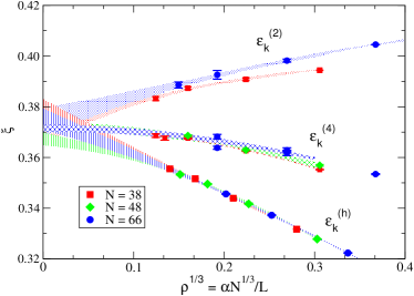
Figure 1: (color online) The calculated ground state energy shown as the value of $\xi$ versus the lattice size for various particle numbers and Hamiltonians.

We have calculated the ground-state energy for different particle numbers and lattice sizes. The time-step errors have been extrapolated to zero within statistical errors, and walker population biases have been checked and were found to be negligible for the population sizes used. The imaginary time step is $\approx 0.01$ - $0.05\ E_{F}^{-1}$ , the total propagation time is of order $10$ - $30\ E_{F}^{-1}$ and 2,000-20,000 random walkers are used in the simulations.

For $N=4$, we found that the use of BCS importance functions reduced the statistical error by a factor of $10$, or $100\times$ reduction in computer time, compared to the usual FG importance function. The improvement increased to $1500\times$ for $N=38$ in a $12^{3}$ lattice. For larger systems, the discrepancy is much larger still; indeed the statistical fluctuations from the latter are such that often meaningful results cannot be obtained with the run configurations described above.

In Fig. 1 we summarize our calculations of the energy as a function of $\rho^{1/3}$ where $\rho=N/N_{k}^{3}$, and the particle number is $N=38$, $48$ or $66$. We plot $\xi$, Eq. 1, where we have in all cases used the infinite system free-gas energy $E_{FG}=\tfrac{3}{5}\tfrac{\hbar^{2}k_{F}^{2}}{2m}$ with $k_{F}^{3}=3\pi^{2}\frac{N}{\alpha N_{k}^{3}}$ as the reference.

Hamiltonian	$N$	$\xi$	err	$A$	err
$\epsilon_{k}^{(2)}$	14	0.39	0.01	0.21	0.12
	38	0.370	0.005	0.14	0.04
	66	0.374	0.005	0.11	0.04
$\epsilon_{k}^{(4)}$	38	0.372	0.002
	48	0.372	0.003
	66	0.372	0.003
$\epsilon_{k}^{(h)}$	4	0.280	0.004	-0.28	0.05
	38	0.380	0.005	-0.17	0.03
	48	0.367	0.005	-0.05	0.03
	66	0.375	0.005	-0.13	0.03

Table 2: Energy extrapolations to infinite volume, zero range limit for various particle numbers $N$ and different Hamiltonians. The term linear in the effective range, $A$, is also shown where it is not tuned to zero.

DMC calculations have found converged results when using 66 particlesForbes:2011 ; Gandolfi:2011 , and our results confirm this. The differences between 38 and 66 particles are rather small. Our calculations with 14 particles show a significant size dependence, and with 26 particles the effects are still noticeable. These are not shown on the figure. We have also computed the energy for 4 particle systems for a variety of lattice sizes and find agreement with Ref. Bour:2011 . The error bands in the figure provide least-squares estimates for the one sigma error based upon quadratic fits to the finite-size effects. The fits are of the form $E/E_{FG}=\xi+A\rho^{1/3}+B\rho^{2/3}$. For the interactions tuned to $r_{e}=0$, a fit with $A$ fixed to zero is used. Including a linear coefficient in the fit yields a value statistically consistent with zero.

The extrapolation in lattice size for the $k^{2}$ and Hubbard dispersions show opposite slope as expected from the opposite signs of their effective ranges. The extrapolation to $\rho\rightarrow 0$ is consistent with $\xi=0.372(0.005)$ in all cases. Our final error contains statistical component and the errors associated with finite population sizes and finite time-step errors. This value is below previous experiments, but more compatible with recent experimental results of the Zwierlein groupZwierlein:2011 .

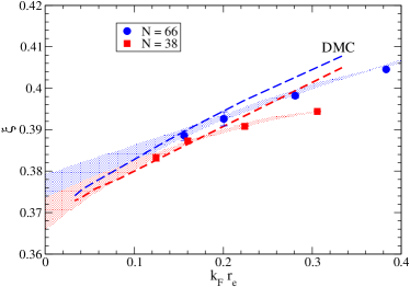
Figure 2: (color online) The ground-state energy as a function of $k_{F}r_{e}$: comparison of DMC and AFQMC results. Dashed lines are DMC results, shifted down by 0.02 to enable comparison of the slopes.

We have also examined the behavior of the energy as a function of $k_{F}r_{e}$ for finite effective ranges. It has been conjecturedWerner:2010 that the slope of $\xi$ is universal: $\xi(r_{e})=\xi+Sk_{F}r_{e}$. Of course a finite range purely attractive interaction is subject to collapse for a many-particle system, but a small repulsive many-body interaction or the lattice, where double occupancy of a single species is not allowed, is enough to stabilize the system. Our results are consistent with the universality conjecture. In particular our results for zero effective range approach the continuum limit with a slope consistent with zero.

Figure 2 compares the AFQMC results for the $\epsilon_{k}^{(2)}$ interaction with the DMC results Forbes:2011 ; Gandolfi:2011 for various values of the effective range. The AFQMC produces somewhat lower energies than the DMC, consistent with the upper-bound nature of the DMC calculations. For the slope $S$ of $\xi$ with respect to finite $r_{e}$, the fit to the $N=66$ AFQMC results yields $S=0.11(.03)$. Similar fits to the AFQMC data with the Hubbard dispersion $\epsilon_{k}^{(h)}$ for $N=66$ yield a linear term of $S=0.12(.03)$. Both are in agreement with the DMC results of $S=0.12(.01)$.Gandolfia:2011

In summary, we have shown how to incorporate a pairing importance function into auxiliary field quantum Monte Carlo algorithms and used it to treat the unitary Fermi Gas. This algorithm, for attractive interactions and equal spin populations, is exact and can be extended to large lattices and strong interactions. We find $\xi=0.372(.005)$ using a variety of interactions tuned to unitarity. We also find a slope of the ground state energy with effective range of S= 0.12 (.03) for the different lattice and continuum Hamiltonians. This method should be useful without modification for the entire BCS/BEC transition and for studying many other properties of cold Fermi gases. It can also be applied to a wide variety of problems in other strongly-correlated fermions, in areas ranging from cold atoms to condensed matter to quantum chemistry to nuclear physics.

- (1) J. Carlson, S.-Y. Chang, V. R. Pandharipande, and K. E. Schmidt, Phys. Rev. Lett. 91, 050401 (2003)
- (2) S. Y. Chang, V. R. Pandharipande, J. Carlson, and K. E. Schmidt, Phys. Rev. A 70, 043602 (2004)
- (3) G. Astrakharchik, J. Boronat, J. Casulleras, and S. Giorgini, Phys. Rev. Lett. 93, 200404 (2004)
- (4) M. Bartenstein, A. Altmeyer, S. Riedl, S. Jochim, C. Chin, J. H. Denschlag, and R. Grimm, Phys. Rev. Lett. 92, 203201 (2004)
- (5) J. Kinast, A. Turlapov, J. E. Thomas, Q. Chen, J. Stajic, and K. Levin, Science 307, 1296 (2005)
- (6) G. B. Partridge, W. Li, R. I. Kamar, Y.-a. Liao, and R. G. Hulet, Science 311, 503 (2006)
- (7) L. Luo and J. E. Thomas, J. Low Temp. Phys. 154, 1 (2009)
- (8) N. Navon, S. Nascimbène, F. Chevy, and C. Salomon, Science 328, 729 (2010)
- (9) M. W. Zwierlein(2011), talk presented at the Fermions from Cold Atoms to Neutron Stars Experimental Symposium, Institute for Nuclear Theory, Seattle, WA, May 16-20 2011
- (10) J. Carlson and S. Reddy, Phys. Rev. Lett. 95, 060401 (2005)
- (11) C. Lobo, I. Carusotto, S. Giorgini, A. Recati, and S. Stringari, Phys. Rev. Lett. 97, 100405 (2006)
- (12) M. M. Forbes, S. Gandolfi, and A. Gezerlis, Phys. Rev. Lett. 106, 235303 (2011)
- (13) S. Gandolfi, K. E. Schmidt, and J. Carlson, Phys. Rev. A 83, 041601 (2011)
- (14) J. Bardeen, L. N. Cooper, and J. R. Schrieffer, Phys. Rev. 108, 1175 (1957)
- (15) J. B. Anderson, J. Chem. Phys. 65, 4121 (1976)
- (16) S. Zhang, J. Carlson, and J. E. Gubernatis, Phys. Rev. Lett. 74, 3652 (1995)
- (17) S. Zhang, J. Carlson, and J. E. Gubernatis, Phys. Rev. B 55, 7464 (1997)
- (18) S. Zhang and H. Krakauer, Phys. Rev. Lett. 90, 136401 (2003)
- (19) C.-C. Chang and S. Zhang, Phys. Rev. Lett. 104, 116402 (2010)
- (20) W. A. Al-Saidi, S. Zhang, and H. Krakauer, J. Chem. Phys. 124, 224101 (2006)
- (21) W. Purwanto, H. Krakauer, and S. Zhang, Phys. Rev. B 80, 214116 (2009)
- (22) D. Lee, Phys. Rev. B 73, 115112 (2006)
- (23) A. Bulgac, J. E. Drut, and P. Magierski, Phys. Rev. Lett. 96, 090404 (2006)
- (24) D. Lee, Phys. Rev. B 75, 134502 (2007)
- (25) D. Lee, Phys. Rev. C 78, 024001 (2008)
- (26) D. Lee, Eur. Phys. J. A 35, 171 (2008)
- (27) S. Bour, X. Li, D. Lee, U.-G. Meissner, and L. Mitas, Phys. Rev. A 83, 063619 (2011)
- (28) W. Ketterle and M. W. Zwierlein, in Ultracold Fermi Gases, edited by M. Inguscio, W. Ketterle, and C. Salomon (IOSPress, Amsterdam, 2008) arXiv:0801.2500v1
- (29) J. E. Hirsch, Phys. Rev. B 28, 4059 (1983)
- (30) F. Werner and Y. Castin(2010), arXiv:1001.0774
- (31) S. Gandolfi(2011), fig. 2 includes updated DMC results at small