Gyrokinetic simulations of the tearing instability

Abstract

Linear gyrokinetic simulations covering the collisional – collisionless transitional regime of the tearing instability are performed. It is shown that the growth rate scaling with collisionality agrees well with that predicted by a two-fluid theory for a low plasma beta case in which ion kinetic dynamics are negligible. Electron wave-particle interactions (Landau damping), finite Larmor radius, and other kinetic effects invalidate the fluid theory in the collisionless regime, in which a general non-polytropic equation of state for pressure (temperature) perturbations should be considered. We also vary the ratio of the background ion to electron temperatures, and show that the scalings expected from existing calculations can be recovered, but only in the limit of very low beta.

I Introduction

The tearing instability Furth et al. (1963) is important in magnetic fusion devices, where it drives the formation of magnetic islands that can significantly degrade heat and particle confinement Waelbroeck (2009). The related micro-tearing mode Drake and Lee (1977) may lead to background turbulence and is also a source of confinement loss. Solar flares and substorms in the Earth’s magnetosphere are some of the many other contexts where tearing plays a crucial role, inducing magnetic reconnection, explosive energy release and large-scale reconfiguration of the magnetic field Biskamp (2000).

The evolution of the tearing instability critically depends on the relationship between the width of the current layer, $\delta$, where the frozen-flux condition breaks down and reconnection takes place, and the length scales characteristic of kinetic or non-magnetohydrodynamic (MHD) effects, such as the ion and electron skin-depths, $d_{\mathrm{i}}=c/\omega_{pi}$ and $d_{\mathrm{e}}=c/\omega_{pe}$, the ion-sound Larmor radius, $\rho_{s}=c_{s}/\Omega_{ci}$, and the ion and electron Larmor radii, $\rho_{\mathrm{i}}$ and $\rho_{\mathrm{e}}$ (see below for precise definitions of these scales; for $T_{e}\sim T_{i}$, $\rho_{s}\sim\rho_{\mathrm{i}}$). For sufficiently large electron-ion collision frequency, $\nu_{e}$, the width of the reconnection layer well-exceeds all of these non-MHD scales and the mode, at least in the limit of strong guide-field and sufficiently low $\beta$, is expected to be well described by well-known resistive MHD theory Furth et al. (1963); Rutherford (1973); Coppi et al. (1976); Waelbroeck (1989); Militello and Porcelli (2004); Escande and Ottaviani (2004); Loureiro et al. (2005). In many plasmas of interest (e.g., the Earth’s magnetosphere, modern large tokamaks), however, this is not the case: a decrease in the collisionality of the plasma leads to a decrease in the resistivity, causing the current layer width to shrink until it reaches or falls below the largest relevant non-MHD scale; in the strong guide-field case of interest here, this scale is typically (for $\beta>m_{e}/m_{i}$) the ion-scale $\lambda_{i}$, where $\lambda_{i}\sim\rho_{s}\sim\sqrt{\beta}d_{i}$ for $\beta\ll 1$ and $\lambda_{i}\sim d_{i}$ for $\beta\sim 1$ and larger. For plasmas in which $T_{0i}/T_{0e}\equiv\tau\gtrsim 1$ ($T_{0i,e}$ are the ion and electron background temperatures), $\delta\lesssim\rho_{\mathrm{i}}$ in this case, suggesting that a kinetic treatment of the ions dynamics is necessary.

Given the complexity of a fully kinetic treatment, a variety of simplified models have been employed to analytically describe tearing in such cases. These range from cold-ion ($e.g.$, Ahedo and Ramos (2009); Fitzpatrick (2010)) or warm-ion ($e.g.$, Loureiro and Hammett (2008); Del Sarto et al. (2011)) two-fluid approximations to calculations that include some sub-set of ion and electron kinetic effects (notably perpendicular ion FLR effects or electron Landau damping)  Drake and Lee (1977); Cowley et al. (1986); Porcelli (1991); Zakharov and Rogers (1992); Zocco and Schekochihin (2011). A further complication of the $\delta\ll\lambda_{i}$ regime, however, is that the tearing mode becomes coupled to pressure perturbations related to electron and/or ion diamagnetic drifts, for example, and most existing analytic calculations deal with this by invoking some type of ad-hoc closure assumption, $e.g$ isothermal or adiabatic electron or ion equations of state. Such closures potentially play an even greater role as $\beta$ approaches or exceeds unity, in which coupling to the sound-waves (slow waves) along the magnetic field is also typically important. Here we find, based on fully gyrokinetic simulations of the linear tearing mode across a range of parameters, that when two-fluid effects become non-negligible ($\delta\lesssim\lambda_{i}$), there is not, in general, a simple relationship between the pressure and density fluctuations for either the ions or electrons. The ratio between the two becomes a complicated function of position that cannot be described by simple closure relations. This poses a serious challenge to theoretical studies of collisionless or weakly collisional reconnection, particularly at higher $\beta\sim 1$ and $T_{e0}\lesssim T_{0i}$ where $\delta\sim\rho_{\mathrm{e}}$, since a rigorous treatment would seem to require fully kinetic treatments of both the perpendicular and parallel electron and ion responses. The gyrokinetic ion and electron model used here allows us to explore numerically, over a range of plasma parameters in the strong guide-field limit of a simple slab geometry, the kinetic physics of the tearing mode and the applicability of some existing theories as the system transitions from the collisional to collisionless regimes.

II Numerical setup

We carry out simulations in doubly-periodic slab geometry using the gyrokinetic code AstroGK Numata et al. (2010). The equilibrium magnetic field profile is

$$\bm{B}=B_{z0}\hat{z}+B_{y}^{\mathrm{eq}}(x)\hat{y},\quad B_{z0}\gg B_{y}^{\mathrm{eq}},$$ (1)

where $B_{z0}$ is the background magnetic guide field and $B_{y}^{\mathrm{eq}}$ is the in-plane, reconnecting component, related to the parallel vector potential by $B_{y}^{\mathrm{eq}}(x)=-\partial A_{\parallel}^{\mathrm{eq}}/\partial x$. From the formal point of view, $B_{y}^{\mathrm{eq}}$ is a first-order gyrokinetic perturbation. To set it up, we perturb the background (Maxwellian) electron distribution function $f_{0\mathrm{e}}(v)$ with a shifted Maxwellian $\delta f_{\mathrm{e}}\propto v_{\parallel}$ ($v$, $v_{\parallel}$ are the velocity-space coordinates), yielding

$$A_{\parallel}^{\mathrm{eq}}(x)=A_{\parallel 0}^{\mathrm{eq}}\cosh^{-2}\left(\frac{x-L_{x}/2}{a}\right)S_{\mathrm{h}}(x),$$ (2)

where $A_{\parallel 0}^{\mathrm{eq}}=3\sqrt{3}/4$ (such that $\max|B_{y}^{\mathrm{eq}}(x)|=1.0$), and $S_{\mathrm{h}}(x)$ is a shape function to enforce periodicity Numata et al. (2010). The equilibrium scale length is denoted by $a$ and $L_{x}$ is the domain length in the $x$-direction, set to $L_{x}/a=3.2\pi$. In the $y$-direction, we set $L_{y}/a=2.5\pi$, resulting in a value of the tearing instability parameter $\Delta^{\prime}a\approx 23.2$ Loureiro et al. (2005) for the longest wavelength mode in the system: $k_{y}a=2\pi a/L_{y}=0.8$. Constant $background$ temperatures ($T_{0\mathrm{i},\mathrm{e}}$) and densities ($n_{0\mathrm{i},\mathrm{e}}$) are assumed for both species. We consider a quasi-neutral plasma, so $n_{0{\mathrm{i}}}=n_{0{\mathrm{e}}}=n_{0}$, and singly charged ions $q_{\mathrm{i}}=-q_{\mathrm{e}}=e$.

We employ a model collision operator which satisfies physical requirements Abel et al. (2008); Barnes et al. (2009) and is able to reproduce Spitzer resistivity Spitzer and Härm (1953), for which the electron-ion collision frequency ($\nu_{\mathrm{e}}$) and the resistivity ($\eta$) are related by

$$\eta/\mu_{0}=0.380\nu_{\mathrm{e}}d_{\mathrm{e}}^{2}$$ (3)

with $\mu_{0}$ being the vacuum permeability; this formula holds for $k_{\perp}d_{\mathrm{e}}\lesssim 1$ ($k_{\perp}^{-1}$ is a characteristic scale length perpendicular to a mean magnetic field, $k_{\perp}^{-1}\sim\delta$ for the tearing instability). Like-particle collisions are neglected.

AstroGK employs a pseudo-spectral algorithm to discretize the GK equation in the spatial coordinates $(x,y)$. For the linear runs reported here, it is sufficient to keep only one harmonic in the $y$-direction (the lowest harmonic is the fastest growing one). The number of Fourier modes in the $x$-direction ranges from $512$ to $8192$ (multiplied by $2/3$ for dealising). Velocity space integrals are evaluated using Gaussian quadrature; the velocity grid is fixed to $20\times 16$ collocation points in the pitch-angle and energy directions, respectively. Convergence tests have been performed in all runs to confirm the accuracy of our results.

III Problem setup

We scan in collisionality and use Eq. (3) to calculate the plasma resistivity $\eta$, recast in terms of the Lundquist number, $S=\mu_{0}aV_{\mathrm{A}}/\eta=2.63(\nu_{\mathrm{e}}\tau_{\mathrm{A}})^{-1}(d_{\mathrm{e}}/a)^{-2}$, where $V_{\mathrm{A}}$ is the Alfvén velocity corresponding to the peak value of $B_{y}^{\mathrm{eq}}$ and $\tau_{\mathrm{A}}\equiv a/V_{\mathrm{A}}$ is the Alfvén time. Other relevant quantities are:

$$\begin{split}\rho_{\mathrm{i}}=\tau^{1/2}\rho_{\mathrm{Se}}\sqrt{2},~{}~{}~{}&d_{\mathrm{i}}=\beta_{\mathrm{e}}^{-1/2}\rho_{\mathrm{Se}}\sqrt{2},\\ \rho_{\mathrm{e}}=\sigma^{1/2}\rho_{\mathrm{Se}}\sqrt{2},~{}~{}~{}&d_{\mathrm{e}}=\beta_{\mathrm{e}}^{-1/2}\sigma^{1/2}\rho_{\mathrm{Se}}\sqrt{2},\end{split}$$ (4)

where $\rho_{i,e}$ and $d_{i,e}$ are the ion and electron Larmor radii and skin-depths, respectively, $\sigma\equiv m_{\mathrm{e}}/m_{\mathrm{i}}$, $\tau\equiv T_{0\mathrm{i}}/T_{0\mathrm{e}}$, $\beta_{\mathrm{e}}\equiv n_{0}T_{0\mathrm{e}}/(B_{z0}^{2}/2\mu_{0})$, $\rho_{\mathrm{Se}}\equiv c_{\mathrm{Se}}/\Omega_{\mathrm{ci}}$, $c_{\mathrm{Se}}=\sqrt{T_{0\mathrm{e}}/m_{\mathrm{i}}}$, $\Omega_{\mathrm{ci}}=eB_{z0}/m_{\rm i}$, $\rho_{s}=\rho_{\mathrm{Se}}\sqrt{(}1+\tau)$. In addition to $\nu_{\mathrm{e}}$, the adjustable parameters considered here include the mass ratio $\sigma$, the electron beta $\beta_{\mathrm{e}}$, $\rho_{\mathrm{Se}}/a$, and $\tau$, although the latter is held fixed at $\tau=1$ except where stated otherwise.

We study the collisional–collisionless transition by scanning in collisionality. As $\nu_{e}$ is decreased, the different ion and electron kinetic scales become important. Given the challenge of clearly separating all the relevant spatial scales in a kinetic simulation, we split our study into two sets of runs: a smaller-$\rho_{\mathrm{Se}}$ series ($\rho_{\mathrm{Se}}/a=0.02/\sqrt{2}\simeq 0.014$) and a larger-$\rho_{\mathrm{Se}}$ series ($\rho_{\mathrm{Se}}/a=0.2/\sqrt{2}\simeq 0.14$). Since $\tau=1$ is held fixed except at the end of the article, these two sets of runs also typically correspond to $\rho_{\mathrm{i}}/a=0.02$ and $\rho_{\mathrm{i}}/a=0.2$, respectively.

In the former set $\rho_{e},~{}d_{e}\ll\lambda_{\mathrm{i}}\lesssim\delta\ll a$; in this case the frozen-flux condition is broken by collisions alone, and since $\delta$ well exceeds the collisionless electron scales $\rho_{e},~{}d_{e}$, such scales need not be resolved in the simulations. The ion response, on the other hand, is predominantly collisional ($\delta>\lambda_{i}$) at the smallest considered values of $S\sim 500$ but kinetic ($\delta\lesssim\lambda_{i}$) at the largest values, $S\sim 10^{5}$. Thus resistive MHD would be expected, at least marginally, to be valid in this case at the smaller $S$ values. In the set of runs with larger-$\rho_{\mathrm{Se}}$ ($\rho_{\mathrm{Se}}/a\simeq 0.14$), we again consider $\rho_{e},~{}d_{\mathrm{e}}\ll\lambda_{\mathrm{i}}\lesssim a$, but since $\rho_{\mathrm{Se}}/a$ is ten times larger than in the previous set of runs, the ions in this second set are predominantly kinetic ($\delta\lesssim\lambda_{i}$) over the entire considered range of $S\sim 100-10^{6}$. Indeed, at the highest values of $S$, $\delta$ reaches collisionless electron scales ($d_{e}$ at $\beta\ll 1$ and $\rho_{e}$ at $\beta\sim 1$), and the instability dynamics become essentially collisionless.

In both sets of runs, we vary $S$ over the ranges mentioned above for three different sets of $\beta_{\mathrm{e}}$ and $\sigma=m_{e}/m_{i}$: [($\beta_{\mathrm{e}}$, $\sigma$)=(0.3,0.01), (0.075,0.0025), (0.01875,0.000625)]. These parameters are such that $\rho_{\mathrm{Se}}/d_{e}\equiv\sqrt{\beta_{e}/(2\sigma)}=\sqrt{15}\simeq 3.9$ is held fixed and thus, since $\rho_{s}/a$ is also held fixed (at either 0.014 or 0.14), $d_{e}/a$ is also held fixed (at either 0.0037 or 0.037, respectively). Given the parameter dependences of $d_{i}$ and $\rho_{e}$ noted in Eq. 4, however, it is seen that the values of $d_{i}/a$ and $\rho_{e}/a$ both change as $\beta_{e}$ and $\sigma$ are varied in this manner: for $\rho_{\mathrm{Se}}=0.014$, $d_{i}=0.02/\sqrt{\beta_{e}}$ and $\rho_{e}/a=0.02\sqrt{\sigma}$, while for $\rho_{\mathrm{Se}}/a=0.14$ they are ten times larger.

IV Smaller $\rho_{\mathrm{Se}}/a=0.014$

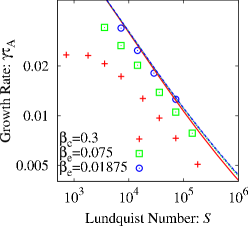
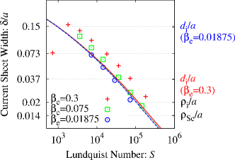
Figure 1: (Color online) Growth rate and current sheet width versus the Lundquist number for $\rho_{\mathrm{Se}}/a=0.02/\sqrt{2}$. Red crosses, green squares, and blue circles show gyrokinetic results for $(\beta_{\mathrm{e}},\sigma)=(0.3,0.01),(0.075,0.0025),(0.01875,0.000625)$, respectively. Red solid, green dashed and blue dot-dashed lines are the corresponding two-fluid Fitzpatrick (2010) scalings. The relevant scale lengths are identified on the right axis of the right panel.

Fig. 1 shows the tearing mode growth rate ($\gamma\tau_{A}=d\log A_{\parallel}/dx$ evaluated at the $X$-point) and current layer width (full-width at half-maximum - typically somewhat larger than the current-profile scale-length, depending on the current profile) as functions of the Lundquist number (symbols) for $T_{i0}=T_{e0}$. Also plotted (lines) are the results obtained from a reduced two fluid model Fitzpatrick (2010) with an isothermal electron equation of state. This model is derived under the assumption of low-$\beta$, but exactly how low $\beta$ must be for the validity of this model depends on how the various quantities in the model are ordered and is thus problem-dependent. For the ordering assumed in Fitzpatrick (2010), it is argued that $\beta_{e}\ll\sqrt{\sigma}$ is required — a condition that is marginally satisfied here only for the lowest $\beta$ case, $(\beta_{\mathrm{e}},\sigma)=(0.01875,0.000625)$. The two fluid model is also derived under the assumption of cold ions, but as we show later (see fig. 4), the difference between the gyrokinetic results at $\tau=0$ and $\tau=1$ is small.

For the largest value of the collisionality, $S\lesssim 10^{3}$, the gyrokinetic growth rates roll-over because the current layer width is too wide to satisfy the asymptotic scale separation, $\delta\ll a$, assumed in the two-fluid model tearing mode dispersion relation that is plotted in the figure. The deviation between the gyrokinetic and two-fluid results at the lowest $S$ values should therefore be disregarded. It is seen from the right panel that, as noted earlier, $\delta>\lambda_{i}$ for all but the largest $S$ values (recall that $\lambda_{i}$, the outer-most collisionless ion-scale of relevance, is typically $\lambda_{i}\sim\rho_{\mathrm{Se}}\sim\rho_{\mathrm{i}}\ll d_{i}$ for $\beta\ll 1$ and $\lambda_{i}\sim\rho_{\mathrm{Se}}\sim d_{i}$ for $\beta_{e}=0.3$). In this case, as expected, the two-fluid model, at least at low-$\beta$, recovers the well-known single-fluid resistive-MHD scalingsFurth et al. (1963) and is thus independent of $\beta_{\mathrm{e}}$. Defining the dimensionless parameter $C_{k}=k_{y}a^{2}B^{\prime}(0)/B_{0}$ where $B^{\prime}(0)$ is the derivative of the equilibrium reconnecting field at the X-point, $k_{y}$ is the linear mode-number, and $B_{0}$ is the normalizing field (for our parameters $k_{y}a=0.8$ and and $aB^{\prime}(0)/B_{0}=2.6$ so that $C_{k}=2.08$ for all runs), the general one-fluid scalings are most compactly written in terms of the quantities $\tau_{Ak}=a/(V_{A}C_{k})=\tau_{A}/C_{k}$ and $S_{k}=C_{k}S$. Two scalings are obtained depending on the product of $\Delta^{\prime}\delta$; defining $C_{\Delta}=\Delta^{\prime}a/2$ (equal to 11.6 in our runs), they are

$$\gamma\tau_{Ak}\simeq S_{k}^{-1/3}\ ,~{}\delta/a\sim S_{k}^{-1/3}\text{ for }\Delta^{\prime}\delta/2\gg 1,$$ (5)

$$\gamma\tau_{Ak}\simeq 0.96S_{k}^{-3/5}C_{\Delta}^{4/5}\ ,~{}\delta/a\sim S_{k}^{-2/5}C_{\Delta}^{1/5},$$

$$\qquad\qquad\qquad\qquad\qquad\qquad\qquad\text{ for }\Delta^{\prime}\delta/2\ll 1.$$ (6)

For the parameters of our simulations ($C_{k}=2.08$ and $C_{\Delta}=11.6$) these can also be written in terms of $\tau_{A}$ and $S$ as

$$\gamma\tau_{A}\simeq 1.63S^{-1/3}\ ,~{}\delta/a\sim 0.78S^{-1/3}\text{ for }\Delta^{\prime}\delta/2\gg 1,$$ (7)

$$\gamma\tau_{A}\simeq 9.14S^{-3/5}\ ,~{}\delta/a\sim 1.22S^{-2/5}\text{ for }\Delta^{\prime}\delta/2\ll 1.$$ (8)

The small and large $\Delta^{\prime}$ expressions for $\gamma$ and $\delta/a$ both break-down at the point of maximum growth rate, where they are roughly equal: $S_{k}\sim C_{\Delta}^{3}$, or for our parameters, $S\sim 600$. Since $S$ is larger or comparable to this value in the simulations presented here, most of our runs are in the either the marginally-large or small-$\Delta^{\prime}$ regimes. Using for example the small-$\Delta^{\prime}$ expressions for the value $S=10,000$, we obtain $\delta/a\simeq 0.03$ and $\gamma\tau_{A}\simeq 0.04$, in rough agreement with the numerical results. The over-estimation of the growth rates by the two fluid model at higher $\beta_{e}\sim 0.3$ is possibly due to either a breakdown in the low-$\beta$ ordering of the fluid model or a gradual onset of kinetic effects ($e.g.$ the invalidity of a simple isothermal equation of state, as discussed further below).

V Larger $\rho_{\mathrm{Se}}/a=0.14$

We set $\rho_{\mathrm{Se}}/a=0.2/\sqrt{2}=0.14$ and adjust $\nu_{\mathrm{e}}$ such that $\delta\lesssim\lambda_{\mathrm{i}}$, thus focusing on the regime where ion kinetic effects are important. The growth rate and current layer width versus the Lundquist number are shown in Figure 2 (the label $S=\infty$ identifies the case $\nu_{\mathrm{e}}=0$; we note that $S$ may be underestimated if $\delta\lesssim d_{\mathrm{e}}$ since Eq. (3) is not valid in such a regime). These runs correspond to the same set of ($\beta_{\mathrm{e}}$, $\sigma$) as before; in terms of length scales, $d_{\mathrm{e}}/a\approx 0.037$ is fixed, and $d_{\mathrm{i}}$ and $\rho_{\mathrm{e}}$ change.

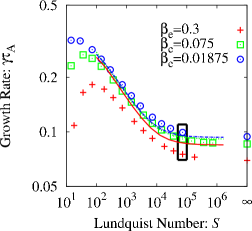
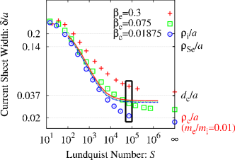
Figure 2: (Color online) Growth rate and current sheet width versus the Lundquist number for $\rho_{\mathrm{Se}}/a=0.2/\sqrt{2}$. Color and symbol schemes are the same as in Fig. 1. The scale lengths labelled on the right panel are fixed except $\rho_{\mathrm{e}}$ (only $\rho_{\mathrm{e}}$ for $\sigma=0.01$ is shown). The points in the box are used to diagnose temperature fluctuations in Fig. 3.

As in the previous case, we observe better agreement between the GK and two fluid results for lower values of $\beta_{\mathrm{e}}$; however, as $S$ increases and the collisionless regime is approached, the agreement becomes poorer for any value of $\beta_{\mathrm{e}}$. In this regime, electron kinetic effects (Landau damping and even finite electron orbits: note that for $\beta_{\mathrm{e}}=0.3$, $\delta/\rho_{\mathrm{e}}\approx 2$) play an important role; these are absent in the two fluid model.

VI Temperature fluctuations

To better understand the discrepancies between the GK and two fluid results (at high-$\beta_{\mathrm{e}}$ regardless of the collisionality and at any $\beta_{\mathrm{e}}$ in the collisionless regime), we examine in Fig. 3 the validity of the isothermal closure by diagnosing the temperature fluctuations for the $\rho_{\mathrm{Se}}/a=0.2/\sqrt{2}$ and $S\approx 7.2\times 10^{4}$ case. In Fig. 3, we plot the eigenfunctions of the temperature, density and electrostatic potential ($\phi$), and the diagonal components of the pressure tensor fluctuations normalized by $\tilde{n}$. These are measures of the polytropic indices $\Gamma_{s}$ because, according to the polytropic law, $\tilde{p}_{s}=\Gamma_{s}T_{0s}\tilde{n}_{s}$ ($s=\mathrm{i},\mathrm{e}$ is a species label). We define $\Gamma_{\perp,s}=(\Gamma_{xx,s}+\Gamma_{yy,s})/2$ and $\Gamma_{\parallel,s}=\Gamma_{zz,s}$, but restrict the discussion to the parallel temperature for electrons as the perpendicular component is at least marginally smaller (by a factor of ${\mathcal{O}}[(k_{\perp}\rho_{\mathrm{e}})^{2}]$) in Ohm’s law.

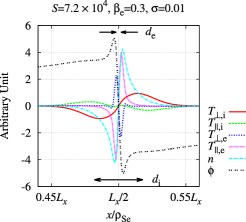
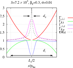
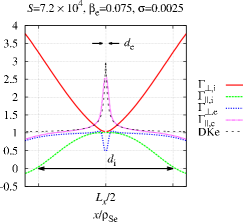
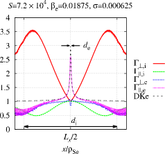
Figure 3: (Color online) Eigenfunctions for the $\beta_{\mathrm{e}}=0.3$ case, and the polytropic indices of ions and electrons in the perpendicular and the parallel directions. A spatially changing polytropic index means the equation of state is not polytropic.

As seen in the figure, while $\Gamma_{\parallel,\mathrm{e}}\sim 1$ outside the layer (thus validating the isothermal electron approximation in that region), it is highly peaked in the current layer ($x\sim d_{\mathrm{e}}$) due to the Landau damping. A spatially varying polytropic index means that the equation of state is not polytropic, and thus the isothermal closure is violated. Also plotted is $\Gamma_{\parallel,\mathrm{e}}$ obtained analytically from the drift-kinetic electron (DKe) model Drake and Lee (1977). We observe that this expression provides an excellent fit to our data for the case $\beta_{\mathrm{e}}=0.01875$, where electron FLR effects are negligible. As for the ions, $\Gamma_{\mathrm{i}}$ also varies widely over the ion inertial scale in all cases, again invalidating simple equations of state for this species.

VII Ion background temperature

Finally, we examine the effect of the ion background temperature ($\tau$), as this is the other possible source of discrepancy between the GK and the two fluid results.

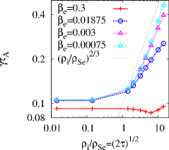
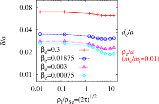
Figure 4: (Color online) Ion temperature dependence of the tearing growth rate and current layer width.

Plotted in Figure 4 are the growth rate and current layer width versus $\rho_{\mathrm{i}}/\rho_{\mathrm{Se}}$. As before, we probe different values of $\beta_{\mathrm{e}}$ and change $\sigma$ such that $\rho_{\mathrm{Se}}/a\approx 0.14$, $d_{\mathrm{e}}/a\approx 0.037$ in all cases. The Lundquist number is $S\approx 7200$. As in Ref. Rogers et al. (2007), we find that the growth rate is remarkably insensitive to $\tau$ for large $\beta_{\mathrm{e}}$; however, as $\beta_{e}$ decreases we are able to recover the theoretically predicted scaling Porcelli (1991) of $\gamma\tau_{A}\sim\tau^{1/3}$. One possible explanation of these results is that, at higher $\beta_{e}$, coupling to sound-waves becomes more important and even more strongly invalidates the simple closure relations used in the fluid calculations.

VIII Discussion and Conclusions

We have performed a set of gyrokinetic simulations of the linear tearing instability, varying the collisionality, plasma $\beta$, mass ratio $m_{e}/m_{i}$, and $T_{i}/T_{e}$. Although we find agreement with a two-fluid description Fitzpatrick (2010) in the collisional low-$\beta$ case, one of our main conclusions is that if the plasma parameters are such that two fluid effects are important, there is not, in general, a simple relationship between the pressure and density fluctuations, their ratio being a function of position. This is an intrinsically kinetic effect which cannot be captured by any known fluid closure. It seems likely that in our simulations, at non-small values of $\beta$, the parallel sound wave dynamics become important and ion flow and temperature must be solved for kinetically. In addition, we find that electron Landau damping cannot be neglected in the collisionless regime. If $\delta>\rho_{\mathrm{e}}$, the effects of finite electron orbits can be neglected, and the Landau damping effect is analytically tractable using the drift-kinetic model (DKe) Drake and Lee (1977). For $\delta\sim\rho_{\mathrm{e}}$ the DKe model is not sufficient and a fully kinetic treatment is required.

We have also shown that for $\beta_{\mathrm{e}}\ll 1$ (such that the ion sound wave and the Alfvén wave are decoupled), the theoretically predicted dependence of the growth rate on $\tau$, $\gamma\sim\tau^{1/3}$ Porcelli (1991) is verified. However, for $\beta_{\mathrm{e}}\sim 1$ the growth rate in our system is remarkably insensitive to the background ion temperature, as noted in previous numerical studies  Rogers et al. (2007).

As is widely known, linear theory breaks down when the magnetic island width grows beyond the width of the current layer, and indeed, in some physical systems, turbulent noise seems likely to generate seed magnetic islands that are nonlinear from birth. It is therefore important to understand the importance of kinetic effects in the nonlinear phase — a topic not studied here. The answer to this, particularly in the strong guide-field limit in which 3D kinetic simulations are only just starting to be explored, will likely depend on the aspect of reconnection that is of interest. As in the case of relatively small systems without a guide field, it may be that gross features of the reconnection, such as the reconnection rate, can be, at least qualitatively, captured by fluid models. On the other hand, in weakly collisional plasmas, as suggested by the results found here, it seems likely that questions involving particle heating or energy partition, for example, will likely require a kinetic physics model that includes effects such as Landau damping and goes beyond simple closure schemes. The potential strength of the gyrokinetic model — and weakness, in some physical problems — is that it is designed to study the strong guide-field limit, in which time-resolution of the electron gyroperiod (necessary in particle simulations, for example, but not in gyrokinetics) can become a formidable challenge. Further work is needed to explore nonlinear reconnection in the strong guide-field limit, and understand the contributions that gyrokinetic simulations may offer.

IX Acknowledgments

The authors thank M. Furukawa, F. Jenko, V. V. Mirnov, M. Püschel, J. J. Ramos, Z. Yoshida, and A. Zocco for useful comments, and A.A. Schekochihin for numerous suggestions that much improved this manuscript. This work was supported by the DOE Center for Multiscale Plasma Dynamics, the DOE-Espcor grant to CICART, the Leverhulme Trust Network for Magnetized Turbulence, the Wolfgang Pauli Institute (Vienna, Austria) Fundação para a Ciência e a Tecnologia (Portugal) and the European Community under the contract of Association between EURATOM and IST. The views and opinions expressed herein do not necessarily reflect those of the European Commission. Simulations were performed on TACC, NICS, NCCS and NERSC supercomputers.

References

- Furth et al. (1963) H. P. Furth, J. Killeen, and M. N. Rosenbluth, Phys. Fluids 6, 459 (1963).
- Waelbroeck (2009) F. L. Waelbroeck, Nucl. Fusion 49, 104025 (2009).
- Drake and Lee (1977) J. F. Drake and Y. C. Lee, Phys. Fluids 20, 1341 (1977).
- Biskamp (2000) D. Biskamp, Magnetic Reconnection in Plasmas (Cambridge Univ. Press, Cambridge, 2000), ISBN 0-521-58288-1.
- Rutherford (1973) P. Rutherford, Phys. Fluids 16, 1903 (1973).
- Coppi et al. (1976) B. Coppi, R. Pellat, M. Rosenbluth, P. Rutherford, and R. Galvão, Sov. J. Plasma Phys. 2, 533 (1976).
- Waelbroeck (1989) F. Waelbroeck, Phys. Fluids B 1, 2372 (1989).
- Militello and Porcelli (2004) F. Militello and F. Porcelli, Phys. Plasmas 11, L13 (2004).
- Escande and Ottaviani (2004) D. Escande and M. Ottaviani, Phys. Lett. A 323, 278 (2004).
- Loureiro et al. (2005) N. F. Loureiro, S. C. Cowley, W. Dorland, M. G. Haines, and A. A. Schekochihin, Phys. Rev. Lett. 95, 235003 (2005).
- Ahedo and Ramos (2009) E. Ahedo and J. J. Ramos, Plasma Phys. Control. Fusion 51, 055018 (2009).
- Fitzpatrick (2010) R. Fitzpatrick, Phys. Plasmas 17, 042101 (2010).
- Loureiro and Hammett (2008) N. F. Loureiro and G. W. Hammett, J. Comp. Phys. 227, 4518 (2008).
- Del Sarto et al. (2011) D. Del Sarto, C. Marchetto, F. Pegoraro, and F. Califano, Plasma Phys. Control. Fusion 53, 035008 (2011).
- Cowley et al. (1986) S. Cowley, R. M. Kulsrud, and T. S. Hahm, Phys. Fluids B 29, 3230 (1986).
- Porcelli (1991) F. Porcelli, Phys. Rev. Lett. 66, 425 (1991).
- Zakharov and Rogers (1992) L. Zakharov and B. Rogers, Phys. Fluids B 4, 3285 (1992).
- Zocco and Schekochihin (2011) A. Zocco and A. A. Schekochihin, arXiv:1104.4622 (2011).
- Numata et al. (2010) R. Numata, G. G. Howes, T. Tatsuno, M. Barnes, and W. Dorland, J. Comput. Phys. 229, 9347 (2010).
- Abel et al. (2008) I. G. Abel, M. Barnes, S. C. Cowley, W. Dorland, and A. A. Schekochihin, Phys. Plasmas 15, 122509 (2008).
- Barnes et al. (2009) M. Barnes, I. G. Abel, W. Dorland, D. R. Ernst, G. W. Hammett, P. Ricci, B. N. Rogers, A. A. Schekochihin, and T. Tatsuno, Phys. Plasmas 16, 072107 (2009).
- Spitzer and Härm (1953) L. Spitzer, Jr. and R. Härm, Phys. Rev. 89, 977 (1953).
- Rogers et al. (2007) B. N. Rogers, S. Kobayashi, P. Ricci, W. Dorland, J. Drake, and T. Tatsuno, Phys. Plasmas 14, 092110 (2007).