The Spitzer ice legacy: Ice evolution from cores to protostars

Abstract

Ices regulate much of the chemistry during star formation and account for up to 80% of the available oxygen and carbon. In this paper, we use the Spitzer $c2d$ ice survey, complimented with data sets on ices in cloud cores and high-mass protostars, to determine standard ice abundances and to present a coherent picture of the evolution of ices during low- and high-mass star formation. The median ice composition H₂O:CO:CO₂:CH₃OH:NH₃:CH₄:XCN is 100:29:29:3:5:5:0.3 and 100:13:13:4:5:2:0.6 toward low- and high-mass protostars, respectively, and 100:31:38:4:–:–:– in cloud cores. In the low-mass sample, the ice abundances with respect to H₂O of CH₄, NH₃, and the component of CO₂ mixed with H₂O typically vary by $<$25%, indicative of co-formation with H₂O. In contrast, some CO and CO₂ ice components, XCN and CH₃OH vary by factors 2–10 between the lower and upper quartile. The XCN band correlates with CO, consistent with its OCN^- identification. The origin(s) of the different levels of ice abundance variations are constrained by comparing ice inventories toward different types of protostars and background stars, through ice mapping, analysis of cloud-to-cloud variations, and ice (anti-)correlations. Based on the analysis, the first ice formation phase is driven by hydrogenation of atoms, which results in a H₂O-dominated ice. At later prestellar times, CO freezes out and variations in CO freeze-out levels and the subsequent CO-based chemistry can explain most of the observed ice abundance variations. The last important ice evolution stage is thermal and UV processing around protostars, resulting in CO desorption, ice segregation and formation of complex organic molecules. The distribution of cometary ice abundances are consistent with with the idea that most cometary ices have a protostellar origin.

1 Introduction

Star formation begins with the collapse of an interstellar cloud core to form a protostar, which grows from infall of envelope material and later through an accretion disk, where planets may form. This physical evolution from cores to planetary systems is accompanied by a chemical evolution, which will affect planet and planetesimal compositions. Much of this chemical evolution takes place in icy mantles on interstellar grain surfaces, and the aim of this paper is to consolidate the knowledge of ice evolution during star formation coming out of the Spitzer Space Telescope mission.

The first ices were detected in the interstellar medium almost 40 years ago (Gillett & Forrest, 1973) and from previous work, mostly toward high-mass protostars, H₂O, CO and CO₂ ices are known to be common during the cold and dense stages of star formation, with abundances reaching 10^-4 $n_{\rm H_{2}}$. The ice mantles also contain smaller amounts of CH₃OH, CH₄, NH₃ and XCN (e.g Gibb et al., 2004). CH₃OH and other ices are proposed sources of complex organic molecules (Charnley et al., 1992; Garrod et al., 2008; Öberg et al., 2009b) and determining ice abundances and production channels in star forming regions is therefore of great interest for studies of prebiotic chemistry. Most ices except for CO are predicted to form in situ on interstellar grain surfaces through hydrogenation and oxygenation of atoms and small molecules (Tielens & Hagen, 1982). Heat and UV radiation from protostars may result in additional ice processing and Gibb et al. (2004) suggested that some CO₂ ice, and all CH₃OH and XCN ice form through such processing based on observations toward high-mass protostars with the Infrared Space Observatory (ISO). This has been challenged by observations of abundant CH₃OH and XCN ice toward low-mass protostars (Pontoppidan et al., 2003b; van Broekhuizen et al., 2005), where ices are protected from strong UV fields during most of their life time.

Spitzer’s high sensitivity made it possible to observe ices toward low mass protostars and background stars at 5–30 $\mu$m. The $c2d$ program (Evans et al., 2003) obtained IRS spectra of 50 low-mass protostars (Boogert et al., 2008; Pontoppidan et al., 2008; Öberg et al., 2008; Bottinelli et al., 2010, from now on Paper I-IV), providing an unprecedented sample size that complements the ISO data on high-mass protostars. Additional Spitzer ice observations exist on ices toward background sources, looking through molecular clouds at a range of extinctions (Bergin et al., 2005; Knez et al., 2005; Pontoppidan, 2006; Whittet et al., 2009; Boogert et al., 2011) and toward protostars in a high-UV environment (Reach et al., 2009).

Because the Spitzer spectrometer had a lower cutoff at $\lambda\sim 5$ $\mu$m, complete ice inventories can only be obtained by adding complementary ground-based spectroscopy to cover the strong 3 $\mu$m H₂O, the 4.65 $\mu$m CO, the 4.6 $\mu$m XCN, and the 3.53 $\mu$m CH₃OH features. The latter feature has been used to validate the use of the 9.7 $\mu$m feature to derive CH₃OH ice abundances (Paper I). The XCN feature has been shown empirically to consist of two components, whose relative contributions to the feature vary from source to source (van Broekhuizen et al., 2005). One of the components can be securely assigned to OCN^- from comparison with laboratory spectra, while the carrier of the second component, peaking at 2175 cm^-1, is unknown. Suggested carriers of the 2175 cm^-1 component include OCN^- present in a different ice environment, resulting in a different spectrum, as well as completely different molecules (Pendleton et al., 1999; van Broekhuizen et al., 2004).

In the analysis of astrophysical ice spectra, comparison with laboratory ice spectra is key, both to identify ice species (such as OCN^- above) and to characterize the ice morphology; i.e., some ice bands, such as CO and CO₂, cannot be fitted by a single laboratory ice mixture, but seem to trace molecules in two or more ice phases (Tielens et al., 1991; Chiar et al., 1995; Dartois et al., 1999, Paper II). Traditionally the observed spectra have been directly compared to a superposition of pure and mixed ice spectra, characterizing the ice morphology in each source independently (e.g. Merrill et al., 1976; Gibb et al., 2004; Zasowski et al., 2009). The constraints are often degenerate, however, since ice spectral features vary with ice composition, temperature and radiation processing. To address this, ice bands have instead been decomposed phenomenologically into a small set of unique spectral components (e.g. Tielens et al., 1991; Pendleton et al., 1999; Keane et al., 2001; Pontoppidan et al., 2003a, and §2.2). The contributions of the derived components are then used to characterize the spectral bands in all sources in the sample. This method was employed in papers I and II. Because all observed spectra are decomposed into the same, small number of components this method provides information on the sample as a whole, i.e. it directly shows which parts of the spectral profile are ubiquitous and which are environment dependent. This is crucial information when assigning a component carrier – without this, the degeneracy is almost always too large to draw conclusions about the structure of the ice from spectral profiles alone.

Building on the analysis in Paper I-IV, this paper aims to establish an ice evolution scenario that also takes into account the present knowledge of ice abundances toward cloud cores (Boogert et al., 2011) and high-mass protostars (Gibb et al., 2004). Section 2 summarizes the sample characteristics. Section 3 presents new ice data for 10 low-mass protostars, followed by ice abundance medians toward low- and high mass protostars. The variation among the low-mass protostellar abundances are investigated followed by comparison of this ice sample with ices toward high-mass protostars, low-mass protostars in a high-radiation environment, and background stars. The reasons for the abundance variations seen for some ice features are further explored through analysis of spatial differences and correlation studies. Further, new data are used to test previous hypotheses about the carrier(s) of the XCN band. The results are discussed in §4 with respect to different ice formation scenarios and ice chemistry in low-mass versus high-mass star-forming regions.

2 Sample and ice features

2.1 Sample

Spitzer-IRS spectra were obtained for $\sim$50 low-mass protostars with ice features as part of the $c2d$ Legacy program (PIDs 172 and 179), a dedicated open time program (PID 20604) and a Guaranteed Time Observations (GTO) program (PI Houck). All sources were included in Papers II-III on CO₂ and CH₄, while the $c2d$ sources alone were investigated in Paper I and IV.

The Spitzer spectra were complemented by ground-based Keck/NIRSPEC (McLean et al., 1998) and VLT/ISAAC (Moorwood, 1997) L-band spectra of the H₂O ice 3 $\mu$m feature. In addition, the combined sample partly overlaps with a 3–5 $\mu$m VLT survey of CO and XCN ice toward low-mass protostars (Pontoppidan et al., 2003b; van Broekhuizen et al., 2005) and additional CO observations were obtained with Keck/NIRSPEC (Paper II). The VLT survey contains many sources in Ophiuchus, for which the Spitzer data are taken from GTO programs. These sources are key for a comprehensive investigation of how the XCN complex, composed of OCN^- and potentially a second carrier, relates to other ices. The reduction of the spectra to obtain abundances are described in the individual c2d papers and the additional GTO sources have been reduced using an identical procedure to those presented in Papers I and IV.

The low-mass sample is complemented with 9 ISO sources, representative of high-mass protostars, from Gibb et al. (2004) which were re-analyzed in Papers I-III to ensure that the low- and high-mass ice abundances are consistently derived using the same component analysis and band strengths. The sources were not included in Paper IV, and NH₃ abundances are therefore taken from Gibb et al. (2004). In summary, our sample consists of 63 YSOs, that have been analyzed in a homogenous way. When compared with ice abundances toward background stars from Knez et al. (2005) and Boogert et al. (2011), this sample spans all evolutionary stages from molecular clouds to disks and six orders of magnitude in stellar luminosities and a range of star-forming environments.

2.2 Ice features

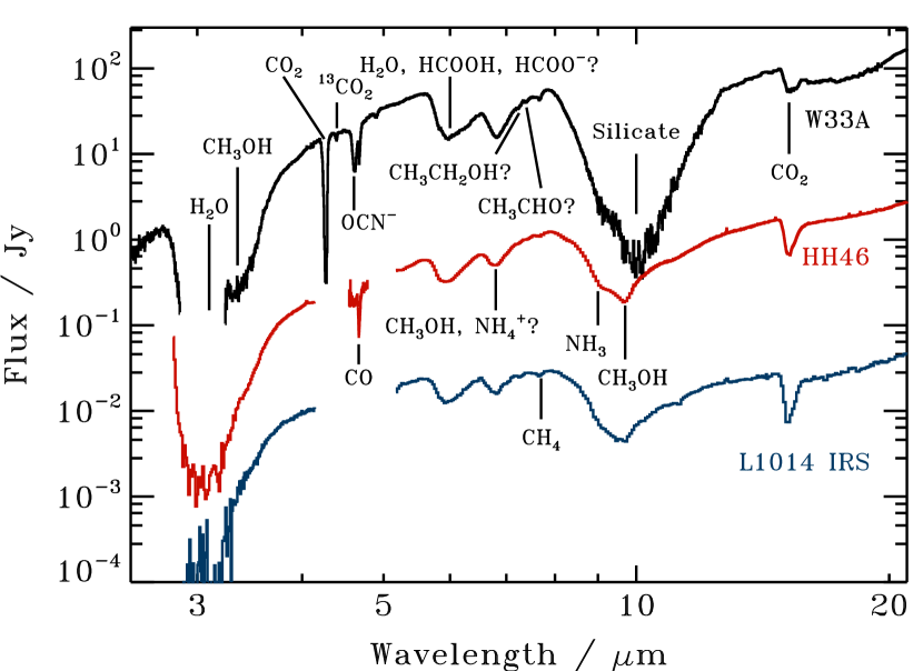
Figure 1: Ice spectra toward the protostars W33A (10⁵ L_⊙), HH46 (12 L_⊙) and L1014 IRS (0.09 L_⊙) (Gibb et al., 2000; Boogert et al., 2004, Paper I). The 3 $\mu$m portions of the spectra have been binned to increase the S/N.

Figure 1 shows the main ice features seen toward background stars and protostars with the identifications of different bands to H₂O, CO, CO₂, CH₃OH, NH₃, CH₄ and OCN^- ice marked. H₂O column densities are derived from the 3 $\mu$m band whenever such data are available; otherwise the librational band (10–30 $\mu$m) is used. CH₃OH and NH₃ abundances are generally derived from the 9–10 $\mu$m bands. OCN^- abundances are derived from one of the two components (centered at 2165 cm^-1) that together make up the XCN band (the total band centered at 4.62 $\mu$m next to the CO feature). The OCN^- identification is based on laboratory spectra. The abundance of the second XCN carrier (associated with the ‘2175 cm^-1’ band) is derived assuming the OCN^- band strength.

The CO and CO₂ spectral features can be decomposed into a number of components corresponding to CO and CO₂ in different ice mixtures (Pontoppidan et al., 2003b, Paper II). CO is decomposed into three components corresponding to pure CO ice, CO mixed with CO₂ (CO:CO₂) and CO mixed with H₂O ice (CO:H₂O). CO₂ is similarly decomposed into four components corresponding to pure CO₂ ice, CO₂ mixed with CO (CO₂:CO), CO₂ mixed with H₂O ice (CO₂:H₂O) and a shoulder which has been associated with CO₂ mixed with CH₃OH (Dartois et al., 1999).

More tentative identifications of spectral bands to HCOOH, NH${}_{4}^{+}$, CH₃CH₂OH and CH₃CHO are also marked in Fig. 1. Most of these tentative identifications are found in a complex band between 5 and 7 $\mu$m. To constrain the carriers of this band it was decomposed into five different components (C1–C5) after subtraction of the contribution from H₂O ice in Paper I. C1 and C2 make up the 6 $\mu$m band, C3 and C4 the 6.8 $\mu$m band and C5 is a broad, underlying feature that covers the entire 5–7 $\mu$m region. From comparison with laboratory ice spectra, C1 has been identified with HCOOH and H₂CO, C2 with HCOO^- and NH₃, C3 with NH${}_{4}^{+}$ and CH₃OH, C4 with NH${}_{4}^{+}$ and C5 with warm H₂O and anions (Paper I).

3 Results

Figure 1 shows the similar 3–20 $\mu$m spectra toward protostars spanning orders of magnitude in luminosities, suggestive of a partly shared ice formation history during all types of star formation. The spectra are not identical, however, and median abundances of identified ices toward low- and high-mass protostars are presented in §3.2. Ice abundance variations toward low-mass protostars are further investigated in §3.3 to constrain which ice form together with H₂O and which do not. In §3.4 the low-mass sample is contrasted with ice abundance distributions toward high-mass protostars to test the significance of any differences noted in §3.2. §3.5 continues with a comparison of ice distributions between clouds and protostars to constrain which ices require protostellar processing to form. §3.6. presents an analysis of spatial variations in ice abundances, both on large-scale between clouds, and on small scales within a single core. Finally, ice correlations are used in §3.7 to provide further constraints on XCN formation, and H₂O ice anti-correlations are presented to investigate which ices form in competition with H₂O.

3.1 New ice abundances in Ophiuchus

To enlarge the sample of low-mass sources with available XCN data, a set of GTO data in Ophiuchus was analyzed in the same way as the $c2d$ sources. The five components, C1–5, from Paper I are fitted to the 5–7 $\mu$m complex with their peak optical depths as free parameters. The NH₃ and CH₃OH abundances toward the same sources are determined from their 9.0 and 9.7 $\mu$m features, using a 4^th order polynomial to remove the underlying silicate feature (Paper IV). After continuum subtraction, column densities are derived by fitting two Gaussians to the observed spectra around the expected band positions and using the same band strengths as in Paper IV (Table 1). The flux and optical depth spectra are shown in Appendix A together with fitted peak positions and band widths. While NH${}_{4}^{+}$ is not explicitly discussed here except in the context of the N-budget, maximum abundances for the Ophiuchus sources can be extracted from Table 1 using the same conversion factor as in Paper I. HCOOH abundances are not reported, since the previously used feature may have a significant contribution from other carriers (Appendix B). The presence of a feature at 7.25 $\mu$m is in itself evidence for the formation of complex ices, even though its dominating carrier (probably HCOOH or CH₃CH₂OH) is speculative.

3.2 Median abundances

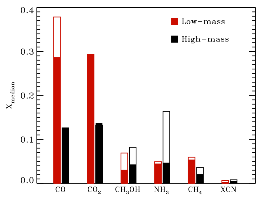
Figure 2: Median abundances with respect to H₂O in the low- and high-mass protostellar samples (X_median) derived using survival analysis that includes upper limits (filled bars) and median detected abundances (outlined bars) toward low- and high-mass protostars.

Figure 2 shows the median ice abundances with respect to H₂O ice for low- and high-mass protostars, calculated from Paper I-IV and from the new Ophiuchus values reported in Table 1. All ice abundances are expressed with respect to H₂O because H₂O ice forms early during star formation, is the most abundant ice, and has a high sublimation point. The median values are calculated: 1) using only the detections, and 2) using the Kaplan-Meier (KM) estimate of the survival function. The latter is a non-parametric procedure that takes into account the constraints provided by upper limits. When calculating the KM estimate the detections and upper limits are ordered from low to high and the upper limits are given the values of the nearest lower detections. For example in a sample of four detections of 0.5, 1, 3 and 4 and an upper limit of $<$2, the upper limit is treated as a detection of 1. The KM estimate and how to apply statistical tests on it is reviewed by Feigelson & Nelson (1985). The medians calculated from the KM estimate provide more accurate descriptions of ice populations with significant upper limits as demonstrated in Fig. 2, where the low- and high-mass CH₃OH medians and the NH₃ and CH₄ median toward high-mass protostars are 40-70% lower when taking into account the upper limits.

Table 2 lists the medians that best describe the data set for total ice abundances, while Table 3 provides medians for all ice components together with their lower and upper quartile values. Quartiles are favored over standard deviations since most ice abundances do not follow a normal distribution (see below). For the species where the Kaplan-Meier estimate is $>$20% lower than the detection-based median, both are listed. CO and CO₂ are the most abundant ices after H₂O, with low-mass protostellar median abundances of 29% with respect to H₂O. NH₃, CH₃OH and CH₄ have comparable median abundances of 3-5%, while XCN is rare at $<$1%. The CH₃OH and NH₃ abundance medians are similar toward low- and high-mass protostars, when the upper limits toward high-mass protostars are taken into account, while CO, CO₂ and CH₄ are more abundant and XCN is less abundant toward low-mass protostars. The low CO₂ abundances in this high-mass sample are consistent with recent observations of CO₂ ice abundances of 10–18% toward high-mass protostars in the galactic center, but not toward high-mass YSOs in the LMC (An et al., 2009; Oliveira et al., 2011). Testing whether perceived differences between low- and high-mass protostars are significant requires an investigation of the ice abundance distributions within each sample of protostars, however, and this is done in §3.4 after presenting ice abundance variations toward low-mass protostars in §3.3.

3.3 Ice abundance variations

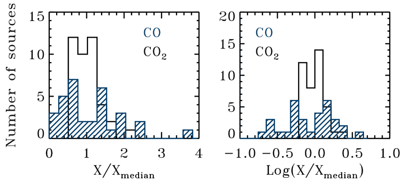
Figure 3: Histograms of the CO (blue line-filled) and CO₂ (black contours) abundances toward low-mass protostars with respect to the median abundances. The left panel shows the skewed abundance distributions of both molecules and the right panel the more symmetric log-normalized histograms.

Ice abundance variations between different sources depend on how sensitive the ice formation and destruction pathways are to the local environment. Investigating protostellar abundance variations thus puts constraints on when and where different ices form (variations are not dominated by reported abundance uncertainties from fitting the observed spectra). Figure 3 demonstrates that some ice abundance distributions are skewed with a high-abundance tail. All abundance histograms are therefore log-transformed and then centered on the median detected low-mass protostellar ice abundance, with bin sizes proportional to the low-mass abundance variances. For ices where the median is unaffected or barely affected ($<$20%) by including upper limits, the detections alone are shown. For ice abundances that are better constrained by including upper limits (CO, CH₃OH, XCN, OCN^-, 2175 cm^-1, C2 and C5 toward low-mass protostars and CH₃OH, NH₃, CH₄, XCN, CO:CO₂ and C5 toward high-mass protostars), the distributions include 3-$\sigma$ upper limits. Appendix C contains figures that compare the distributions with and without upper limits included. Differences between low- and high-mass protostellar abundances are discussed further below, while this section focuses on the larger low-mass sample.

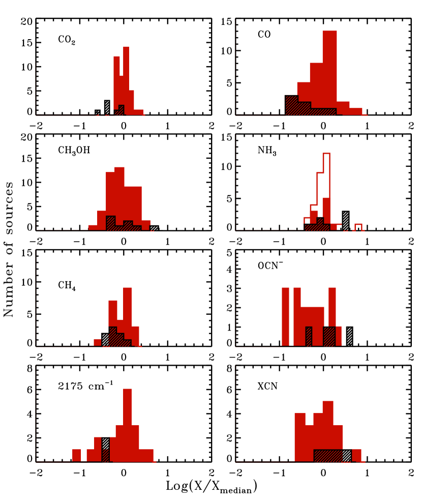
Figure 4: Histograms of total ice abundances toward low-mass protostars (red) and high-mass protostars (black). For low-mass NH₃ abundances, the solid filled histograms are from Paper IV using a silicate template to extract NH₃ and the contoured histograms are from Paper IV and Table 1 when using a polynomial to fit the local continuum around the NH₃ feature.

Since ice abundances are with respect to H₂O, a small variation of a species indicates co-formation with H₂O, while large ice abundance variations are indicative of different formation and/or destruction dependencies than H₂O ice. Figure 4 shows that the total CO₂, CH₄ and NH₃ abundance distributions are narrow, while CO, OCN^-, the 2175 cm^-1 XCN component and CH₃OH have broader distributions with order of magnitude abundance variations between different sources. Figure 5 shows that the narrow CO₂ distribution is due to CO₂:H₂O ice, while all other CO₂ and CO component distributions are broad. The pure CO and CO₂ ice components have the broadest distributions, consistent with their expected dependence on the protostellar envelope temperature for ice evaporation and segregation. The 5–7 $\mu$m components, C1–5, span the full range of variations observed among the identified ice components, including the previously noted narrow C3 distribution (Paper I).

Protostellar ice heating was explored in Paper I and II as explanations for observed abundance variations, using pure CO/CO:H₂O and pure CO₂/CO₂:H₂O as diagnostics of the amount of moderate ice heating, and H₂O/silicate as a probe of complete ice sublimation. Correlations between H₂O/silicate and the different C1-5 components are extensively discussed in Paper I and by Boogert et al. (2011) for protostars and background stars. The main conclusion was that C3/C4 does depend on ice sublimation, supporting its identification with low- and high-temperature NH${}_{4}^{+}$ salts.

Moderate ice heating is predicted to reduce the abundances of volatile ices (decreasing the pure CO abundance), segregate previous ice mixtures (resulting in pure CO₂), drive ice crystallization, activate acid-base chemistry and cause diffusion of ice radicals and thus the formation of more complex species. None of the ice abundances in this study are however correlated with either ice temperature tracer (not shown) except for the previously found C5/H₂O correlation with pure CO/CO:H₂O (Paper I). Moderate (transient) ice heating alone seems to play a minor role in simple ice formation. This result does not exclude that the combined differences in temperature and UV radiation around low- and high-mass protostars results in different ice chemistries. Whether this is the case is the topic of next section.

3.4 Low- versus high-mass protostars

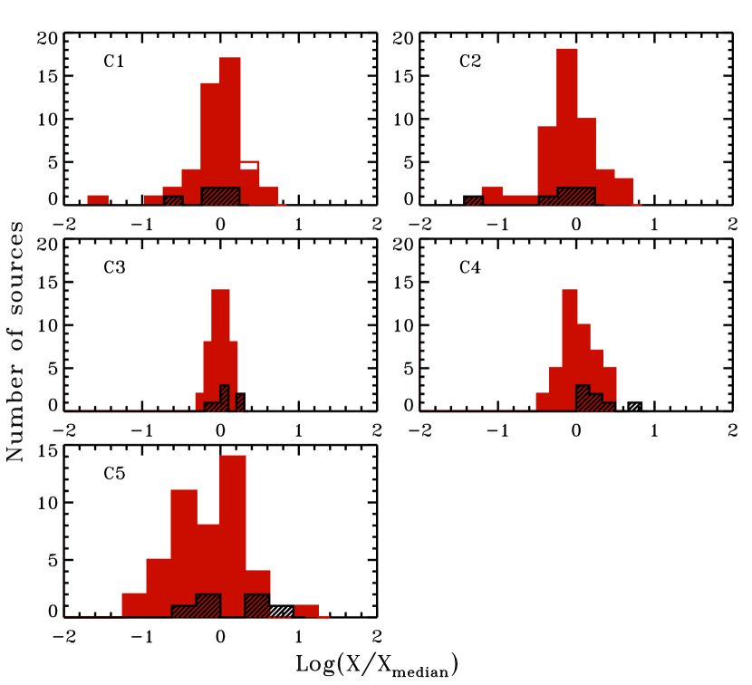
Figure 6: Histograms of 5-7 $\mu$m components, otherwise as in Fig. 4.

Figures 4–6 show that many ices are similarly distributed toward low- and high-mass protostars, but as noted in §3.2, the total CO₂, CO and CH₄ abundances are lower toward the high-mass sources. Figure 5 reveals that the difference in CO₂ abundances between low-mass and high-mass stars is due to a difference in the CO₂:H₂O ice component, which typically dominate the spectra toward low-mass sources (Paper II). All CO components are centered around a lower value toward high-mass protostars compared to low-mass protostars. Among the C1–5 components, C4 seems more abundant toward high-mass protostars.

The significance of the visual differences in Figs. 2,4–6 and other proposed differences between low-mass and high-mass protostars can be evaluated statistically. Kruskal-Wallis one-way analysis of variance by ranks is a non-parametric method to test the equality of medians in two or more groups of observations (Kruskal & Wallis, 1952). The test statistic does not assume normal distributions and is given by

$$K=(N-1)\frac{\Sigma^{g}_{i=1}n_{i}(\bar{r}_{i}-\bar{r})^{2}}{\Sigma^{g}_{i=1}\Sigma_{j=1}^{n_{i}}(\bar{r}_{ij}-\bar{r})^{2}},$$ (1)

where $g$ is the number of groups, $n_{i}$ is the number of observations (ice abundances) in group $i$ (low or high-mass protostars), $r_{ij}$ is the rank of observation $j$ in group $i$ (here the rank of a source in terms of the investigated ice abundance), $N$ is the total number of observations across all groups, $\bar{r}_{i}$ is the mean rank of group $i$ and $\bar{r}$ is the mean rank in the whole population. The null hypothesis of equal medians is rejected when $K\geq\chi^{2}_{\alpha:g-1}$ where $\alpha$ is the significance level and $g-1$ the degrees of freedom for the $\chi^{2}$ statistic. The $\chi^{2}_{\alpha:g-1}$ values can be looked up in tables and are also part of most statistic packages such as $R$.

Applying the test to the low-mass versus high-mass detected ice abundances shows that there is a significant difference (at the 95% level) between the two samples for CO₂, CO, CO₂:H₂O, pure CO and C4 ice abundances. Differences in C5, CH₃OH or OCN^-, which have been suggested to be more efficiently formed toward high-mass protostars, are not statistically significant. To check whether including upper limits affect these results, a similar test (the logrank test) was run in $R$ using the previously calculated Keplar-Meier estimates and the function survdiff. The results are consistent with the Kruskal-Wallis test, except that CH₄ is different in low -and high-mass stars at the 98% confidence level when including upper limits.

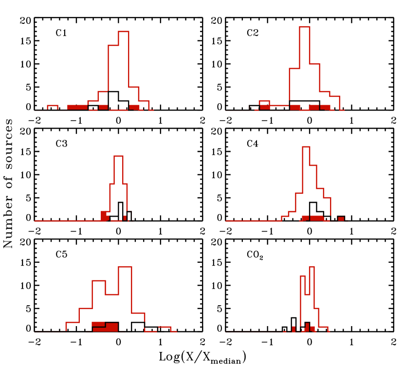
Figure 7: Histograms of CO₂ and the C1-C5 components (including upper limits) toward low-mass protostars (red contours), high-mass protostars (black contours) and the four IC 1396A sources (red solid).

In the above analysis, all low-mass protostars are situated in star-forming regions without any nearby massive stars. It is therefore difficult to disentangle which differences are intrinsic to the low- versus high-mass star-forming processes and which differences depend on the local radiation environment. IC 1396A, known as the Elephant Trunk Nebula, is a dense globule, excited by the 4 Myr old O6 star HD 206267. Ice observations – H₂O, CO₂ and C1-5 – toward four low-mass protostars are presented by Reach et al. (2009). The C3/C4 ratio toward these protostars resembled the ratio found toward high-mass protostars, suggesting that the ice evolution around low-mass protostars depends on the external radiation environment. Figure 7 shows a histogram comparison for the CO₂ and C1-5 abundances toward the low-mass, high-mass and IC 1396A samples. Visually the IC 1396A C3 and C4 abundances seem to better overlap with the high-mass sample, while the IC 1396A C5 upper limits and CO₂ detections are more consistent with the low-mass sample. None of these differences are, however, significant, nor is the difference in C3/C4 ratio, likely due to the small IC 1396A sample size.

3.5 Protostars versus background stars

Comparisons between protostars and background stars provide direct limits on which species form before the protostar turns on and starts to heat and irradiate its surroundings. Tables 2 and 3 lists the medians of species detected toward background stars in Serpens and in individual cores (Knez et al., 2005; Boogert et al., 2011). For the isolated core sample we only use those targets with well known H₂O column densities from 3 $\mu$m observations. The upper limits on CH₄, NH₃ and OCN^- are generally too high to be useful and there are only a handful of CO ice observations. C1-5, CO₂ and CH₃OH are, however, detected in a larger number of sources and can be used to compare cloud and protostellar ices.

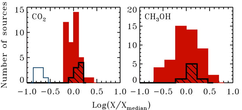
Figure 8: Histograms of CO₂ and CH₃OH toward low-mass protostars (red fill), our background star sample (black line-fill) and Taurus background stars (blue contours).

Previous ice studies toward Taurus revealed a lower CO₂ ice fraction in clouds compared to in low-mass protostellar envelopes (Whittet et al., 2007, Paper II) which together with laboratory studies have encouraged hypotheses of CO₂ formation from energetic processing of CO ice around protostars (e.g., Ioppolo et al., 2009). Similarly, CH₃OH ice has been proposed to be a product of protostellar UV ice-processing (Gibb et al., 2004). Figure 8, using data from Boogert et al. (2011), shows that there is no evidence for different CO₂ and CH₃OH ice abundances toward protostars and background stars. Applying the Kruski-Wallis and Keplar-Meier based tests confirm this lack of a difference in ice composition between our protostellar and cloud sources. Figure 8 also shows the clear difference between Taurus CO₂ ice abundances from Whittet et al. (2007) and our background star ice sample. From this difference, ice abundances toward Taurus background stars are not good templates for ice abundances toward average cloud cores.

In summary, observable ices, except for pure CO₂ ice and the C5 component, are present at the same abundances in the pre-stellar and protostellar phase. Most protostellar ice abundance variations reported in §3.3 must then be due to differences between clouds and to different pre-stellar ice formation processes, rather than thermal and UV processing by the protostar.

3.6 Spatial differences within the low-mass protostellar sample

3.6.1 Cloud-to-cloud variations

Variations in ice formation and destruction efficiencies in the pre-stellar stage may be associated with different cloud structures and initial chemical conditions in different star-forming regions. This is investigated by dividing the low-mass protostellar sample into six groups with sources belonging to the star forming associations in Ophiuchus, Serpens, Corona Australis, Perseus, Taurus and a collection of smaller associations. Kruskal-Wallis tests show that when considered as a whole, the ice abundance medians are statistically indistinguishable between these groups. This is consistent with a Principal Component Analysis in Öberg (2009), which revealed no differences between the different clouds when simultaneously considering all ice abundances.

Cloud-to-cloud variations can also be tested for specific ice components. CO₂ ice abundances in clouds were shown above to be unusually low toward Taurus, while too few CO measurements toward background sources outside of Taurus exist to determine whether CO is lower than expected as well. Testing the CO and CO₂ protostellar differences between the clouds may reveal whether prestellar differences are carried over into the protostellar phase. CH₃OH is another ice that has been observed to be spatially variable (Pontoppidan et al., 2004; Boogert et al., 2011). Differences in the pure CO ice component and the CO₂ shoulder (often assigned to CO₂:CH₃OH interactions) between the clouds are indeed statistically significant at a $>$98% confidence level, while all other CO and CO₂ components and CH₃OH are not. The significant differences exist between the low abundances toward Taurus and the smaller associations on one hand, and the more ’normal’ abundances toward the other clouds (Table 4).

The difference between Taurus and the other clouds is important since much of the current ice paradigm is based on analysis of Taurus sources (e.g. Whittet et al., 2007). The low pure CO ice abundances may also explain the low CH₃OH ice upper limits toward Taurus, since CO freeze-out is a pre-requisite for CH₃OH ice formation without energetic radiation (Cuppen et al., 2009) and a low pure CO ice abundance may indicate that catastrophic CO freeze-out has not taken place. In summary, some CO ice abundance differences seem to be explained by large-scale differences in cloud environments, but overall most cloud and pre-stellar ice formation variability must be due to more local effects than cloud-to-cloud variation. Both from cloud and protostellar ice abundances, Taurus stands out and care should hence be taken in using Taurus trends as a basis for general conclusions on ice evolution during low-mass star formation.

3.6.2 An ice map toward the Oph-F core

Within single cloud cores, ice maps may reveal production and destruction pathways that depend on the local environment. An ice map of protostars in the Oph-F core has been used previously to show that the total CO and the CO:H₂O abundances decrease monotonically away from the central core (Pontoppidan, 2006). The lines of sight probe primarily the dense quiescent core, rather than ice in the protostellar envelopes, and the spatial trends were interpreted as catastrophic freeze-out of CO in the pre-stellar stage once a certain density and temperature is reached. Figure 9 shows that the order of magnitude increase in CO ice with respect to H₂O toward the core is accompanied by an increase in CO₂:CO. In contrast, the CO₂:H₂O ice component is almost constant across the core. The XCN band (the 2175 cm^-1 feature – OCN^- is not detected) is the only other species that increases monotonically toward the densest part of Oph-F. CO₂:CO and the 2175 cm^-1 band thus appear directly related to CO freeze-out. No trend with distance to the core center is seen for any other ice component and is also not expected for ices forming early during cloud formation (e.g. CH₄ and NH₃), which are independent of cloud core time scales and CO freeze-out, or of species dependent on protostellar heating (e.g. pure CO₂ ice) or of components with potentially multiple carriers, such as the C1-5 bands. CH₃OH is only detected toward one of the sources and no trend can thus be extracted. Still the Oph-F map suggests that CO freeze-out followed by a CO driven ice chemistry may account for large pre-stellar ice variations.

3.7 Protostellar correlation studies

The trends found for the Oph-F core are here explored for the entire protostellar sample through correlation studies between especially CO-chemistry products and H₂O ice column densities, and between XCN, and CO and CO₂ ice components.

3.7.1 Dependencies on H₂O ice column

In individual cores, the H₂O column density has been shown to correlate well with dust extinction, assumed to trace the total dust mass and H₂ column (Whittet et al., 1988; Pontoppidan et al., 2004). This implies that the average abundance of H₂O ice per dust grain is constant across the core. In an arbitrary line of sight, the total H₂O ice column density depends on both the column density of dust grains and on the average number of monolayers of H₂O ice on each dust grain. If variations in the H₂O column density across the sample are dominated by the line of sight fraction of high-density material, ices dependent on CO freeze-out are expected to correlate with H₂O column density, since CO freezes out catastrophically at high densities (§3.6.2). If instead variations in the H₂O column density across the sample is dominated by the H₂O abundance on each grain, the main observable trend should be that ices that form in competition with H₂O anti-correlate with the H₂O column density.

In theory, the dust column density can be estimated from the optical depth of the 9.7 $\mu$m silicate feature or from the continuum extinction. Because of a number of practical complications we do not attempt to normalize the H₂O column density to the dust column, however. First, toward protostars, the silicate absorption can be filled in by an unknown amount of silicate emission from the warmer parts of the envelope. Second, continuum extinction estimates are affected by uncertainties in the intrinsic protostellar SEDs. Third, while the 9.7 $\mu$m band correlates well with the near-infrared color excess, the relations vary in different environments by factors of 2 (Chiar et al., 2007; Boogert et al., 2011), possibly because of variations in the grain size distribution or even variations in the grain composition (van Breemen et al., 2011). And fifth, the contribution of unrelated, ice-less foreground dust is often unknown.

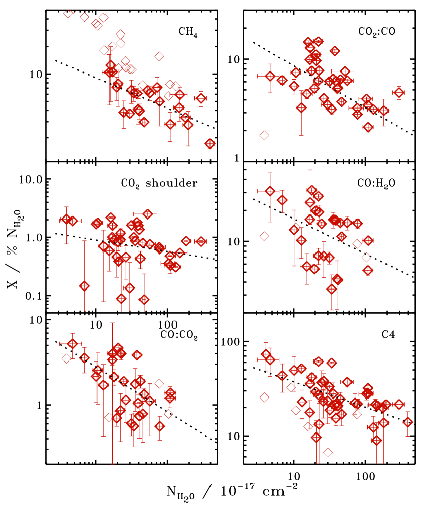
Figure 10: Statistically significant correlations between ice abundances w. r. t. H₂O and the H₂O ice column density for low-mass protostars, with upper limits plotted with thin symbols. The significance of the correlations was measured using Spearman’s rank correlation test, which makes no assumptions about the type of correlation, while the dotted line shows the best log-log fit to the data to guide the eye.

There are no significant positive correlations (at the 95% confidence level) between H₂O and any ice abundance, X/H₂O, when applying Spearman’s rank correlation test (Spearman, 1904) to the low-mass protostellar sample; rank correlation tests are more robust to outliers compared to most parametric correlation tests and make no assumptions about whether the correlation is linear or non-linear. Figure 10 shows that instead, six ice components – CH₄, CO₂:CO, the CO₂ shoulder, CO:H₂O, CO:CO₂ and C4 – are inversely correlated with the H₂O column density at the 97–99% confidence level. C4 has been associated with NH${}_{4}^{+}$ salts and its anti-correlation with H₂O may be explained by an increasing salt fraction with ice sublimation because salts have higher sublimation temperatures than H₂O ice (Paper I). This scenario cannot, however, explain the other anti-correlations, since CH₄, CO and CO₂ are all more volatile than H₂O.

The CO-related anti-correlations may be a result of competitive formation of H₂O and CO; the more oxygen that is bound up in H₂O ice, the less may be available to form gaseous CO and thus ices that depend on CO freeze-out. Still in each individual core CO ice abundances and H₂O ice column densities are expected to correlate because of increasing CO freeze-out toward the densest part of the cloud core. The latter may explain some of the scatter in the plots. Finally, the CH₄–H₂O trend is mainly visible for very low H₂O column densities (many in Ophiuchus) and this relation may be due to more efficient CH₄ formation during only the earliest H₂O formation stage when a large fraction of carbon is still in atomic form.

3.7.2 XCN correlations

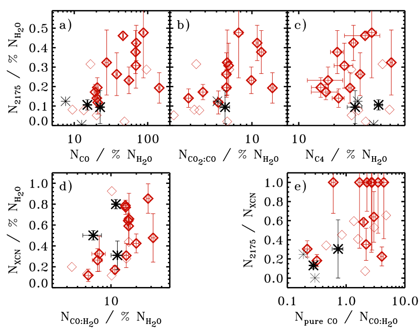
Figure 11: Panels a–d show correlations between XCN and CO ice components for low-mass protostars (red diamonds) with high-mass protstellar abundances shown for comparison (black stars). Panel e shows the relationship between and ice heating tracer and the two XCN components. Thin symbols denote upper limits.

As stated in §1, the XCN band is composed of two components, peaking at 2165 cm^-1 (OCN^-) and at 2175 cm^-1. Toward the Oph-F core, the 2175 cm^-1 component is spatially correlated with CO, CO₂:CO and CO:H₂O. These correlations were explored in the whole low-mass sample and Fig. 11 shows that the 2175 cm^-1 component is significantly correlated with CO and CO₂:CO (95% confidence with Spearman’s rank correlation test) and the correlation is even stronger ($>$99%) when the high-mass sources are added. The complete XCN band is not correlated with either of these components, but it is significantly correlated with the less volatile CO:H₂O component (95% level). Panel e, finally confirms previous claims in van Broekhuizen et al. (2004) that the relative importance of the OCN^- feature and the 2175 cm^-1 feature depend on ice processing, measured here by the pure CO / CO:H₂O ice ratio.

These correlations are indicative of a CO-related, single carrier of the entire XCN band with a spectral profile that depends on the environment. The simplest explanation is that OCN^- is responsible for the entire XCN band (i.e. both the ’OCN^- component’ and the 2175 cm^-1 component) and that the two components are due to OCN^- in a volatile (CO-rich) ice toward some sources, and in a different ice mixture in warm environments. OCN^- can form at 15 K from HNCO in the presence of strong bases (Raunier et al., 2003; van Broekhuizen et al., 2004). Consistent with the 2175 cm^-1 identification with OCN^-, this component seems to be correlated (95% level) with C4 (one of the two bands ascribed to the base NH${}_{4}^{+}$ in Paper I) when only considering low-mass protostellar detections. The correlation is not significant, however, when including the high-mass sample or the significant upper limits and must therefore be considered as tentative.

4 Discussion

4.1 C-, O-, and N-budget

The amount of C, O and N that are typically bound up in ice mantles is important for the life cycle of the elements in the interstellar medium. The total (refractory + volatile) C, O and N abundances in the solar neighborhood are 2.1, 5.8 and 0.58$\times 10^{-4}$ per hydrogen nucleus, respectively (Przybilla et al., 2008). The fractional C, O and N abundance in ices with respect to these total C, N and O abundances are calculated from the presented ice abundances with respect to H₂O ice together with literature values of the H₂O abundance with respect to hydrogen. Pontoppidan et al. (2004) and Boogert & Ehrenfreund (2004) modeled the H₂O abundance toward four of the low-mass protostars in the sample and found $n_{\rm H_{2}O}=4.9\pm 0.7\times 10^{-5}n_{\rm H}$. Toward high-mass protostars the H₂O abundance can be estimated using the relations A${}_{\rm V}/\tau_{\rm 9.7}=9$ and N${}_{\rm H}/A_{\rm V}\sim 1.9\times 10^{21}$ cm^-2 mag^-1 (Roche & Aitken, 1985; Bohlin et al., 1978). It is important to note that this method only provides a crude estimate since the silicate feature is affected both by emission and grain growth; a recent grain model result in a conversion factor that is 30% lower for dense clouds (Evans et al., 2009). Using the values in Gibb et al. (2004) for W33A, NGC7538 IRS 9, Mon R2 IRS 3 and S140 IRS 1 (covering the range of observed ice processing) results in a H₂O abundance of $(5.0\pm 1.9)\times 10^{-5}n_{\rm H}$. A mean H₂O abundance of $5\times 10^{-5}n_{\rm H}$ (i.e. 10^-4 n${}_{\rm H_{2}}$) is therefore assumed for both low and high-mass protostars.

The O abundance in the ice is calculated from $(x_{\rm H_{2}O}+x_{\rm CO}+2\times x_{\rm CO_{2}}+x_{\rm CH_{3}OH}+x_{\rm XCN})\times n_{\rm H_{2}O}$, the C abundance from $(x_{\rm CO}+x_{\rm CO_{2}}+x_{\rm CH_{3}OH}+x_{\rm CH_{4}}+x_{\rm XCN})\times n_{\rm H_{2}O}$ and the N abundance from $(x_{\rm NH_{3}}+x_{\rm XCN}+x_{\rm NH_{4}^{+}})\times n_{\rm H_{2}O}$, where $x_{y}$ is the abundance of $y$ with respect to H₂O. The median upper limit on NH${}_{4}^{+}$ is calculated from the total optical depth of the C3 and C4 components, using the FWHM of 0.195 and 0.292 $\mu$m, respectively from Paper I and a band strength of $4.4\times 10^{-17}$ cm from Schutte & Khanna (2003).

The median percentages of C, O and N bound up in ices, calculated from the ice abundances in Table 2, are listed in Table 5. On average 15% of the total (refractory + volatile) C, 16% of the O and 10% of the N reside in ices toward low-mass protostars. Toward high-mass protostars the same calculation yields 12% of the O, 8% of the C and up to 12% of the N atoms. The differences in the amount of C and O are due to the low CO and CO₂ abundances toward high-mass protostars.

Table 5 also lists the amount of volatile or non-refractory amounts of C and O that are in ices. In the solar neighborhood the non-refractory O abundance is $3.2\times 10^{-4}$ per N_H (Meyer et al., 1998) because a large fraction of O is bound up in silicates and is therefore not available for ice formation (e.g Whittet, 2010). Out of this available O, 34% is bound up in ices toward low-mass protostars, and 25% toward high-mass stars. The fraction of C in refractory material is less well constrained, but assuming a non-refractory C abundance of $\sim 1\times 10^{-4}$ (Weingartner & Draine, 2001) results in 27% of the available C found in ices toward low-mass protostars and 14% toward high-mass protostars.

The above numbers all relate to the median ice abundances in the sample. The extreme ice sources may, however, provide more information on whether ice formation is limited by the elemental abundances. IRS 51 and NGC 7538 IRS 9 are calculated to be the most ice-rich sources in the sample, when still assuming a H₂O ice abundance of $5\times 10^{-5}$ with respect to $n_{\rm H}$. Especially in the case of IRS 51, the amount of O and C found in the ices approaches the abundances of non-refractory O and C (Table 5).

It is important to note that additional O and N may be hidden in the ice in the form of O₂ and N₂. Direct constraints on O₂ ice abundances are high, 50–100% with respect to CO ice, and constraints from O₂ interactions with CO ice are of a similar order (Ehrenfreund et al., 1992; Vandenbussche et al., 1999; Pontoppidan et al., 2003b). O₂ ice is, however, unlikely to be abundant from the low upper limits on O₂ in the gas-phase; it is orders of magnitude less abundant than CO and since the two molecules have similar freeze-out and desorption properties it is unlikely that O₂ is differently partitioned between ice and gas compared to CO (Goldsmith et al., 2000; Pagani et al., 2003; Fuchs et al., 2006).

4.2 Ice evolution: early and late pre-stellar ice formation

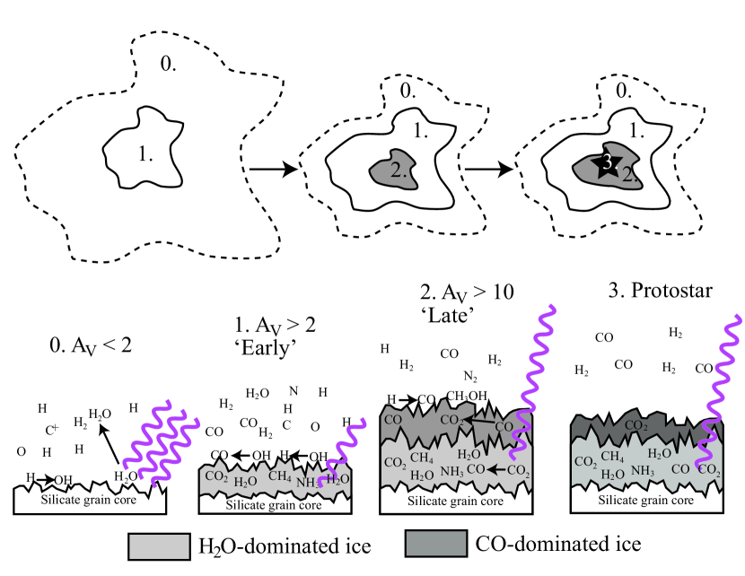
Figure 12: The key ice reactions during the different stages of cloud and star formation, where 0. corresponds to cloud edges where UV photons can penetrate, 1. the early stages of dense cloud formation, 2. the later formation of cloud cores and 3. the protostellar envelope. Ice formation begins in 1. with hydrogenation of atoms resulting in a H₂O dominated ice with a high CO₂ concentration (CO₂:H₂O). At later times CO freezes out catastrophically, resulting in a second layer where CO₂ formation continues (CO₂:CO and CO:CO₂) and CH₃OH formation begins. During all cold stages small amounts of ice chemistry products are maintained in gas-phase due to non-thermal desorption. In the protostellar stage desorption of CO starts at 20 K and H₂O:CO₂ segregation at 30 K.

Toward low- and high-mass protostars alike, the ices are dominated by H₂O, followed by CO₂ and CO (§3.2). C and O are expected to react similarly with hydrogen. The low abundance of CH₄ therefore implies that most C is not in atomic form when the bulk of the H₂O ice is forming from O early in cloud formation or at low extinctions (Region 1. in Fig. 12). A fast conversion of C into CO is also consistent with the CH₄/H₂O versus H₂O anti-correlation toward lines of sight with low H₂O column densities (§3.7); it suggests that CH₄ forms more efficiently in the very beginning of H₂O formation compared to when the bulk of H₂O ice forms at slightly higher extinctions. The bulk of H₂O formation is instead associated with continuous formation of CO₂, probably from CO+OH (Oba et al., 2010; Ioppolo et al., 2011); the CO₂:H₂O abundance barely varies from source to source in the low-mass protostellar sample (§3.3). H₂O and CO₂ ice mapping confirms this scenario (Bergin et al., 2005), as do the similar CO₂ abundances toward cloud cores and protostars (§3.5). Most CO that is frozen out in this phase must be converted into CO₂.

From its small abundance variations, NH₃ is also inferred to form early with H₂O (§3.3). The C3 component may be associated with this stage as well and its identification with NH${}_{4}^{+}$ suggests that there exists a large amount of strong acids that can protonate NH₃ in cold ices (van Broekhuizen et al., 2004). Anions are notoriously difficult to observe in the ice, however, and thus gas phase observations of non-thermally evaporated ices at the edges of clouds probably offer the best opportunity to confirm their existence. It is promising that HCOOH has been detected toward translucent clouds (Turner et al., 1999) and a more comprehensive study focusing on gas-phase HCOOH and other acids toward cloud edges, where ice formation has began and photodesorption is efficient, is warranted.

At some point the CO/O ratio becomes large enough that most frozen-out CO is no longer converted into CO₂ and H₂O is no longer the most efficiently formed ice. We mark this as the breaking point between early H₂O dominated and late CO-driven pre-stellar ice formation. The ices that form in this later stage (Region 2 in Fig. 12) are not expected to co-vary with H₂O, but rather depend on the CO-freeze-out efficiency. The latter is both temperature and density dependent and may vary greatly dependent on cloud structure, cloud collapse time scales and local radiation environment. This explains why many identified ice and ice components that are definitely present during the pre-stellar stage (e.g. CH₃OH) have abundances that vary by orders of magnitude with respect to H₂O (§3.3,3.5) both locally in a single core and when comparing different cloud complexes. In addition, the anti-correlation between H₂O ice and the abundance of several CO-ice components suggest that the time available for this CO-based chemistry decreases when a longer time is spent in the H₂O-ice formation stage, where O is converted into H₂O and CO₂:H₂O ice (§3.7).

CO₂:CO, CO:H₂O and the OCN^- feature are all associated with this CO-ice chemistry (§3.5). CO₂:CO correlates with CO freeze-out in the Oph-F ice map, demonstrating a second, later production pathway of CO₂. CO₂ may still form from OH+CO, but at later stages CO is more abundant than O, resulting in sparse H₂O formation compared to CO and thus in a CO-rich CO₂ ice (see Garrod & Pauly, 2011, for a similar discussion from a theoretical point of view). From the correlation studies in §3.7, OCN^- seems to similarly require CO freeze-out and may form from CO+NH, followed by proton transfer.

CH₃OH and H₂CO can form from hydrogenation of CO (Cuppen et al., 2009) and should also depend on CO freeze-out levels. There is no strong correlation between CH₃OH and CO, however. The CO to CH₃OH conversion efficiency thus vary in different lines of sight, probably dependent on the H/CO ratio, which may vary with density and collapse time (Cuppen et al., 2009) and cosmic ray flux (Boogert et al., 2011). Ices are continuously exposed to cosmic rays and cosmic-ray induced UV photons (Shen et al., 2004) and other ‘late’ ice features may also depend on cosmic-rays, directly or indirectly. In general, observed ice features can however be explained by an early ice chemistry phase characteristic of hydrogenation of atoms, followed by atom-addition reactions in a CO dominated ice phase.

4.3 Ice evolution: the protostellar stage

Though much of the observed ice evolution can be explained by prestellar processes, some ice features are formed or destroyed by the protostar. The broadest ice distributions belong to pure CO₂ and pure CO ice (§3.3), whose variations are best explained by protostellar heating evaporating CO ice and distilling or segregating CO₂-containing ices (Paper II Öberg et al., 2009a). This last and most source dependent ice chemistry phase is also predicted to result in complex ice formation that requires ice heating for diffusion of large radicals (Garrod et al., 2008; Öberg et al., 2009b). While the spectra observed to date do not allow for definitive assignments to any specific complex species, the presence of e.g. a feature at 7.25 $\mu$m belonging either to HCOOH or CH₃CH₂OH, demonstrates that some complex organic ices are forming efficiently in the pre- or protostellar stage.

Most of the observed differences between low and high-mass protostars can be explained by protostellar ice heating (§3.4). CO is comparatively volatile and its low abundances toward high-mass sources is consistent with their higher envelope temperatures. The CO:H₂O contents toward low and high mass objects are comparable, consistent with experiments that show that 5–10% of CO can be trapped in H₂O ice up to the H₂O evaporation temperature (Sandford & Allamandola, 1990; Collings et al., 2004; Fayolle et al., 2011).

The low CO₂:H₂O abundances toward high-mass protostars can also be explained by thermal ice processing. This component starts to segregate above 30 K resulting in a pure CO₂ ice component, which desorbs above 50 K. The luminosity of the star will determine the radii for ice segregation and desorption and the extent of the 30–50 K shell where pure CO₂ ice will be common. Toward low-luminosity stars the segregation and desorption radii will be closer to the star resulting in more unprocessed ice along the line of sight and thus more CO₂:H₂O as compared to high-mass YSOs.

An alternative explanation for the low CO₂:H₂O fraction toward high-mass stars is different cloud formation time scales and temperature structures during low and high mass star formation. Recent work by Garrod & Pauly (2011) shows that the switchover between CO₂:H₂O and CO₂:CO ice formation depends on temperature and different cloud temperature structures toward low- and high-mass forming clouds may account for the observed differences. The high CO₂ abundances toward the small sample of low-mass protostars in a high-radiation region (IC 1396A) seems more consistent with the protostellar processing scenario, however.

In the low-mass protostellar sample there is no correlation between pure CO₂ ice abundance and the total envelope mass as traced by H₂O ice (§3.7.1). There is thus no evidence that variations in pure CO₂ fractions can be explained by variable envelope sizes (toward high-mass protostars, envelope temperatures and sizes anti-correlate, see van der Tak et al., 2000). Rather large amounts of pure CO₂ toward some low-mass protostars may be a remnant of past luminosity outbursts that heated up the envelope beyond its low-accretion temperature, since ice segregation is an irreversible process (Kim et al., 2011a, b). Episodic accretion resulting in luminosity outbursts has been invoked to explain the luminosity problem of low-mass YSOs, i.e. the observation that most YSOs are significantly less luminous than predicted by protostellar evolutionary models with steady accretion (Evans et al., 2009; Dunham et al., 2010).

There is no evidence for a higher CH₃OH or OCN^- content toward high-mass stars, except for the cases of overabundant OCN^- toward W33A and very abundant CH₃OH toward GL7009S (Dartois et al., 1999); thus neither species seems to require stellar UV irradiation or thermal processing to form at typical abundances. The composition of the XCN band varies on average between low- and high-mass objects, but as discussed above the carrier is probably dominated by OCN^- in both cases. Of the remaining ice components C4 and C5 seem to have higher abundances toward the high-mass protostars, indicative of at least a partial formation pathway involving heat or UV irradiation or both, in agreement with the analysis in Paper I. Still, most ice abundances are remarkably similar around low- and high-mass protostars, high-lighting the importance of the cold, protected stages for ice formation up to the complexity of CH₃OH. This is also the conclusion in Boogert et al. (2011).

4.4 Ice evolution in disks?

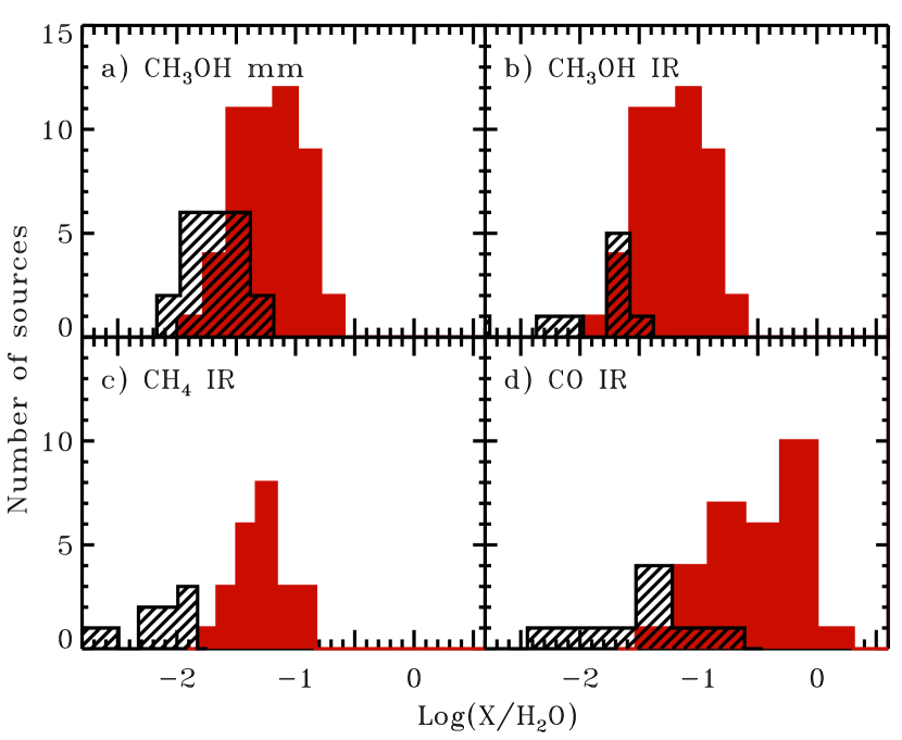
Figure 13: Comparison of low-mass protostellar (red solid) and comet (black lines) abundances with respect for water of CH₃OH, CH₄ and CO. The comet CH₃OH abundances in a) are based on millimeter observations from Biver et al. (2002). All other comet abundances are from IR observations compiled by Disanti & Mumma (2008).

The protostellar stage includes the formation of an accretion disk, which is the formation site of planetesimals and eventually planets. These disks are observed to have cold midplanes, where ices should be abundant. It is often difficult to study these disk ices directly because of confusion between disk ices and ices in foreground clouds (Pontoppidan et al., 2005). Comets in our own solar system should, however, carry a record of the ice composition in one such disk midplane. It is unknown whether cometary ices reformed in the disk or whether they are at least partly pre-solar or protosolar; recent models suggest that much of the original ice will in fact survive accretion from the envelope into the disk (Visser et al., 2009). Even if cometary ices originate from protosolar ices, the protostellar and protosolar ice abundance populations are not expected to overlap perfectly, since the comets originate around a single star, whereas the spread in protostellar ices show the differences in ice abundances between different protostars. Assuming that the protosun resembled one of the observed protostars, what can be addressed is the question of whether comet ice abundances are consistent with a protosolar origin or whether additional ice chemistry in the protosolar nebula is required to account for the observed abundances. In light of this, Figure 13 shows a comparison between cometary and low-mass protostellar CH₃OH, CH₄ and CO abundances with respect to H₂O (Biver et al., 2002; Disanti & Mumma, 2008, and references therein).

For all three ices, the cometary abundances are well below the median protostellar abundances. If the observed cometary ices are pre-solar, this comparison implies either that the ice composition in the protosolar envelope was similar to the most carbon-poor ices observed in the protostellar sample, or that some ice abundances with respect to H₂O were reduced in the solar nebula. Possible selective ice destruction processes include desorption of the most volatile ices and UV induced chemistry.

The spread in cometary ice abundances is comparable to the spread found between different protostellar sources, suggestive either of a primordial variation in ice abundances within the protosolar envelope or of ice processing in the solar nebula, or a combination of the two. Once a sample of cometary CO₂ ice abundances become available, the dominant source of variation should be possible to constrain, since CO₂ ice abundances vary little in the protostellar stage. Already, however, the low CH₄ abundances do suggest significant ice destruction during the disk stage, through chemistry or selective desorption. Similarly, comets are known to be significantly depleted in nitrogen, and the small number of comets with directly measured NH₃/H₂O ratios reveal a loss of NH₃ compared to low mass protostars (Kawakita & Mumma, 2011, and references therein) – suggesting that the alteration of cometary ices is not specifically related to carbon. For a more complete cometary ice sample, see upcoming review by Mumma & Charnley (2011, ARAA review, in press).

5 Conclusions

Large samples of ice sources spanning diverse environments, evolutionary stages and luminosities are necessary both to determine ‘typical’ ice abundances and to identify how ice processes depend on their environment. The main findings from combining the $c2d$ and other ice surveys carried out in a homogenous way are listed below:

1. The CO and CO₂ abundance medians relative to H₂O are both $\sim$29% toward low-mass YSOs, while CH₄, NH₃ and CH₃OH are more than a factor of five less abundant.

2. CO₂:H₂O, CH₄ and NH₃ abundances vary little with respect to H₂O, suggesting co-formation. In contrast, CO:H₂O, OCN^-, CO₂:CO and CH₃OH vary by factors 2–3 (lower to upper quartile) with respect to H₂O, indicative of a separate formation pathway from H₂O ice. Pure CO and CO₂ ice abundances vary even more, consistent with their sensitivity to protostellar heating.

3. Ice abundances toward background stars and protostars are similar except for a lack of features associated with ice heating, such as pure CO₂ ice, toward background stars. In particular, there is no evidence for a different range of CH₃OH and CO₂ ice abundances.

4. Protostellar ice abundances in nearby star-forming regions do not vary significantly between different clouds, except for a significantly lower pure CO abundances toward the protostars in Taurus.

5. Compared to low-mass YSOs, ice abundances toward high-mass YSOs are characterized by low levels of CO and CO₂ ice, which can be explained by ice heating. Low-mass protostars in the highly irradiated region IC 1396A have typical low-mass protostellar CO₂ ice abundances, confirming that the original ice conditions during low- and high-mass star formation are similar.

6. Correlation studies within the low-mass protostellar sample show a close association between CO, CO₂:CO, CO:H₂O and the XCN band, supporting the latter’s identification with OCN^-.

7. Combining the above information, ice formation can generally be divided into three stages: an early phase driven by atomic hydrogenation reactions in clouds, which are fast compared to cloud core formation time scales of $\sim$10⁵ years; a later CO-freeze-out dependent ice formation phase which takes place in the pre-stellar phase; and finally the protostellar phase where thermal and possibly UV processing shape the ice content.

8. Toward both low- and high-mass protostars and toward molecular clouds, an average of 8–16% of the total C, O and N are bound up in ices. Toward the most ice-rich source (IRS 51) 60–80% of the non-refractory C and O are in ices.

9. There is evidence for more complex ices toward both low- and high-mass protostars, e.g. HCOOH, CH₃CHO and/or C₂H₅OH, but high-resolution spectra toward more sources are required to confirm their presence and quantify their abundances.

Facilities: Spitzer, VLT, Keck

Figure 5: Histograms of CO and CO₂ components, otherwise as in Fig. 4.

Figure 9: Ice abundances at different distances from the Oph-F core with respect to H₂O ice. The 2175 cm^-1 abundances are scaled by 40 and the CO₂:CO abundances by 5 for clarity. The CO₂ values are taken from Paper II, rather than Pontoppidan (2006), which affects especially the CO₂:H₂O curve.

Table 1: Ice column densities, abundances and optical depths of the 5–7 $\mu$m complex components.

Source	N(H2O)	[NH3]	[CH3OH]	$\tau_{\rm C1}$ (5.84 $\mu$m)	$\tau_{\rm C2}$ (6.18 $\mu$m)	$\tau_{\rm C3}$ (6.76 $\mu$m)	$\tau_{\rm C4}$ (6.94 $\mu$m)	$\tau_{\rm C5}$ (broad)
	1017 cm-2	%	%
WL 12	22.1 $\pm$ 3.0	$<$3.8	$<$4.5	0.012$\pm$0.003	0.000$\pm$0.002	0.049$\pm$0.004	0.136$\pm$0.003	0.014$\pm$0.071
WL 6	41.7 $\pm$ 6.0	2.9 $\pm$ 0.4	$<$2.1	0.002$\pm$0.007	0.000$\pm$0.006	0.137$\pm$0.007	0.087$\pm$0.006	0.030$\pm$0.045
IRS 42	19.5 $\pm$ 2.0	$<$2.1	11.9 $\pm$ 1.1	–	–	–	–	–
IRS 43	31.5 $\pm$ 4.0	–	–	0.059$\pm$0.004	0.082$\pm$0.003	0.179$\pm$0.005	0.105$\pm$0.004	0.066$\pm$0.051
IRS 44	34.0 $\pm$ 4.0	3.7 $\pm$ 0.4	$<$1.6	0.080$\pm$0.005	0.089$\pm$0.004	0.135$\pm$0.005	0.201$\pm$0.004	0.004$\pm$0.086
Elias 32	17.9 $\pm$ 2.6	$<$5.2	12.4 $\pm$ 1.9	0.021$\pm$0.005	0.000$\pm$0.004	0.050$\pm$0.009	0.075$\pm$0.007	0.058$\pm$0.025
IRS 46	12.8 $\pm$ 2.0	5.1 $\pm$ 0.9	$<$4.1	0.018$\pm$0.004	0.002$\pm$0.004	0.076$\pm$0.005	0.066$\pm$0.004	0.000$\pm$0.023
VSSG17	17.0 $\pm$ 2.5	$<$3.1	6.9 $\pm$ 2.4	0.058$\pm$0.002	0.056$\pm$0.002	0.042$\pm$0.005	0.061$\pm$0.004	0.011$\pm$0.016
IRS 51	22.1 $\pm$ 3.0	2.4 $\pm$ 0.3	11.7 $\pm$ 0.9	0.042$\pm$0.003	0.036$\pm$0.002	0.074$\pm$0.003	0.060$\pm$0.002	0.000$\pm$0.012
IRS 63	20.4 $\pm$ 3.0	5.7 $\pm$ 1.3	$<$1.8	0.000$\pm$0.003	0.023$\pm$0.002	0.048$\pm$0.003	0.060$\pm$0.003	0.044$\pm$0.039

Table 2: Typical ice abundances toward low- and high-mass protostars and background stars.

Ice feature	Low-mass	High-mass	background
H2O	100	100	100
CO	29	13	31
CO2	29	13	38
CH3OH	3	4	4
NH3	5	5	$\cdots$
CH4	5	2	$\cdots$
XCNa	0.3	0.6	$\cdots$

^aXCN implies a band component securely identified with OCN^- and the nearby 2175 cm^-1 component, which this study suggests is also due to OCN^-.

Table 3: Abundance medians^a and lower and upper quartile values of ices and individual ice components with respect to H₂O ice

Ice feature	Low-mass	High-mass	background
H2O	100	100	100
CO	38${}^{61}_{20}$ (29)	13${}_{7}^{19}$	31
CO2	29${}^{35}_{22}$	13${}_{12}^{22}$	38${}_{32}^{41}$
CH3OH	7${}^{12}_{5}$ (3)	8${}_{8}^{16}$ (4)	8${}_{7}^{10}$ (4)
NH3	5${}^{6}_{4}$	16${}_{10}^{17}$ (5)	$\cdots$
CH4	5${}^{7}_{4}$	4${}_{2}^{4}$ (2)	$\cdots$
XCN	0.6${}^{0.8}_{0.2}$ (0.3)	0.8${}_{0.4}^{1.4}$ (0.6)	$\cdots$
pure CO	21${}_{7}^{36}$	3${}_{2}^{6}$	$\cdots$
CO:H2O	13${}_{7}^{19}$	10${}_{5}^{12}$	$\cdots$
CO:CO2	2${}_{1}^{3}$	1.3${}_{0.4}^{1.6}$ (0.3)	$\cdots$
pure CO2	2${}_{0.3}^{4}$	2${}_{1}^{2}$	$\cdots$
CO2:H2O	20${}_{15}^{23}$	9${}_{6}^{15}$	24
CO2:CO	5${}_{4}^{7}$	5${}_{2}^{6}$	6
CO2 shoulder	0.8${}_{0.4}^{1.1}$	1${}_{1}^{2}$	$\cdots$
OCN-	0.4${}_{0.3}^{0.4}$ (0.2)	0.6${}_{0.4}^{1.4}$	$\cdots$
2175 cm-1	0.3${}_{0.2}^{0.4}$ (0.2)	0.1${}_{0.1}^{0.1}$	$\cdots$
C1 (HCOOH + H2CO)b	2.5${}_{1.7}^{3.1}$	2.1${}_{2.0}^{2.8}$	2.8${}_{2.4}^{3.3}$
C2 (HCOO-+NH3)b	1.9${}_{1.3}^{2.8}$ (1.1)	1.3${}_{1.0}^{1.6}$	2.5${}_{1.3}^{3.3}$
C3 (NH${}_{4}^{+}$ + CH3OH)b	4.3 ${}_{3.0}^{4.7}$	4.3${}_{3.6}^{5.4}$	3.7${}_{3.4}^{4.7}$
C4 (NH${}_{4}^{+}$)b	2.3${}_{2.1}^{3.7}$	4.3${}_{2.9}^{5.0}$	2.1${}_{1.1}^{2.8}$
C5 (warm H2O + anions)b	1.5${}_{0.8}^{2.2}$ (0.9)	3.3${}_{0.8}^{6.3}$ (1.4)	$\cdots$

^aValues in parentheses include upper limits in the median calculation using survival analysis.
^bSince no single carrier the reported number is peak optical depth / ($N_{\rm H_{2}O}\times 10^{-20}\times 100$).

Table 4: Differences in CO and CO₂ shoulder medians toward different star forming associations

	Pure CO	CO2 shoulder
Ophiuchus	32	0.9
Serpens	38	1.8
CrA	29	1.8
Perseus	21	0.8
Taurus	7	0.5
Other	5	0.5
Complete sample	21	0.8

Table 5: The amount of C, O and N bound up in protostellar ices.

	Cice / Ctotal	Oice / Ototal	Nice / Ntotal		Cice / Cvol	Oice / Ovol	Nice / Nvol
Low-mass median	15%	16%	10%		27%	34%	10%
Low-mass max	46%	29%	35%		83%	61%	35%
High-mass median	8%	12%	12%		14%	25%	12%
High-mass max	18%	17%	22%		32%	36%	22%

Appendix A Ophiuchus NH₃ and CH₃OH spectra

Figure 14 shows the acquired Spitzer spectra for the nine young stellar objects in Ophiuchus that were added to the $c2d$ sample. The spectra are dominated by a broad silicate feature which is removed by fitting a polynomial to regions free of molecular emission and absorption. We used the same fitting regions as in Paper IV to determine the ice band depths and shapes and then shifted the regions by $\sim$0.1$\mu$m to determine the sensitivity of the results to the chosen local continuum.

The resulting optical depth spectra are shown in Fig. 15. CH₃OH ice is detected toward Elias 32, IRS 42, IRS 51 and VSSG 17 and NH₃ ice toward IRS 44, IRS 46, IRS 51, IRS 63 and WL 6. The bands are fitted with Gaussians and the derived peak positions and full-width-half-maxima are listed in Table 6. The uncertainties are dominated by the choice of local continuum. The NH₃ peak positions are consistent with laboratory ice spectra, while the FWHM are generally too low. From Paper IV, we know that the NH₃ FWHM may be underestimated when using a local continuum rather than a silicate template to extract optical depth spectra and this explains the discrepancy. The CH₃OH peak positions and FWHM are both consistent with laboratory measurements, with the peak positions suggesting that CH₃OH is present in a CO-rich ice (Paper IV).

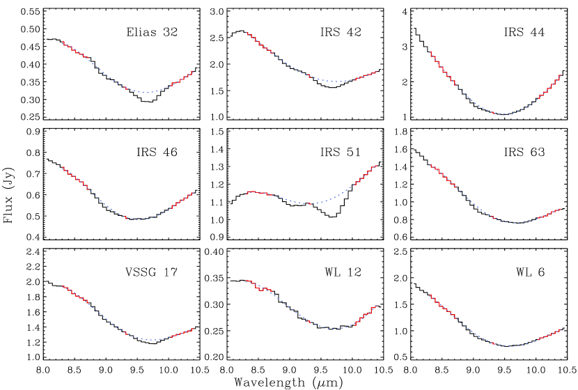
Figure 14: Spitzer spectra between 8.0 and 10.5 $\mu$m showing the silicate feature and the superimposed bands at 9 and 9.7 $\mu$m ascribed to NH₃ and CH₃OH ice, respectively. The red regions were used to fit a local continuum (blue dotted line).

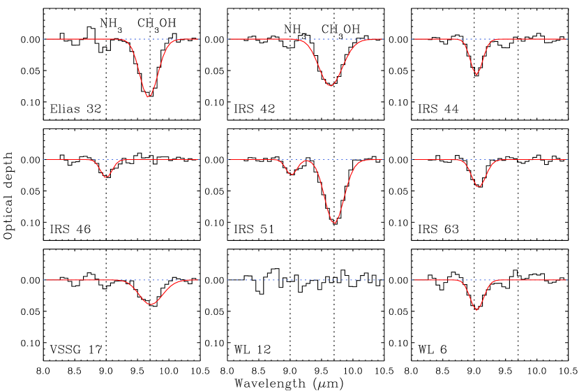
Figure 15: Optical depth spectra of NH₃ and CH₃OH ice features toward the Ophiuchus sources obtained after subtracting the silicate feature. The red line shows the Gaussian fits to the detected bands.

Table 6: FWHM and peak positions of detected NH₃ and CH₃OH bands compared to laboratory values.

Source	Peak position NH3		FWHM NH3	Peak position CH3OH		FWHM CH3OH
	$\mu$m	cm-1	cm-1	$\mu$m	cm-1	cm-1
Elias 32	$\cdots$	$\cdots$	$\cdots$	9.68$\pm 0.01$	1033$\pm$1	36 $\pm$ 3
IRS 42	$\cdots$	$\cdots$	$\cdots$	9.64$\pm$0.01	1037$\pm$1	47 $\pm$ 3
IRS 44	9.04$\pm$0.01	1107$\pm$1	28 $\pm$ 2	$\cdots$	$\cdots$	$\cdots$
IRS 46	9.00$\pm$0.01	1110$\pm$1	27 $\pm$ 3	$\cdots$	$\cdots$	$\cdots$
IRS 51	9.02$\pm$0.01	1109$\pm$1	25 $\pm$ 1	9.70$\pm$0.01	1031$\pm$1	38 $\pm$ 2
IRS 63	9.07$\pm$0.02	1102$\pm$2	32 $\pm$ 5	$\cdots$	$\cdots$	$\cdots$
VSSG 17	$\cdots$	$\cdots$	$\cdots$	9.71$\pm$0.02	1030$\pm$3	45 $\pm$ 10
WL 12	$\cdots$	$\cdots$	$\cdots$	$\cdots$	$\cdots$	$\cdots$
WL 6	9.04$\pm$0.01	1106$\pm$1	31 $\pm$ 2	$\cdots$	$\cdots$	$\cdots$
Laboratorya	8.85–9.41	1062–1130	53–137	9.67–9.83	1017–1034	22–39

^aBottinelli et al. (2010)

Appendix B Carriers of the 7.25 $\mu$m ice feature

Paper I showed that it is difficult to fit the 7.25 $\mu$m with spectra of HCOOH, its most commonly assigned carrier. Laboratory spectra of some tertiary mixtures come closest, but suffer from uncertainties in baseline determinations (see below).

Figure 16 shows the spectra of pure HCOOH ice and an H₂O:HCOOH 4:1 ice mixture (at 15 K from Bisschop et al., 2007)), pure CH₃CH₂OH and CH₃CHO spectra (Öberg et al., 2009b), and observed spectra toward W33A, NGC7538 IRS9 and B1-b. W33A and B1-b clearly have absorption features at 7.25 and 7.4 $\mu$m, while NGC7538 IRS9 does not. The comparison shows that CH₃CH₂OH is a plausible carrier for the 7.25 $\mu$m feature, commonly assigned to HCOOH. The lack of the 7.25 $\mu$m toward NGC7538 IRS9 is consistent with the upper limit on CH₃CH₂OH ice from the 3 $\mu$m feature (Boudin et al., 1998), while no such limits are published for the other sources. Figure 16 also shows that the observed 7.40 $\mu$m feature is likely due to CH₃CHO. Thus there is also little evidence for HCOO^- – both have been proposed previously as carriers (e.g. Schutte et al., 1999; Gibb et al., 2004, Paper I).

These tentative identifications may in the future provide an opportunity to observe a complex ice chemistry in situ, but the Spitzer-IRS spectra are too low in spectral resolution to securely distinguish between different carriers, especially since the HCOOH spectral feature depends on the ice matrix and has been reported to become as narrow as the CH₃CH₂OH band in mixtures with H₂O and CH₃OH, but this result depends crucially on the choice of local baseline (Bisschop et al., 2007). Until the HCOOH baseline issue has been resolved and higher resolution spectra exist for more sources the HCOOH and HCOO^- abundances should not be determined from the 7.25 and 7.42 $\mu$m ice features. This does not imply that HCOOH and HCOO^- are not present in interstellar ices, only that we do not currently have the tools to quantify their abundances.

Figure 16: ISO spectra at 7–8 $\mu$m for W33A, NGC7538 IRS9 and B1-b, following subtraction of a local spline continuum, plotted together with laboratory spectra of pure HCOOH, CH₃CHO and CH₃CH₂OH ices. The dashed lines mark the 7.25 and 7.40 $\mu$m features usually assigned to HCOOH and HCOO^-. The feature at 7.67 $\mu$m is due to CH₄ ice. The baselines were obtained by fitting a local spline continuum to 6.9, 7.16, 7.33, 7.77 and 7.85 $\mu$m.

Appendix C Histograms of ice detections and detections$+$upper limits

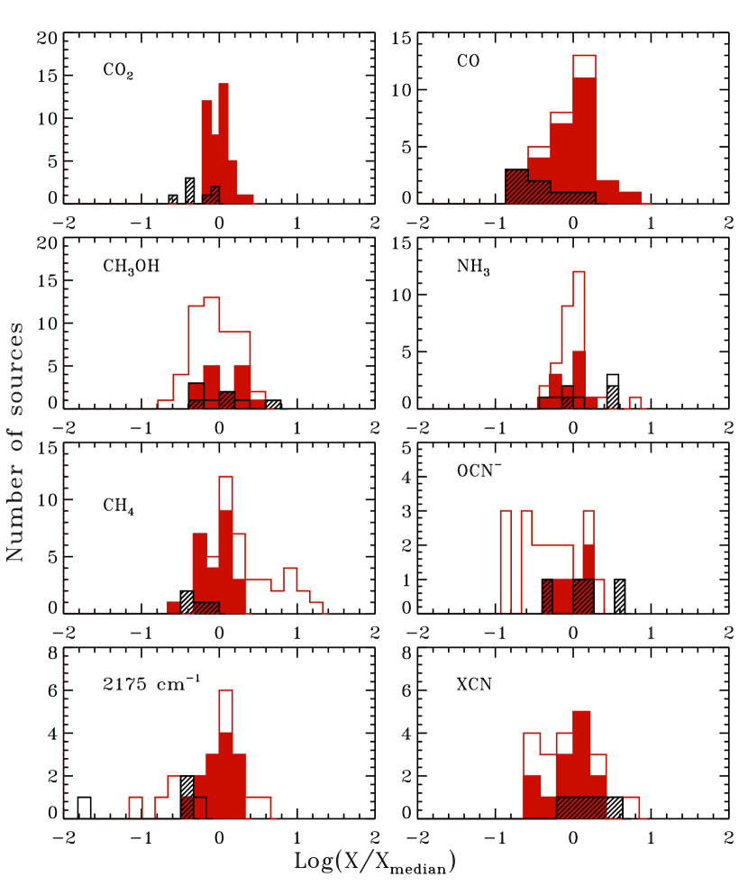
Figure 17: Histograms of total ice abundances toward low-mass protostars (red) and high-mass protostars (black). Solid histograms mark detections and contours detections$+$upper limits. For low-mass NH₃ the solids are from Paper IV using a silicate template to extract NH₃ and the contour are from Paper IV and Table 1 when using a polynomial to fit the local continuum.

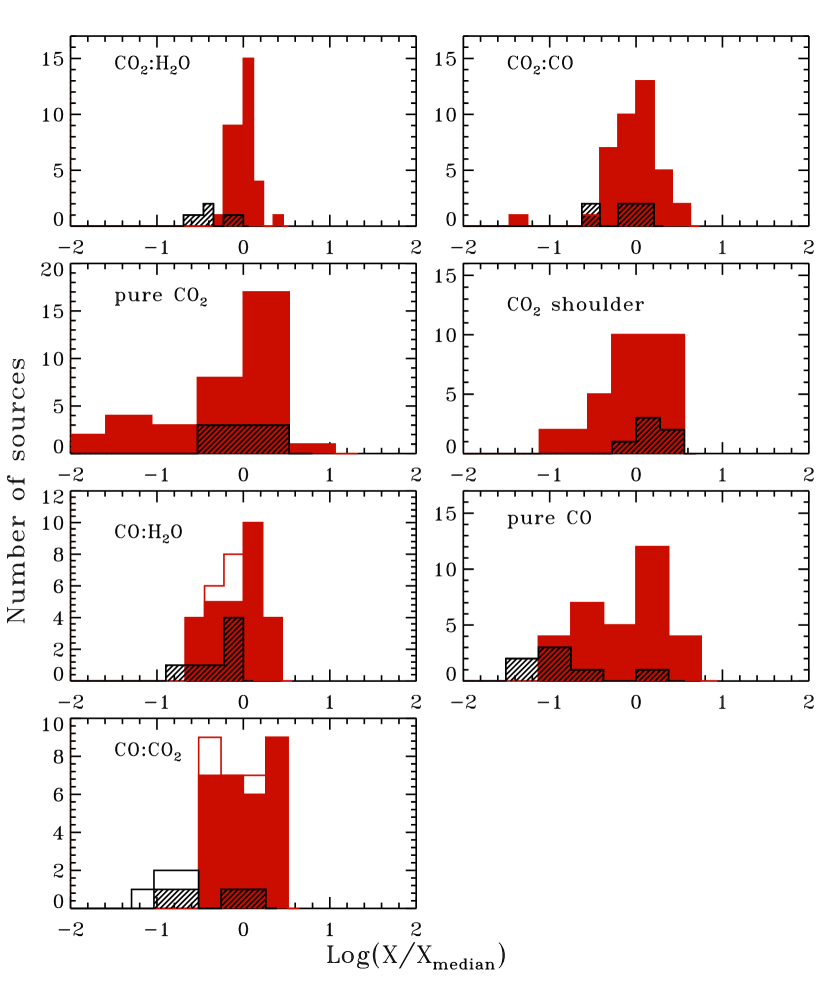
Figure 18: Histograms of CO and CO₂ components, otherwise as in Fig. 17

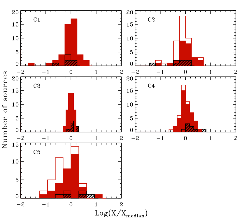
Figure 19: Histograms of 5-7 $\mu$m components, otherwise as in Fig. 17.

References

- An et al. (2009) An, D., Ramírez, S. V., Sellgren, K., et al. 2009, ApJ, 702, L128
- Bergin et al. (2005) Bergin, E. A., Melnick, G. J., Gerakines, P. A., Neufeld, D. A., & Whittet, D. C. B. 2005, ApJ, 627, L33
- Bisschop et al. (2007) Bisschop, S. E., Fuchs, G. W., van Dishoeck, E. F., & Linnartz, H. 2007, A&A, 474, 1061
- Biver et al. (2002) Biver, N., Bockelée-Morvan, D., Crovisier, J., et al. 2002, Earth Moon and Planets, 90, 323
- Bohlin et al. (1978) Bohlin, R. C., Savage, B. D., & Drake, J. F. 1978, ApJ, 224, 132
- Boogert & Ehrenfreund (2004) Boogert, A. C. A. & Ehrenfreund, P. 2004, in ASP Conf. Ser. 309: Astrophysics of Dust, ed. A. N. Witt, G. C. Clayton, & B. T. Draine, 547–572
- Boogert et al. (2011) Boogert, A. C. A., Huard, T. L., Cook, A. M., et al. 2011, ApJ, 729, 92
- Boogert et al. (2008) Boogert, A. C. A., Pontoppidan, K. M., Knez, C., et al. 2008, ApJ, 678, 985
- Boogert et al. (2004) Boogert, A. C. A., Pontoppidan, K. M., Lahuis, F., et al. 2004, ApJS, 154, 359
- Bottinelli et al. (2010) Bottinelli, S., Adwin Boogert, A. C., Bouwman, J., et al. 2010, ApJ, 718, 1100
- Boudin et al. (1998) Boudin, N., Schutte, W. A., & Greenberg, J. M. 1998, A&A, 331, 749
- Charnley et al. (1992) Charnley, S. B., Tielens, A. G. G. M., & Millar, T. J. 1992, ApJ, 399, L71
- Chiar et al. (1995) Chiar, J. E., Adamson, A. J., Kerr, T. H., & Whittet, D. C. B. 1995, ApJ, 455, 234
- Chiar et al. (2007) Chiar, J. E., Ennico, K., Pendleton, Y. J., et al. 2007, ApJ, 666, L73
- Collings et al. (2004) Collings, M. P., Anderson, M. A., Chen, R., et al. 2004, MNRAS, 354, 1133
- Cuppen et al. (2009) Cuppen, H. M., van Dishoeck, E. F., Herbst, E., & Tielens, A. G. G. M. 2009, A&A, 508, 275
- Dartois et al. (1999) Dartois, E., Demyk, K., d’Hendecourt, L., & Ehrenfreund, P. 1999, A&A, 351, 1066
- Disanti & Mumma (2008) Disanti, M. A. & Mumma, M. J. 2008, Space Sci. Rev., 138, 127
- Dunham et al. (2010) Dunham, M. M., Evans, N. J., Bourke, T. L., et al. 2010, ApJ, 721, 995
- Ehrenfreund et al. (1992) Ehrenfreund, P., Breukers, R., D’Hendecourt, L., & Greenberg, J. M. 1992, A&A, 260, 431
- Evans et al. (2009) Evans, N. J., Dunham, M. M., Jørgensen, J. K., et al. 2009, ApJS, 181, 321
- Evans et al. (2003) Evans, II, N. J., Allen, L. E., Blake, G. A., et al. 2003, PASP, 115, 965
- Fayolle et al. (2011) Fayolle, E. C., Öberg, K. I., Cuppen, H. M., Visser, R., & Linnartz, H. 2011, A&A, 529, A74+
- Feigelson & Nelson (1985) Feigelson, E. D. & Nelson, P. I. 1985, ApJ, 293, 192
- Fuchs et al. (2006) Fuchs, G. W., Acharyya, K., Bisschop, S. E., et al. 2006, Faraday Discussions, 133, 331
- Garrod & Pauly (2011) Garrod, R. T. & Pauly, T. 2011, ArXiv e-prints
- Garrod et al. (2008) Garrod, R. T., Weaver, S. L. W., & Herbst, E. 2008, ApJ, 682, 283
- Gibb et al. (2004) Gibb, E. L., Whittet, D. C. B., Boogert, A. C. A., & Tielens, A. G. G. M. 2004, ApJS, 151, 35
- Gibb et al. (2000) Gibb, E. L., Whittet, D. C. B., Schutte, W. A., et al. 2000, ApJ, 536, 347
- Gillett & Forrest (1973) Gillett, F. C. & Forrest, W. J. 1973, ApJ, 179, 483
- Goldsmith et al. (2000) Goldsmith, P. F., Melnick, G. J., Bergin, E. A., et al. 2000, ApJ, 539, L123
- Ioppolo et al. (2009) Ioppolo, S., Palumbo, M. E., Baratta, G. A., & Mennella, V. 2009, A&A, 493, 1017
- Ioppolo et al. (2011) Ioppolo, S., van Boheemen, Y., Cuppen, H. M., van Dishoeck, E. F., & Linnartz, H. 2011, MNRAS, 238
- Kawakita & Mumma (2011) Kawakita, H. & Mumma, M. J. 2011, ApJ, 727, 91
- Keane et al. (2001) Keane, J. V., Boonman, A. M. S., Tielens, A. G. G. M., & van Dishoeck, E. F. 2001, A&A, 376, L5
- Kim et al. (2011a) Kim, H. J., Evans, II, N. J., Dunham, M. M., et al. 2011a, ApJ, 729, 84
- Kim et al. (2011b) Kim, H. J., Evans, II, N. J., Dunham, M. M., & Lee, J. E. 2011b, in IAU Symposium, Vol. 280, IAU Symposium, 216P–+
- Knez et al. (2005) Knez, C., Boogert, A. C. A., Pontoppidan, K. M., et al. 2005, ApJ, 635, L145
- Kruskal & Wallis (1952) Kruskal, W. H. & Wallis, W. A. 1952, Journal of the American Statistical Association, 47, pp. 583
- McLean et al. (1998) McLean, I. S., Becklin, E. E., Bendiksen, O., et al. 1998, in Society of Photo-Optical Instrumentation Engineers (SPIE) Conference Series, ed. A. M. Fowler, Vol. 3354, 566–578
- Merrill et al. (1976) Merrill, K. M., Russell, R. W., & Soifer, B. T. 1976, ApJ, 207, 763
- Meyer et al. (1998) Meyer, D. M., Jura, M., & Cardelli, J. A. 1998, ApJ, 493, 222
- Moorwood (1997) Moorwood, A. F. 1997, in Society of Photo-Optical Instrumentation Engineers (SPIE) Conference Series, ed. A. L. Ardeberg, Vol. 2871, 1146–1151
- Oba et al. (2010) Oba, Y., Watanabe, N., Kouchi, A., Hama, T., & Pirronello, V. 2010, ApJ, 712, L174
- Öberg (2009) Öberg, K. I. 2009, PhD thesis, Leiden Observatory, Leiden University
- Öberg et al. (2008) Öberg, K. I., Boogert, A. C. A., Pontoppidan, K. M., et al. 2008, ApJ, 678, 1032
- Öberg et al. (2009a) Öberg, K. I., Fayolle, E. C., Cuppen, H. M., van Dishoeck, E. F., & Linnartz, H. 2009a, A&A, 505, 183
- Öberg et al. (2009b) Öberg, K. I., Garrod, R. T., van Dishoeck, E. F., & Linnartz, H. 2009b, A&A, 504, 891
- Oliveira et al. (2011) Oliveira, J. M., van Loon, J. T., Sloan, G. C., et al. 2011, MNRAS, 411, L36
- Pagani et al. (2003) Pagani, L., Olofsson, A. O. H., Bergman, P., et al. 2003, A&A, 402, L77
- Pendleton et al. (1999) Pendleton, Y. J., Tielens, A. G. G. M., Tokunaga, A. T., & Bernstein, M. P. 1999, ApJ, 513, 294
- Pontoppidan (2006) Pontoppidan, K. M. 2006, A&A, 453, L47
- Pontoppidan et al. (2008) Pontoppidan, K. M., Boogert, A. C. A., Fraser, H. J., et al. 2008, ApJ, 678, 1005
- Pontoppidan et al. (2003a) Pontoppidan, K. M., Dartois, E., van Dishoeck, E. F., Thi, W., & d’Hendecourt, L. 2003a, A&A, 404, L17
- Pontoppidan et al. (2005) Pontoppidan, K. M., Dullemond, C. P., van Dishoeck, E. F., et al. 2005, ApJ, 622, 463
- Pontoppidan et al. (2003b) Pontoppidan, K. M., Fraser, H. J., Dartois, E., et al. 2003b, A&A, 408, 981
- Pontoppidan et al. (2004) Pontoppidan, K. M., van Dishoeck, E. F., & Dartois, E. 2004, A&A, 426, 925
- Przybilla et al. (2008) Przybilla, N., Nieva, M., & Butler, K. 2008, ApJ, 688, L103
- Raunier et al. (2003) Raunier, S., Chiavassa, T., Marinelli, F., Allouche, A., & Aycard, J.-P. 2003, J. Phys. Chem. A, 107, 9335
- Reach et al. (2009) Reach, W. T., Faied, D., Rho, J., et al. 2009, ApJ, 690, 683
- Roche & Aitken (1985) Roche, P. F. & Aitken, D. K. 1985, MNRAS, 215, 425
- Sandford & Allamandola (1990) Sandford, S. A. & Allamandola, L. J. 1990, ApJ, 355, 357
- Schutte et al. (1999) Schutte, W. A., Boogert, A. C. A., Tielens, A. G. G. M., et al. 1999, A&A, 343, 966
- Schutte & Khanna (2003) Schutte, W. A. & Khanna, R. K. 2003, A&A, 398, 1049
- Shen et al. (2004) Shen, C. J., Greenberg, J. M., Schutte, W. A., & van Dishoeck, E. F. 2004, A&A, 415, 203
- Spearman (1904) Spearman, C. 1904, The American Journal of Psychology, 15, pp. 72
- Tielens & Hagen (1982) Tielens, A. G. G. M. & Hagen, W. 1982, A&A, 114, 245
- Tielens et al. (1991) Tielens, A. G. G. M., Tokunaga, A. T., Geballe, T. R., & Baas, F. 1991, ApJ, 381, 181
- Turner et al. (1999) Turner, B. E., Terzieva, R., & Herbst, E. 1999, ApJ, 518, 699
- van Breemen et al. (2011) van Breemen, J. M., Min, M., Chiar, J. E., et al. 2011, A&A, 526, A152+
- van Broekhuizen et al. (2004) van Broekhuizen, F. A., Keane, J. V., & Schutte, W. A. 2004, A&A, 415, 425
- van Broekhuizen et al. (2005) van Broekhuizen, F. A., Pontoppidan, K. M., Fraser, H. J., & van Dishoeck, E. F. 2005, A&A, 441, 249
- van der Tak et al. (2000) van der Tak, F. F. S., van Dishoeck, E. F., Evans, II, N. J., & Blake, G. A. 2000, ApJ, 537, 283
- Vandenbussche et al. (1999) Vandenbussche, B., Ehrenfreund, P., Boogert, A. C. A., et al. 1999, A&A, 346, L57
- Visser et al. (2009) Visser, R., van Dishoeck, E. F., Doty, S. D., & Dullemond, C. P. 2009, A&A, 495, 881
- Weingartner & Draine (2001) Weingartner, J. C. & Draine, B. T. 2001, ApJ, 548, 296
- Whittet (2010) Whittet, D. C. B. 2010, ApJ, 710, 1009
- Whittet et al. (1988) Whittet, D. C. B., Bode, M. F., Longmore, A. J., et al. 1988, MNRAS, 233, 321
- Whittet et al. (2009) Whittet, D. C. B., Cook, A. M., Chiar, J. E., et al. 2009, ApJ, 695, 94
- Whittet et al. (2007) Whittet, D. C. B., Shenoy, S. S., Bergin, E. A., et al. 2007, ApJ, 655, 332
- Zasowski et al. (2009) Zasowski, G., Kemper, F., Watson, D. M., et al. 2009, ApJ, 694, 459