SCET, QCD and Wilson Lines

Abstract:

Soft Collinear Effective Theory (SCET) is an effective field theory which describes the interactions of low invariant mass jets which are highly boosted with respect to one another. In the standard formulation of SCET, the effective Lagrangian for collinear fields is expanded in inverse powers of the energy. At leading order this leads to manifest decoupling of soft and collinear degrees of freedom; however, subleading terms in the effective Lagrangian violate this manifest decoupling. In this paper we point out that the collinear expansion in the SCET Lagrangian is unnecessary, and that the SCET Lagrangian may instead be written as multiple decoupled copies of QCD. The interactions between the sectors in full QCD are reproduced in the effective theory by an external current consisting of QCD fields coupled to Wilson lines. We illustrate this picture with two examples: dijet production and $B\to X_{s}\gamma$.

1 Introduction

Soft-Collinear Effective Theory (SCET) [1, 2, 3, 4, 5, 6] describes the interaction of low invariant mass jets of particles which are highly boosted with respect to one another. SCET is an expansion in inverse powers of the highly boosted energy. At leading order in the SCET expansion, a field redefinition may be used to manifestly decouple the soft and collinear degrees of freedom from one another at the operator level [4]. Interactions between different soft and collinear sectors are reproduced in the currents of the effective theory by lightlike Wilson lines. This simplification is the basis of factorization theorems in SCET, allowing differential cross sections to be written as convolutions of independent soft and collinear pieces. While factorization theorems have been well-studied using traditional QCD approaches, the manifest decoupling of soft and collinear pieces at the level of the Lagrangian in SCET both dramatically simplifies the study of factorization theorems, and allows power corrections in inverse energy to be studied in a systematic way.

In standard formulations of SCET [1, 2, 3, 4, 5, 6, 7], there is an inherent asymmetry in the treatment of soft and collinear degrees of freedom. While, for example, soft quark fields are identical to four-component QCD quark fields, collinear quark fields are described by two-component spinors with complicated nonlocal interactions. On general grounds, this asymmetry must be spurious: QCD is Lorentz invariant, and dimensional regularization is a Lorentz invariant regulator. One may therefore always boost to a reference frame in which the energy of the collinear fields is small, and the collinear quark fields are described by four-component QCD fields. Thus, the SCET description of collinear fields must be equivalent to that of full QCD.

This is not a new observation. It was observed in [6] that the Feynman rules of collinear SCET fields are equivalent to those of QCD in light-cone quantization [8], and this equivalence has been used to simplify calculations in the collinear sector of the theory [1, 2, 9]. In [10], it was formally proven at leading order in power corrections that SCET is equivalent to multiple copies of QCD coupled to Wilson lines when the field redefinition of [4] is used to decouple soft from collinear fields. However, beyond leading order the approach was less clear.

In this paper, we argue that this picture may be extended to all orders in the SCET expansion. We show that the soft and collinear sectors of SCET may individually be described by a separate copy of the full QCD Lagrangian, and that these sectors are decoupled from one another to all orders in the SCET expansion. The interactions between the sectors in full QCD are reproduced by the interactions between the individual sectors and the external current, which consists of QCD fields coupled to Wilson lines. In particular, soft-collinear mixing terms in the Lagrangian do not arise in the theory; their effects are accounted for by subleading corrections to the external current, whose form is similar to that of subleading twist shape functions [11, 12].

In order to motivate this picture, we derive the subleading operators for two specific phenomena; $e^{+}e^{-}\to$ dijet production and $B\to X_{s}\gamma$. In Sec. 2 we review the standard derivation of SCET. In Sec. 3.1 we present our approach for dijet production at leading order, while in Sec. 3.2 we derive the new subleading operators for dijet production. In Sec. 4 we present a similar analysis for $B\to X_{s}\gamma$, and in Sec. 5 we present our conclusions.

2 Label SCET Formulation

In the approach to SCET introduced in [1, 2, 3, 4, 5], collinear fields are described by effective two-component spinors, $\xi_{n,\tilde{p}}$, where $n$ denotes the (lightlike) direction of motion, $\tilde{p}$ is a label which denotes the large components of the collinear momentum,

$$\tilde{p}^{\mu}\equiv{\bar{n}}\cdot p\,\frac{n^{\mu}}{2}+p_{\perp}^{\mu}$$ (1)

and the collinear quark momentum is $p^{\mu}=\tilde{p}^{\mu}+k^{\mu}$. We will refer to this approach as “label SCET” to denote the removal of the large label momentum, and to distinguish it from the approach of [6, 7], in which label momentum was not removed, but the collinear quarks were still treated as two-component spinors. The SCET Lagrangian for the collinear quark field is obtained by integrating out the two small components of the field and expanding in powers of $\lambda^{2}\sim k^{\mu}/{\bar{n}}\cdot p$. This procedure results in the effective Lagrangian for the $n$-collinear quark

$${\cal L}_{\xi}={\cal L}^{(0)}_{\xi\xi}+{\cal L}^{(1)}_{\xi\xi}+{\cal L}^{(1)}_{\xi q}+\ldots,$$ (2)

where the superscript refers to the suppression in $\lambda$ [6, 7, 13, 14, 15, 16]. The leading order term ${\cal L}_{\xi\xi}^{(0)}$ is

$${\cal L}_{\xi\xi}^{(0)} = \sum_{\tilde{p},\tilde{p}^{\prime}}\bar{\xi}_{n,\tilde{p}^{\prime}}\left[in\cdot D+i\mathchoice{\ooalign{$\hfil\displaystyle\mkern 0.0mu/\hfil$\crcr$\displaystyle D$}}{\ooalign{$\hfil\textstyle\mkern 0.0mu/\hfil$\crcr$\textstyle D$}}{\ooalign{$\hfil\scriptstyle\mkern 0.0mu/\hfil$\crcr$\scriptstyle D$}}{\ooalign{$\hfil\scriptscriptstyle\mkern 0.0mu/\hfil$\crcr$\scriptscriptstyle D$}}^{\perp}_{n}W_{n}\frac{1}{{\bar{n}}\cdot{\cal P}}W_{n}^{\dagger}i\mathchoice{\ooalign{$\hfil\displaystyle\mkern 0.0mu/\hfil$\crcr$\displaystyle D$}}{\ooalign{$\hfil\textstyle\mkern 0.0mu/\hfil$\crcr$\textstyle D$}}{\ooalign{$\hfil\scriptstyle\mkern 0.0mu/\hfil$\crcr$\scriptstyle D$}}{\ooalign{$\hfil\scriptscriptstyle\mkern 0.0mu/\hfil$\crcr$\scriptscriptstyle D$}}^{\perp}_{n}\right]\frac{\mathchoice{\ooalign{$\hfil\displaystyle\mkern 0.0mu/\hfil$\crcr$\displaystyle\bar{n}$}}{\ooalign{$\hfil\textstyle\mkern 0.0mu/\hfil$\crcr$\textstyle\bar{n}$}}{\ooalign{$\hfil\scriptstyle\mkern 0.0mu/\hfil$\crcr$\scriptstyle\bar{n}$}}{\ooalign{$\hfil\scriptscriptstyle\mkern 0.0mu/\hfil$\crcr$\scriptscriptstyle\bar{n}$}}}{2}\xi_{n,\tilde{p}}$$ (27)

where the covariant derivative $D_{\mu}=\partial_{\mu}-igT^{a}A_{\mu}^{a}$, $A^{\mu}=A^{\mu}_{s}+A^{\mu}_{n}$ contains both soft and collinear gluons, $D_{n}^{\mu}$ only contains $n$-collinear gluons, $W_{n}$ is a Wilson line built out of collinear $A_{n}$ fields in the ${\bar{n}}$ direction, and the “label operator” ${\cal P}^{\mu}$ pulls down the large label momentum of the collinear fields. The subleading operator ${\cal L}_{\xi\xi}^{(1)}$ describes higher order corrections to the interactions in ${\cal L}_{\xi\xi}^{(0)}$, while the subleading operator ${\cal L}_{\xi q}^{(1)}$ is the leading operator which couples collinear and soft quarks. Performing the field redefinitions on collinear quark and gluon fields [4]

$$\xi_{n,\tilde{p}}(x) = Y_{n}^{(\bf 3)}(x,\infty)\xi_{n,\tilde{p}}^{(0)}(x)$$

$$A_{n,\tilde{p}}^{a\,\mu}(x) = Y_{n}^{(\bf 8)}{}^{ab}(x,\infty)A_{n,\tilde{p}}^{(0)\,b\,\mu}(x),$$ (28)

where $Y_{n}^{{(\bf R)}}$ are Wilson lines built out of soft $A_{s}$ fields defined below, it may be shown that all dependence on soft gluons disappears from the leading order Lagrangian (27), so soft and collinear fields manifestly decouple at leading order in SCET. The collinear and soft lightlike Wilson lines in position space are defined as

$$W^{(\bf R)}_{n}(x,y) = P\exp\left(-ig\int_{0}^{\frac{n}{2}\cdot(y-x)}ds\,{\bar{n}}\cdot A^{a}_{n}(x+{\bar{n}}s)T_{\bf R}^{a}\right)$$

$$Y^{(\bf R)}_{n}(x,y) = P\exp\left(-ig\int_{0}^{\frac{{\bar{n}}}{2}\cdot(y-x)}ds\,n\cdot A^{a}_{s}(x+ns)T_{\bf R}^{a}\right)$$ (29)

where ${\bf R}$ labels the $SU(3)$ representation. Under a gauge transformation, the Wilson lines transform as

$$W_{n}^{(\bf R)}(x,y)\to\mathcal{U}_{c}^{(\bf R)}(x)W_{n}^{(\bf R)}(x,y)\mathcal{U}_{c}^{{(\bf R)}\dagger}(y)$$

$$Y_{n}^{(\bf R)}(x,y)\to\mathcal{U}_{s}^{(\bf R)}(x)Y_{n}^{(\bf R)}(x,y)\mathcal{U}_{s}^{{(\bf R)}\dagger}(y)$$ (30)

where $\mathcal{U}_{c,s}^{{(\bf R)}}$ is either a collinear or soft gauge transformation for representation ${\bf R}$. Note that $W_{n}^{{(\bf R)}}(x,y)=W_{n}^{{(\bf R)}\dagger}(y,x)$, and similarly for $Y_{n}^{{(\bf R)}}$, and that $W_{n}^{(\bf R)}(x,y)$ and $Y_{n}^{(\bf R)}(x,y)$ correspond to colour charge $\bf R$ propagating from $y$ to $x$. Also note that $W_{n}^{(\bf R)}$ and $Y_{n}^{(\bf R)}$ couple the ${\bar{n}}$ and $n$ components of the corresponding gluons, respectively; this notation is used to be consistent with the SCET literature.

At leading order, performing the field redefinitions (2), the current for dijet production in the full theory

$${\cal J}_{2}^{\rm QCD}=e^{-iQ\cdot x}\;\bar{\psi}(x)\Gamma\psi(x)$$ (31)

(where $\Gamma$ is an arbitrary Dirac structure and $Q$ is the external momentum) may be written in the factorized form in the effective theory

$$\tilde{\cal J}^{(0)}_{2}=e^{-iQ\cdot x}\;\bar{\xi}^{(0)}_{n,\tilde{p}_{1}}(x)W_{n}^{(\bf 3)}(x,\infty)Y_{n}^{(\bf 3)}{}^{\dagger}(x,\infty)\Gamma Y_{\bar{n}}^{(\bf 3)}(x,\infty)W_{\bar{n}}^{(\bf 3)}{}^{\dagger}(x,\infty)\xi^{(0)}_{{\bar{n}},\tilde{p}_{2}}(x)$$ (32)

where the $W_{\bar{n}}$ and $Y_{\bar{n}}$’s are lightlike Wilson lines defined analogously to (2). Label momentum conservation is enforced at each vertex. The collinear Wilson line $W_{n}^{(\bf 3)}$ arises from integrating out the interactions of $n$-collinear  fields with $\bar{n}$-collinear fields and similarly for $W_{\bar{n}}^{(\bf 3)}$. Each sector is therefore decoupled at leading order and described by QCD fields coupled to Wilson lines.

In this form it is manifest that all interactions between the different sectors occur via Wilson lines, as was formally shown in [10]. The redefined quark fields $\xi^{(0)}$ do not transform under soft gauge transformations, so the soft fields only couple to the Wilson line $Y$. Physically, this corresponds to the fact that soft fields cannot deflect the worldline of a highly energetic quark, and so they only see the direction and gauge charge of the collinear degrees of freedom (much the same way that in Heavy Quark Effective Theory [17], soft degrees of freedom only see the velocity and gauge charge of heavy quarks). Similarly, in a frame in which the $n$-collinear quark fields are soft, the soft and $\bar{n}$-collinear fields are recoiling in the opposite direction; thus the $n$-collinear quark fields can only resolve the total gauge charge of the combined soft and $\bar{n}$-collinear fields via the Wilson line $W_{n}$ (and similarly for the $\bar{n}$-collinear fields).

At higher orders in the expansion, however, label SCET looks more complicated, and the operator decoupling is no longer manifest. In particular, interactions such as ${\cal L}_{\xi q}^{(1)}$, in which soft and collinear sectors couple directly instead of via Wilson lines [15], make the extension of the arguments in [10] to higher orders unclear. In the next section we show how the leading order picture can be easily extended, by reformulating the theory using QCD fields.

Another formulation of SCET [6, 7] replaces the removal of label momentum with a multipole expansion in soft position. Our formulation of SCET more closely resembles this formulation than label SCET. However, we will diverge from the [6, 7] treatment of collinear quarks, which are two-component spinors giving mixed collinear-soft Lagrangian terms at subleading orders similar to label SCET. Also, the non-Abelian nature of SCET requires the introduction of a Wilson line $R(x)$ [7]. Without the $R$ Wilson line, soft transformations of collinear fields gives higher order in $\lambda$ pieces due to the soft and collinear fields being at different positions. The $R$ Wilson line redefines the collinear fields so they transform homogeneously in $\lambda$ under soft transformations. However, after the field redefinition (2), collinear fields no longer transform under the soft gauge group, and the $R$ Wilson line is not needed. In our formulation, soft and collinear fields are decoupled and each sector does not transform under the other so the $R$ Wilson line will be unneeded.

3 SCET as QCD Fields Coupled to Wilson Lines

Despite the complexity of the leading order $n$-collinear Lagrangian (27) and the corresponding Feynman rules, it is equivalent to the QCD Lagrangian [10, 6]. This is not unexpected: as long as one is just describing soft fields or collinear fields in one direction, there is no Lorentz-invariant expansion parameter, and one could just as easily work in a frame where the energy is small, in which case it is obvious that there is no effective field theory description and QCD is the appropriate theory. The large boost of a collinear quark only has physical meaning when it is coupled to fields with large relative momentum via an external current, such as in $e^{+}e^{-}\to q\bar{q}X$ or $B\to X_{s}\gamma$. The purpose of SCET is to describe the interactions in such situations between fields whose relative momentum is greater than the cutoff of the theory.

We therefore begin with the starting point that in the absence of an external current, each sector (collinear in each relevant direction and soft) can be described by ${\cal L}_{\rm QCD}$, since QCD is Lorentz invariant. Therefore, the all-orders SCET Lagrangian is

$${\cal L}_{\rm SCET}=\sum_{i=s,n_{j}}{\cal L}_{\rm QCD}^{i},$$ (33)

where $j$ runs over all relevant collinear directions. ${\cal L}_{\rm SCET}$ then consists of a separate copy of the QCD Lagrangian for each sector, each with a separate gauge symmetry. All interactions between the different sectors will be described by the external current, which for dijet production takes the form

$${\cal J}_{2}^{\rm SCET}=e^{-i\frac{Q}{2}x\cdot(n+{\bar{n}})}\left[C_{2}^{(0)}O_{2}^{(0)}+\frac{1}{Q}\sum_{i}C_{2}^{(1i)}O_{2}^{(1i)}+O(\lambda^{2})\right]$$ (34)

where $O_{2}^{(0)}$ is $O(1)$ and the $O_{2}^{(1i)}$’s are $O(\lambda)$, and we have pulled out the phase corresponding to the momentum of the external current. This is the only place the $\lambda$ expansion enters in this formulation of SCET.

As discussed in the previous section, fields in one sector only resolve the direction and colour charge of fields in other sectors; hence, the sectors can only interact with each other via Wilson lines. The current ${\cal J}_{2}^{\rm SCET}$ therefore decouples into separately $SU(3)$-invariant pieces representing each sector, each of which describes QCD fields coupled to Wilson lines. At leading order the current $O_{2}^{(0)}$ is equivalent to the usual leading order SCET current (32). The subleading operators $O_{2}^{(1i)}$ are constructed from Wilson lines with derivative insertions, in a similar manner as higher twist corrections to light-cone distribution functions [11, 12].

We will show that we can do this to subleading order for dijet and heavy-to-light currents with nonlocal operators. It will prove unnecessary to introduce large label momenta, since these are frame-dependent. Instead, we follow [1] and [6, 7] and implement the appropriate multipole expansion through the coordinate dependence of the currents. We first work out the leading order operators to illustrate our picture in the next section, and then describe the subleading corrections. We demonstrate that all such corrections may be accounted for by subleading corrections to the current, rather than direct interactions between the different sectors (such as the collinear-soft quark interaction term ${\cal L}_{\xi q}$). This is the principal result of this paper.

3.1 Dijet Production at leading order

Consider the process $e^{+}e^{-}\to q\bar{q}X$, which contributes to dijet production. The external current carries momentum

$$Q_{e^{+}e^{-}}^{\mu}=Q\frac{n^{\mu}}{2}+Q\frac{{\bar{n}}^{\mu}}{2},$$ (35)

where $Q$ is large compared to the invariant mass of the jets. The $O(\alpha_{s})$ graphs contributing to this process in QCD are shown in Fig. 1.

(a)

(b)

Figure 1: QCD vertex for dijet production. In this and all other figures, the quark, antiquark and gluon momenta are denoted $p_{1}$, $p_{2}$ and $q$.

The SCET expansion of a given graph depends on the relative scaling of the momenta: $n$-collinear momenta scale like $p_{n}\sim Q(\lambda^{2},1,\lambda)$, $\bar{n}$-collinear momenta like $p_{\bar{n}}\sim Q(1,\lambda^{2},\lambda)$ and soft momenta like $p_{s}\sim Q(\lambda^{2},\lambda^{2},\lambda^{2})$. To match amplitudes onto SCET, we expand the relevant graphs with the appropriate scalings in powers of $\lambda$, including the various energy-momentum conserving delta functions. In particular, the full theory energy-momentum conserving delta function is

$$\delta^{(4)}_{\mbox{\tiny QCD}}(Q;p)\equiv\delta^{(4)}(Q^{\mu}_{e^{+}e^{-}}-p^{\mu}) = 2\,\delta\left(Q-p\cdot n\right)\delta\left(Q-p\cdot{\bar{n}}\right)\delta^{(2)}\left(\vec{p}_{\perp}\right)$$ (36)

where $p^{\mu}$ is the four-momentum of the final state. Splitting $p^{\mu}$ into $n$-collinear, $\bar{n}$-collinear and soft momenta,

$$p^{\mu}=p_{n}^{\mu}+p_{\bar{n}}^{\mu}+p_{s}^{\mu}$$ (37)

and expanding in powers of $\lambda$ gives at leading order the SCET energy-momentum conserving $\delta$ function

$$\delta^{(4)}_{\mbox{\tiny QCD}}(Q;p) = \delta^{(4)}_{\mbox{\tiny SCET}}(Q;p_{n},p_{\bar{n}})+p_{s\perp}^{\mu}{\frac{\partial}{\partial p_{n\perp}^{\mu}}}\delta^{(4)}_{\mbox{\tiny SCET}}(Q;p_{n},p_{\bar{n}})+O(\lambda^{2})$$ (38)

where

$$\delta^{(4)}_{\mbox{\tiny SCET}}(Q;p_{n},p_{\bar{n}})=2\,\delta\left(Q-p_{n}\cdot{\bar{n}}\right)\delta\left(Q-p_{\bar{n}}\cdot n\right)\delta^{(2)}\left(\vec{p}_{n\perp}+\vec{p}_{{\bar{n}}\perp}\right)$$ (39)

and the first term in (38) is $O(1)$ and the second is $O(\lambda)$. Note that soft momenta are unconstrained by overall energy-momentum conservation in the effective theory. This expansion differs from the label SCET derivation, which replaces (39) with label conservation $\delta_{\tilde{p},\tilde{p}^{\prime}}$, and which conserves momentum exactly in the effective theory. Higher order terms in the expansion of (36) are accounted for by higher order corrections in SCET.

The expansion (38) can be understood in calculations as expanding QCD phase-space in SCET momentum, where subleading phase-space effects are incorporated into the subleading current through the higher multipole moments. Such was the case when considering phase-space of jets at $O(\lambda^{0})$ [18, 19].

We can write the external production current (34) in terms of four-component QCD spinors $\psi_{n}$ and $\psi_{\bar{n}}$. The leading order operator is

$$O_{2}^{(0)}(x) = \left[\bar{\psi}_{n}(x_{\bar{n}})P_{\bar{n}}\Gamma W_{n}^{(\bf 3)}(x_{\bar{n}},x_{\bar{n}}^{\infty})\right]\left[Y_{n}^{(\bf 3)}(x_{n}^{\infty_{s}},0)Y_{\bar{n}}^{(\bf 3)}(0,x_{{\bar{n}}}^{\infty_{s}})\right]\left[W_{\bar{n}}^{(\bf 3)}(x_{n}^{\infty},x_{n})P_{\bar{n}}\psi_{\bar{n}}(x_{n})\right]$$

with $C_{2}^{(0)}=1+O(\alpha_{s})$. This has a similar form as (32), with the difference that the collinear fields are four-component spinors, and the positions of the fields

$$x_{n}=(0,x\cdot{\bar{n}},\vec{x}_{\perp})\quad x_{n}^{\infty}=(0,\infty,\vec{x}_{\perp})$$ (41)

$$x_{\bar{n}}=(x\cdot n,0,\vec{x}_{\perp})\quad x_{\bar{n}}^{\infty}=(\infty,0,\vec{x}_{\perp})$$

$$x_{n}^{\infty_{s}}=(0,\infty,0)\quad x_{{\bar{n}}}^{\infty_{s}}=(\infty,0,0),$$

are chosen to obtain the correct momentum conservation (39). Note the coordinate $x_{\bar{n}}$ conserves $p\cdot{\bar{n}}$ momentum, and similarly for $x_{n}$. We have also defined the usual projectors

$$P_{n}=\frac{\mathchoice{\ooalign{$\hfil\displaystyle\mkern 0.0mu/\hfil$\crcr$\displaystyle n$}}{\ooalign{$\hfil\textstyle\mkern 0.0mu/\hfil$\crcr$\textstyle n$}}{\ooalign{$\hfil\scriptstyle\mkern 0.0mu/\hfil$\crcr$\scriptstyle n$}}{\ooalign{$\hfil\scriptscriptstyle\mkern 0.0mu/\hfil$\crcr$\scriptscriptstyle n$}}\mathchoice{\ooalign{$\hfil\displaystyle\mkern 0.0mu/\hfil$\crcr$\displaystyle{\bar{n}}$}}{\ooalign{$\hfil\textstyle\mkern 0.0mu/\hfil$\crcr$\textstyle{\bar{n}}$}}{\ooalign{$\hfil\scriptstyle\mkern 0.0mu/\hfil$\crcr$\scriptstyle{\bar{n}}$}}{\ooalign{$\hfil\scriptscriptstyle\mkern 0.0mu/\hfil$\crcr$\scriptscriptstyle{\bar{n}}$}}}{4}\quad\quad\quad P_{\bar{n}}=\frac{\mathchoice{\ooalign{$\hfil\displaystyle\mkern 0.0mu/\hfil$\crcr$\displaystyle{\bar{n}}$}}{\ooalign{$\hfil\textstyle\mkern 0.0mu/\hfil$\crcr$\textstyle{\bar{n}}$}}{\ooalign{$\hfil\scriptstyle\mkern 0.0mu/\hfil$\crcr$\scriptstyle{\bar{n}}$}}{\ooalign{$\hfil\scriptscriptstyle\mkern 0.0mu/\hfil$\crcr$\scriptscriptstyle{\bar{n}}$}}\mathchoice{\ooalign{$\hfil\displaystyle\mkern 0.0mu/\hfil$\crcr$\displaystyle n$}}{\ooalign{$\hfil\textstyle\mkern 0.0mu/\hfil$\crcr$\textstyle n$}}{\ooalign{$\hfil\scriptstyle\mkern 0.0mu/\hfil$\crcr$\scriptstyle n$}}{\ooalign{$\hfil\scriptscriptstyle\mkern 0.0mu/\hfil$\crcr$\scriptscriptstyle n$}}}{4}$$ (74)

so at leading order in $\lambda$ the external current (3.1) only couples to the large components of the external quark spinors. However, the collinear quark fields evolve via QCD, which couples all four components of the field. The one-gluon Feynman rules for $O_{2}^{(0)}$ are shown in Fig. 2.

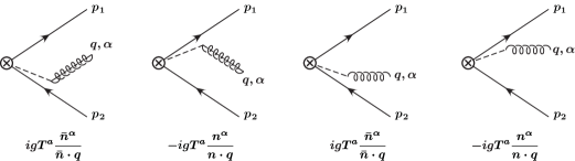
Figure 2: One-gluon Feynman rules for $O_{2}^{(0)}$. The SCET energy-momentum conserving delta function $\delta_{\rm SCET}$ has been omitted but is implied. Springs are soft gluons, springs with lines are collinear gluons, and solid lines are fermions. Lines angled up are $n$-collinear, angled down are $\bar{n}$-collinear, and horizontal are soft. The dashed lines represent the emission from a Wilson line.

The terms in each square bracket of (3.1) each transform under a separate $SU(3)$ symmetry, corresponding to the various sectors of the theory and represents a different decoupled sector giving the physical picture of Fig. 3, which we explain below.

(a) $n$-collinear

(b) soft

(c) $\bar{n}$-collinear

Figure 3: Physical picture of $O_{2}^{(0)}$ as seen in each of the three sectors. The dashed lines represent Wilson lines and the solid lines represent fermions.

It is straightforward to show that the one-gluon matrix element of $O_{2}^{(0)}$ reproduces the QCD amplitude at leading order in $\lambda$. The one-gluon amplitudes in Fig. 1 in QCD are

$$i{\mathcal{M}}_{a}=-igT^{a}\bar{u}(p_{1})\frac{2p_{1}^{\alpha}+\gamma^{\alpha}\mathchoice{\ooalign{$\hfil\displaystyle\mkern 0.0mu/\hfil$\crcr$\displaystyle q$}}{\ooalign{$\hfil\textstyle\mkern 0.0mu/\hfil$\crcr$\textstyle q$}}{\ooalign{$\hfil\scriptstyle\mkern 0.0mu/\hfil$\crcr$\scriptstyle q$}}{\ooalign{$\hfil\scriptscriptstyle\mkern 0.0mu/\hfil$\crcr$\scriptscriptstyle q$}}}{2p_{1}\cdot q}\Gamma v(p_{2})\epsilon^{*}_{\alpha}(q)\delta^{(4)}_{\mbox{\tiny QCD}}(Q;p_{1}+p_{2}+q)$$ (83)

and

$$i{\mathcal{M}}_{b} = igT^{a}\bar{u}(p_{1})\Gamma\frac{2p_{2}^{\alpha}+\mathchoice{\ooalign{$\hfil\displaystyle\mkern 0.0mu/\hfil$\crcr$\displaystyle q$}}{\ooalign{$\hfil\textstyle\mkern 0.0mu/\hfil$\crcr$\textstyle q$}}{\ooalign{$\hfil\scriptstyle\mkern 0.0mu/\hfil$\crcr$\scriptstyle q$}}{\ooalign{$\hfil\scriptscriptstyle\mkern 0.0mu/\hfil$\crcr$\scriptscriptstyle q$}}\gamma^{\alpha}}{2p_{2}\cdot q}v(p_{2})\epsilon^{*}_{\alpha}(q)\delta^{(4)}_{\mbox{\tiny QCD}}(Q;p_{1}+p_{2}+q)$$ (92)

where $\Gamma$ is the Dirac structure of the external current. The corresponding leading order contributions in SCET comes from an $n$-collinear quark, $\bar{n}$-collinear antiquark, and a gluon which is either soft or collinear, each of which gives a different result in SCET.

We first consider the case in which the $n$-collinear quark emits an $n$-collinear gluon. Using the Dirac Equation $\mathchoice{\ooalign{$\hfil\displaystyle\mkern 0.0mu/\hfil$\crcr$\displaystyle p$}}{\ooalign{$\hfil\textstyle\mkern 0.0mu/\hfil$\crcr$\textstyle p$}}{\ooalign{$\hfil\scriptstyle\mkern 0.0mu/\hfil$\crcr$\scriptstyle p$}}{\ooalign{$\hfil\scriptscriptstyle\mkern 0.0mu/\hfil$\crcr$\scriptscriptstyle p$}}_{n}u(p_{n})=0$ to write

$$u(p_{n}) = \left(1+\frac{\mathchoice{\ooalign{$\hfil\displaystyle\mkern 0.0mu/\hfil$\crcr$\displaystyle p$}}{\ooalign{$\hfil\textstyle\mkern 0.0mu/\hfil$\crcr$\textstyle p$}}{\ooalign{$\hfil\scriptstyle\mkern 0.0mu/\hfil$\crcr$\scriptstyle p$}}{\ooalign{$\hfil\scriptscriptstyle\mkern 0.0mu/\hfil$\crcr$\scriptscriptstyle p$}}_{n,\perp}}{{\bar{n}}\cdot p_{n}}\frac{\mathchoice{\ooalign{$\hfil\displaystyle\mkern 0.0mu/\hfil$\crcr$\displaystyle{\bar{n}}$}}{\ooalign{$\hfil\textstyle\mkern 0.0mu/\hfil$\crcr$\textstyle{\bar{n}}$}}{\ooalign{$\hfil\scriptstyle\mkern 0.0mu/\hfil$\crcr$\scriptstyle{\bar{n}}$}}{\ooalign{$\hfil\scriptscriptstyle\mkern 0.0mu/\hfil$\crcr$\scriptscriptstyle{\bar{n}}$}}}{2}\right)P_{n}u(p_{n})$$ (109)

and similarly for $v(p_{\bar{n}})$, it is straightforward to show that

$$\bar{u}(p_{1})\left(2p_{1}^{\alpha}+\gamma^{\alpha}\mathchoice{\ooalign{$\hfil\displaystyle\mkern 0.0mu/\hfil$\crcr$\displaystyle q$}}{\ooalign{$\hfil\textstyle\mkern 0.0mu/\hfil$\crcr$\textstyle q$}}{\ooalign{$\hfil\scriptstyle\mkern 0.0mu/\hfil$\crcr$\scriptstyle q$}}{\ooalign{$\hfil\scriptscriptstyle\mkern 0.0mu/\hfil$\crcr$\scriptscriptstyle q$}}\right)\Gamma v(p_{2})=\bar{u}(p_{1})\left(2p_{1}^{\alpha}+\gamma^{\alpha}\mathchoice{\ooalign{$\hfil\displaystyle\mkern 0.0mu/\hfil$\crcr$\displaystyle q$}}{\ooalign{$\hfil\textstyle\mkern 0.0mu/\hfil$\crcr$\textstyle q$}}{\ooalign{$\hfil\scriptstyle\mkern 0.0mu/\hfil$\crcr$\scriptstyle q$}}{\ooalign{$\hfil\scriptscriptstyle\mkern 0.0mu/\hfil$\crcr$\scriptscriptstyle q$}}\right)P_{\bar{n}}\Gamma P_{\bar{n}}v(p_{2})+O(\lambda)$$ (126)

so we can expand (83) as

$$i{\mathcal{M}}_{an} = -igT^{a}\bar{u}(p_{1})\frac{2p_{1}^{\alpha}+\gamma^{\alpha}\mathchoice{\ooalign{$\hfil\displaystyle\mkern 0.0mu/\hfil$\crcr$\displaystyle q$}}{\ooalign{$\hfil\textstyle\mkern 0.0mu/\hfil$\crcr$\textstyle q$}}{\ooalign{$\hfil\scriptstyle\mkern 0.0mu/\hfil$\crcr$\scriptstyle q$}}{\ooalign{$\hfil\scriptscriptstyle\mkern 0.0mu/\hfil$\crcr$\scriptscriptstyle q$}}}{2p_{1}\cdot q}P_{\bar{n}}\Gamma P_{\bar{n}}v(p_{2})\epsilon^{*}_{\alpha}(q)\delta^{(4)}_{\mbox{\tiny SCET}}(Q;p_{1}+q,p_{2})+O(\lambda).$$ (135)

With the projectors $P_{\bar{n}}$ now surrounding the Dirac structure $\Gamma$, this is precisely the amplitude in the effective theory for a $q$-$\bar{q}$ pair to be produced by $O_{2}^{(0)}$, followed by the emission of an $n$-collinear gluon from the $n$-collinear quark through the usual QCD vertex. It is useful to compare this with the expression for the same graph in label SCET:

$$i{\mathcal{M}}_{an}^{\prime} = -igT^{a}\bar{\xi}_{n,\tilde{p}_{1}}(k_{1})\left(n^{\alpha}+{\gamma^{\alpha}_{\perp}\mathchoice{\ooalign{$\hfil\displaystyle\mkern 0.0mu/\hfil$\crcr$\displaystyle p$}}{\ooalign{$\hfil\textstyle\mkern 0.0mu/\hfil$\crcr$\textstyle p$}}{\ooalign{$\hfil\scriptstyle\mkern 0.0mu/\hfil$\crcr$\scriptstyle p$}}{\ooalign{$\hfil\scriptscriptstyle\mkern 0.0mu/\hfil$\crcr$\scriptscriptstyle p$}}_{1\perp}\over{\bar{n}}\cdot p_{1}}+{(\mathchoice{\ooalign{$\hfil\displaystyle\mkern 0.0mu/\hfil$\crcr$\displaystyle p$}}{\ooalign{$\hfil\textstyle\mkern 0.0mu/\hfil$\crcr$\textstyle p$}}{\ooalign{$\hfil\scriptstyle\mkern 0.0mu/\hfil$\crcr$\scriptstyle p$}}{\ooalign{$\hfil\scriptscriptstyle\mkern 0.0mu/\hfil$\crcr$\scriptscriptstyle p$}}_{1\perp}+\mathchoice{\ooalign{$\hfil\displaystyle\mkern 0.0mu/\hfil$\crcr$\displaystyle q$}}{\ooalign{$\hfil\textstyle\mkern 0.0mu/\hfil$\crcr$\textstyle q$}}{\ooalign{$\hfil\scriptstyle\mkern 0.0mu/\hfil$\crcr$\scriptstyle q$}}{\ooalign{$\hfil\scriptscriptstyle\mkern 0.0mu/\hfil$\crcr$\scriptscriptstyle q$}}_{\perp})\gamma^{\alpha}_{\perp}\over{\bar{n}}\cdot(p_{1}+q)}+{(\mathchoice{\ooalign{$\hfil\displaystyle\mkern 0.0mu/\hfil$\crcr$\displaystyle p$}}{\ooalign{$\hfil\textstyle\mkern 0.0mu/\hfil$\crcr$\textstyle p$}}{\ooalign{$\hfil\scriptstyle\mkern 0.0mu/\hfil$\crcr$\scriptstyle p$}}{\ooalign{$\hfil\scriptscriptstyle\mkern 0.0mu/\hfil$\crcr$\scriptscriptstyle p$}}_{1\perp}+\mathchoice{\ooalign{$\hfil\displaystyle\mkern 0.0mu/\hfil$\crcr$\displaystyle q$}}{\ooalign{$\hfil\textstyle\mkern 0.0mu/\hfil$\crcr$\textstyle q$}}{\ooalign{$\hfil\scriptstyle\mkern 0.0mu/\hfil$\crcr$\scriptstyle q$}}{\ooalign{$\hfil\scriptscriptstyle\mkern 0.0mu/\hfil$\crcr$\scriptscriptstyle q$}}_{\perp})\mathchoice{\ooalign{$\hfil\displaystyle\mkern 0.0mu/\hfil$\crcr$\displaystyle p$}}{\ooalign{$\hfil\textstyle\mkern 0.0mu/\hfil$\crcr$\textstyle p$}}{\ooalign{$\hfil\scriptstyle\mkern 0.0mu/\hfil$\crcr$\scriptstyle p$}}{\ooalign{$\hfil\scriptscriptstyle\mkern 0.0mu/\hfil$\crcr$\scriptscriptstyle p$}}_{1\perp}\over{\bar{n}}\cdot p_{1}\;{\bar{n}}\cdot(p_{1}+q)}{\bar{n}}^{\alpha}\right)\frac{\mathchoice{\ooalign{$\hfil\displaystyle\mkern 0.0mu/\hfil$\crcr$\displaystyle{\bar{n}}$}}{\ooalign{$\hfil\textstyle\mkern 0.0mu/\hfil$\crcr$\textstyle{\bar{n}}$}}{\ooalign{$\hfil\scriptstyle\mkern 0.0mu/\hfil$\crcr$\scriptstyle{\bar{n}}$}}{\ooalign{$\hfil\scriptscriptstyle\mkern 0.0mu/\hfil$\crcr$\scriptscriptstyle{\bar{n}}$}}}{2}$$ (192)

$$\times \left(\frac{\mathchoice{\ooalign{$\hfil\displaystyle\mkern 0.0mu/\hfil$\crcr$\displaystyle n$}}{\ooalign{$\hfil\textstyle\mkern 0.0mu/\hfil$\crcr$\textstyle n$}}{\ooalign{$\hfil\scriptstyle\mkern 0.0mu/\hfil$\crcr$\scriptstyle n$}}{\ooalign{$\hfil\scriptscriptstyle\mkern 0.0mu/\hfil$\crcr$\scriptscriptstyle n$}}}{2}{{\bar{n}}\cdot(p_{1}+q)\over n\cdot(k_{1}+k_{3})\;{\bar{n}}\cdot(p_{1}+q)+(p_{1\perp}+q_{\perp})^{2}}\right)\Gamma\xi_{{\bar{n}},\tilde{p}_{2}}(k_{2})\epsilon^{*}_{n,\tilde{q}\,\alpha}(k_{3})$$ (201)

$$\times \delta_{{\bar{n}}\cdot(\tilde{p}_{1}+\tilde{q}),Q}\delta_{n\cdot\tilde{p}_{2},Q}\delta_{0,\tilde{p}_{1\perp}+\tilde{p}_{2\perp}+\tilde{q}_{\perp}}\delta^{(4)}(k_{1}+k_{2}+k_{3})$$ (202)

where the first factor in parentheses is the collinear quark - collinear quark - collinear gluon vertex, the second is the collinear quark propagator in label SCET, and the $\xi$ fields are two-component spinors. Some straightforward Dirac algebra shows that this is indeed equivalent to the expression (135); however, the more complicated Feynman rules of label SCET, arising from the fact that the collinear spinors are 2-component objects rather than 4-component spinors obeying (109), makes the intermediate expression considerably more complicated.

Expanding the amplitude in which an $n$-collinear gluon is emitted from an $\bar{n}$-collinear antiquark, (92), in powers of $\lambda$ gives

$$i{\mathcal{M}}_{bn}=igT^{a}\frac{{\bar{n}}^{\alpha}}{{\bar{n}}\cdot q}\bar{u}(p_{1})P_{\bar{n}}\Gamma P_{\bar{n}}v(p_{2})\epsilon^{*}_{\alpha}(q)\delta^{(4)}_{\mbox{\tiny SCET}}(Q;p_{1}+q,p_{2})+O(\lambda)$$ (203)

where we have used the expansions

$$2p_{2}\cdot q = (p_{2}\cdot n)(q\cdot{\bar{n}})+O(\lambda^{2})$$

$$2p_{2}\cdot\epsilon^{*}(q) = (p_{2}\cdot n)(\epsilon^{*}(q)\cdot{\bar{n}})+O(\lambda^{2}).$$ (204)

In SCET, the $n$-collinear quark does not couple to the $\bar{n}$-collinear antiquark directly, but rather to the Wilson line $W_{n}^{(\bf 3)}(x_{\bar{n}},x_{\bar{n}}^{\infty})$ in $O_{2}^{(0)}$, and this amplitude is reproduced in the effective theory by the graph in which the Wilson line emits the $n$-collinear quark. The interactions (135) and (203) of the $n$-collinear gluon is represented in Fig. 3(a) by a QCD quark field in the $n$ direction and a Wilson line in the ${\bar{n}}$ direction.

Similarly, the amplitudes in Fig. 1 are reproduced for $\bar{n}$-collinear gluons in SCET by a gluon emitted from a semi-infinite $n$-collinear Wilson line $W_{\bar{n}}^{(\bf 3)}(x_{n},x_{n}^{\infty})$, and the usual QCD Feynman rules for gluon emission, respectively. The $\bar{n}$-collinear gluon interaction is represented in Fig. 3(c).

Finally, the amplitude for soft gluon emission from the quark and antiquark lines is obtained by expanding the sum of the two previous graphs for soft gluon momentum,

$$i{\mathcal{M}}_{s}=-igT^{a}\left(\frac{n^{\alpha}}{n\cdot q}-\frac{{\bar{n}}^{\alpha}}{{\bar{n}}\cdot q}\right)\bar{u}(p_{1})P_{n}\Gamma P_{\bar{n}}v(p_{2})\epsilon^{*}_{\alpha}(q)\delta^{(4)}_{\mbox{\tiny SCET}}(Q;p_{1},p_{2})+O(\lambda),$$ (205)

which is the amplitude for gluon emission from a fundamental and anti-fundamental Wilson line, $Y_{n}^{(\bf 3)}(x_{n}^{\infty_{s}},0)$ and $Y_{\bar{n}}^{(\bf 3)}(0,x_{{\bar{n}}}^{\infty_{s}})$ respectively, represented in Fig. 3(b).

Thus, we have shown that $O_{2}^{(0)}$ as defined in (3.1) reproduces the leading order QCD $q\bar{q}g$ production amplitudes. In the next section, we will show how $O(\lambda)$ operators arise as generalizations of $O_{2}^{(0)}$ and the physical picture of Fig. 3.

3.2 Subleading Corrections to Dijet Production

At leading order, the external current is written as a product of QCD fields coupled to Wilson lines. Higher order corrections to the current are therefore expected to have the same structure, but with insertions of derivatives and additional fields, in the same way that subleading twist shape functions and parton distributions are related to the leading order operators [11, 12]. Defining the external current to subleading order in (34) where the $O_{2}^{(1i)}$’s are $O(\lambda)$, it is straightforward to determine the required operators $O_{2}^{(1i)}$ and coefficient functions $C_{2}^{(1i)}$ by carrying out the expansion of the previous section to higher orders in $\lambda$. Starting with the emission of an $n$-collinear gluon, we can expand the QCD amplitudes (83) and (92) to $O(\lambda)$:

$$i{\mathcal{M}}_{(a,b)n}=-igT^{a}\bar{u}(p_{1})\Gamma^{\alpha}_{(a,b)n}v(p_{2})\epsilon^{*}_{\alpha}(q)\delta^{(4)}_{\mbox{\tiny SCET}}(Q;p_{1}+q,p_{2})+O(\lambda^{2})$$ (206)

where

$$\Gamma^{\alpha}_{an} = {\left(2p_{1}^{\alpha}+\gamma^{\alpha}\mathchoice{\ooalign{$\hfil\displaystyle\mkern 0.0mu/\hfil$\crcr$\displaystyle q$}}{\ooalign{$\hfil\textstyle\mkern 0.0mu/\hfil$\crcr$\textstyle q$}}{\ooalign{$\hfil\scriptstyle\mkern 0.0mu/\hfil$\crcr$\scriptstyle q$}}{\ooalign{$\hfil\scriptscriptstyle\mkern 0.0mu/\hfil$\crcr$\scriptscriptstyle q$}}\right)\over 2p_{1}\cdot q}P_{\bar{n}}\Gamma P_{\bar{n}}-{\Delta^{\alpha\mu}(\bar{n},p_{1})\over{\bar{n}}\cdot(p_{1}+q)}\frac{\mathchoice{\ooalign{$\hfil\displaystyle\mkern 0.0mu/\hfil$\crcr$\displaystyle\bar{n}$}}{\ooalign{$\hfil\textstyle\mkern 0.0mu/\hfil$\crcr$\textstyle\bar{n}$}}{\ooalign{$\hfil\scriptstyle\mkern 0.0mu/\hfil$\crcr$\scriptstyle\bar{n}$}}{\ooalign{$\hfil\scriptscriptstyle\mkern 0.0mu/\hfil$\crcr$\scriptscriptstyle\bar{n}$}}}{2}\gamma_{\mu\perp}\Gamma P_{\bar{n}}+{\left(2p_{1}^{\alpha}+\gamma^{\alpha}\mathchoice{\ooalign{$\hfil\displaystyle\mkern 0.0mu/\hfil$\crcr$\displaystyle q$}}{\ooalign{$\hfil\textstyle\mkern 0.0mu/\hfil$\crcr$\textstyle q$}}{\ooalign{$\hfil\scriptstyle\mkern 0.0mu/\hfil$\crcr$\scriptstyle q$}}{\ooalign{$\hfil\scriptscriptstyle\mkern 0.0mu/\hfil$\crcr$\scriptscriptstyle q$}}\right)\over 2p_{1}\cdot q}{\mathchoice{\ooalign{$\hfil\displaystyle\mkern 0.0mu/\hfil$\crcr$\displaystyle\bar{n}$}}{\ooalign{$\hfil\textstyle\mkern 0.0mu/\hfil$\crcr$\textstyle\bar{n}$}}{\ooalign{$\hfil\scriptstyle\mkern 0.0mu/\hfil$\crcr$\scriptstyle\bar{n}$}}{\ooalign{$\hfil\scriptscriptstyle\mkern 0.0mu/\hfil$\crcr$\scriptscriptstyle\bar{n}$}}\over 2}{\left(\mathchoice{\ooalign{$\hfil\displaystyle\mkern 0.0mu/\hfil$\crcr$\displaystyle p$}}{\ooalign{$\hfil\textstyle\mkern 0.0mu/\hfil$\crcr$\textstyle p$}}{\ooalign{$\hfil\scriptstyle\mkern 0.0mu/\hfil$\crcr$\scriptstyle p$}}{\ooalign{$\hfil\scriptscriptstyle\mkern 0.0mu/\hfil$\crcr$\scriptscriptstyle p$}}_{1\perp}+\mathchoice{\ooalign{$\hfil\displaystyle\mkern 0.0mu/\hfil$\crcr$\displaystyle q$}}{\ooalign{$\hfil\textstyle\mkern 0.0mu/\hfil$\crcr$\textstyle q$}}{\ooalign{$\hfil\scriptstyle\mkern 0.0mu/\hfil$\crcr$\scriptstyle q$}}{\ooalign{$\hfil\scriptscriptstyle\mkern 0.0mu/\hfil$\crcr$\scriptscriptstyle q$}}\right)\over\bar{n}\cdot\left(p_{1}+q\right)}\Gamma P_{\bar{n}}$$ (255)

and

$$\Gamma^{\alpha}_{bn} = -\frac{{\bar{n}}^{\alpha}}{{\bar{n}}\cdot q}P_{\bar{n}}\Gamma P_{\bar{n}}-\frac{{\bar{n}}^{\alpha}}{{\bar{n}}\cdot q}\frac{\mathchoice{\ooalign{$\hfil\displaystyle\mkern 0.0mu/\hfil$\crcr$\displaystyle{\bar{n}}$}}{\ooalign{$\hfil\textstyle\mkern 0.0mu/\hfil$\crcr$\textstyle{\bar{n}}$}}{\ooalign{$\hfil\scriptstyle\mkern 0.0mu/\hfil$\crcr$\scriptstyle{\bar{n}}$}}{\ooalign{$\hfil\scriptscriptstyle\mkern 0.0mu/\hfil$\crcr$\scriptscriptstyle{\bar{n}}$}}}{2}\frac{\mathchoice{\ooalign{$\hfil\displaystyle\mkern 0.0mu/\hfil$\crcr$\displaystyle p$}}{\ooalign{$\hfil\textstyle\mkern 0.0mu/\hfil$\crcr$\textstyle p$}}{\ooalign{$\hfil\scriptstyle\mkern 0.0mu/\hfil$\crcr$\scriptstyle p$}}{\ooalign{$\hfil\scriptscriptstyle\mkern 0.0mu/\hfil$\crcr$\scriptscriptstyle p$}}_{1\perp}}{{\bar{n}}\cdot p_{1}}\Gamma P_{\bar{n}}+\frac{1}{Q}\Delta^{\alpha\mu}({\bar{n}},q)P_{\bar{n}}\Gamma\mbox{$\gamma_{\mu}$}_{\perp}\frac{\mathchoice{\ooalign{$\hfil\displaystyle\mkern 0.0mu/\hfil$\crcr$\displaystyle n$}}{\ooalign{$\hfil\textstyle\mkern 0.0mu/\hfil$\crcr$\textstyle n$}}{\ooalign{$\hfil\scriptstyle\mkern 0.0mu/\hfil$\crcr$\scriptstyle n$}}{\ooalign{$\hfil\scriptscriptstyle\mkern 0.0mu/\hfil$\crcr$\scriptscriptstyle n$}}}{2}$$ (281)

where we have defined

$$\Delta^{\alpha\mu}(\bar{n},p)=g^{\alpha\mu}-\frac{\bar{n}^{\alpha}p^{\mu}}{\bar{n}\cdot p}$$ (282)

and we have used the expansion

$$\mathchoice{\ooalign{$\hfil\displaystyle\mkern 0.0mu/\hfil$\crcr$\displaystyle q$}}{\ooalign{$\hfil\textstyle\mkern 0.0mu/\hfil$\crcr$\textstyle q$}}{\ooalign{$\hfil\scriptstyle\mkern 0.0mu/\hfil$\crcr$\scriptstyle q$}}{\ooalign{$\hfil\scriptscriptstyle\mkern 0.0mu/\hfil$\crcr$\scriptscriptstyle q$}}\mathchoice{\ooalign{$\hfil\displaystyle\mkern 0.0mu/\hfil$\crcr$\displaystyle\epsilon$}}{\ooalign{$\hfil\textstyle\mkern 0.0mu/\hfil$\crcr$\textstyle\epsilon$}}{\ooalign{$\hfil\scriptstyle\mkern 0.0mu/\hfil$\crcr$\scriptstyle\epsilon$}}{\ooalign{$\hfil\scriptscriptstyle\mkern 0.0mu/\hfil$\crcr$\scriptscriptstyle\epsilon$}}^{*}(q)=({\bar{n}}\cdot q)\frac{\mathchoice{\ooalign{$\hfil\displaystyle\mkern 0.0mu/\hfil$\crcr$\displaystyle n$}}{\ooalign{$\hfil\textstyle\mkern 0.0mu/\hfil$\crcr$\textstyle n$}}{\ooalign{$\hfil\scriptstyle\mkern 0.0mu/\hfil$\crcr$\scriptstyle n$}}{\ooalign{$\hfil\scriptscriptstyle\mkern 0.0mu/\hfil$\crcr$\scriptscriptstyle n$}}}{2}\mbox{$\gamma_{\mu}$}_{\perp}\Delta^{\alpha\mu}({\bar{n}},q)\epsilon^{*}_{\alpha}(q)+O(\lambda^{2})$$ (283)

as well as the spinor expansion (109). The sum of the graphs is

$$\Gamma^{\alpha}_{an}+\Gamma^{\alpha}_{bn} = {\left(2p_{1}^{\alpha}+\gamma^{\alpha}\mathchoice{\ooalign{$\hfil\displaystyle\mkern 0.0mu/\hfil$\crcr$\displaystyle q$}}{\ooalign{$\hfil\textstyle\mkern 0.0mu/\hfil$\crcr$\textstyle q$}}{\ooalign{$\hfil\scriptstyle\mkern 0.0mu/\hfil$\crcr$\scriptstyle q$}}{\ooalign{$\hfil\scriptscriptstyle\mkern 0.0mu/\hfil$\crcr$\scriptscriptstyle q$}}\right)\over 2p_{1}\cdot q}P_{\bar{n}}\Gamma P_{\bar{n}}-\frac{{\bar{n}}^{\alpha}}{{\bar{n}}\cdot q}P_{\bar{n}}\Gamma P_{\bar{n}}$$ (292)

$$+ \frac{1}{Q}\left[\Delta^{\alpha\mu}({\bar{n}},q)P_{\bar{n}}\Gamma\mbox{$\gamma_{\mu}$}_{\perp}\frac{\mathchoice{\ooalign{$\hfil\displaystyle\mkern 0.0mu/\hfil$\crcr$\displaystyle n$}}{\ooalign{$\hfil\textstyle\mkern 0.0mu/\hfil$\crcr$\textstyle n$}}{\ooalign{$\hfil\scriptstyle\mkern 0.0mu/\hfil$\crcr$\scriptstyle n$}}{\ooalign{$\hfil\scriptscriptstyle\mkern 0.0mu/\hfil$\crcr$\scriptscriptstyle n$}}}{2}+\frac{\mathchoice{\ooalign{$\hfil\displaystyle\mkern 0.0mu/\hfil$\crcr$\displaystyle{\bar{n}}$}}{\ooalign{$\hfil\textstyle\mkern 0.0mu/\hfil$\crcr$\textstyle{\bar{n}}$}}{\ooalign{$\hfil\scriptstyle\mkern 0.0mu/\hfil$\crcr$\scriptstyle{\bar{n}}$}}{\ooalign{$\hfil\scriptscriptstyle\mkern 0.0mu/\hfil$\crcr$\scriptscriptstyle{\bar{n}}$}}}{2}\left(\gamma^{\alpha}_{\perp}+\frac{{\bar{n}}^{\alpha}}{{\bar{n}}\cdot q}\mathchoice{\ooalign{$\hfil\displaystyle\mkern 0.0mu/\hfil$\crcr$\displaystyle p$}}{\ooalign{$\hfil\textstyle\mkern 0.0mu/\hfil$\crcr$\textstyle p$}}{\ooalign{$\hfil\scriptstyle\mkern 0.0mu/\hfil$\crcr$\scriptstyle p$}}{\ooalign{$\hfil\scriptscriptstyle\mkern 0.0mu/\hfil$\crcr$\scriptscriptstyle p$}}_{1\perp}\right)\Gamma P_{\bar{n}}\right.$$ (317)

$$+ \left.{\left(2p_{1}^{\alpha}+\gamma^{\alpha}\mathchoice{\ooalign{$\hfil\displaystyle\mkern 0.0mu/\hfil$\crcr$\displaystyle q$}}{\ooalign{$\hfil\textstyle\mkern 0.0mu/\hfil$\crcr$\textstyle q$}}{\ooalign{$\hfil\scriptstyle\mkern 0.0mu/\hfil$\crcr$\scriptstyle q$}}{\ooalign{$\hfil\scriptscriptstyle\mkern 0.0mu/\hfil$\crcr$\scriptscriptstyle q$}}\right)\over 2p_{1}\cdot q}{\mathchoice{\ooalign{$\hfil\displaystyle\mkern 0.0mu/\hfil$\crcr$\displaystyle\bar{n}$}}{\ooalign{$\hfil\textstyle\mkern 0.0mu/\hfil$\crcr$\textstyle\bar{n}$}}{\ooalign{$\hfil\scriptstyle\mkern 0.0mu/\hfil$\crcr$\scriptstyle\bar{n}$}}{\ooalign{$\hfil\scriptscriptstyle\mkern 0.0mu/\hfil$\crcr$\scriptscriptstyle\bar{n}$}}\over 2}\left(\mathchoice{\ooalign{$\hfil\displaystyle\mkern 0.0mu/\hfil$\crcr$\displaystyle p$}}{\ooalign{$\hfil\textstyle\mkern 0.0mu/\hfil$\crcr$\textstyle p$}}{\ooalign{$\hfil\scriptstyle\mkern 0.0mu/\hfil$\crcr$\scriptstyle p$}}{\ooalign{$\hfil\scriptscriptstyle\mkern 0.0mu/\hfil$\crcr$\scriptscriptstyle p$}}_{1\perp}+\mathchoice{\ooalign{$\hfil\displaystyle\mkern 0.0mu/\hfil$\crcr$\displaystyle q$}}{\ooalign{$\hfil\textstyle\mkern 0.0mu/\hfil$\crcr$\textstyle q$}}{\ooalign{$\hfil\scriptstyle\mkern 0.0mu/\hfil$\crcr$\scriptstyle q$}}{\ooalign{$\hfil\scriptscriptstyle\mkern 0.0mu/\hfil$\crcr$\scriptscriptstyle q$}}\right)\Gamma P_{\bar{n}}\right].$$ (350)

The first two terms of (292) are $O(1)$, while the remaining terms are $O(\lambda)$, and are reproduced in the effective theory by the operators

$$O^{(1a_{n})}_{2} = \left[\bar{\psi}_{n}(x_{\bar{n}})P_{\bar{n}}\Gamma i\mathchoice{\ooalign{$\hfil\displaystyle\mkern 0.0mu/\hfil$\crcr$\displaystyle D$}}{\ooalign{$\hfil\textstyle\mkern 0.0mu/\hfil$\crcr$\textstyle D$}}{\ooalign{$\hfil\scriptstyle\mkern 0.0mu/\hfil$\crcr$\scriptstyle D$}}{\ooalign{$\hfil\scriptscriptstyle\mkern 0.0mu/\hfil$\crcr$\scriptscriptstyle D$}}_{\perp}(x_{\bar{n}})W_{n}^{(\bf 3)}(x_{\bar{n}},x_{\bar{n}}^{\infty})\right]\left[Y_{n}^{(\bf 3)}(x_{n}^{\infty_{s}},0)Y_{\bar{n}}^{(\bf 3)}(0,x_{{\bar{n}}}^{\infty_{s}})\right]$$ (368)

$$\qquad\times\left[W_{\bar{n}}^{(\bf 3)}(x_{n}^{\infty},x_{n})\frac{\mathchoice{\ooalign{$\hfil\displaystyle\mkern 0.0mu/\hfil$\crcr$\displaystyle n$}}{\ooalign{$\hfil\textstyle\mkern 0.0mu/\hfil$\crcr$\textstyle n$}}{\ooalign{$\hfil\scriptstyle\mkern 0.0mu/\hfil$\crcr$\scriptstyle n$}}{\ooalign{$\hfil\scriptscriptstyle\mkern 0.0mu/\hfil$\crcr$\scriptscriptstyle n$}}}{2}\psi_{\bar{n}}(x_{n})\right]$$

$$O_{2}^{(1b_{n})} = \left[\bar{\psi}_{n}(x_{\bar{n}})\frac{\mathchoice{\ooalign{$\hfil\displaystyle\mkern 0.0mu/\hfil$\crcr$\displaystyle{\bar{n}}$}}{\ooalign{$\hfil\textstyle\mkern 0.0mu/\hfil$\crcr$\textstyle{\bar{n}}$}}{\ooalign{$\hfil\scriptstyle\mkern 0.0mu/\hfil$\crcr$\scriptstyle{\bar{n}}$}}{\ooalign{$\hfil\scriptscriptstyle\mkern 0.0mu/\hfil$\crcr$\scriptscriptstyle{\bar{n}}$}}}{2}i\overleftarrow{\mathchoice{\ooalign{$\hfil\displaystyle\mkern 0.0mu/\hfil$\crcr$\displaystyle D$}}{\ooalign{$\hfil\textstyle\mkern 0.0mu/\hfil$\crcr$\textstyle D$}}{\ooalign{$\hfil\scriptstyle\mkern 0.0mu/\hfil$\crcr$\scriptstyle D$}}{\ooalign{$\hfil\scriptscriptstyle\mkern 0.0mu/\hfil$\crcr$\scriptscriptstyle D$}}}_{\perp}(x_{\bar{n}})\Gamma W_{n}^{(\bf 3)}(x_{\bar{n}},x_{\bar{n}}^{\infty})\right]\left[Y_{n}^{(\bf 3)}(x_{n}^{\infty_{s}},0)Y_{\bar{n}}^{(\bf 3)}(0,x_{{\bar{n}}}^{\infty_{s}})\right]$$ (386)

$$\qquad\times\left[W_{\bar{n}}^{(\bf 3)}(x_{n}^{\infty},x_{n})P_{\bar{n}}\psi_{\bar{n}}(x_{n})\right]$$

where the covariant derivatives are defined in the usual way

$$D^{\mu}\psi_{n,{\bar{n}},s}=\partial^{\mu}\psi_{n,{\bar{n}},s}-igT^{a}A^{\mu a}_{n,{\bar{n}},s}\psi_{n,{\bar{n}},s}$$ (387)

to only couple the corresponding gluon fields to $n$-collinear, $\bar{n}$-collinear, and soft quarks, respectively. The one-gluon Feynman rules for these operators are given in Fig. 6. The last term in (292) corresponds in the effective theory to a gluon emitted from the $n$-collinear quark leg via ${\cal L}_{\rm QCD}$ after the insertion of the subleading operator $O_{2}^{(1b_{n})}$. From (292), we find $C_{2}^{(1a_{n})}=-1+O(\alpha_{s})$ and $C_{2}^{(1b_{n})}=1+O(\alpha_{s})$.

We can perform a similar expansion for soft gluon emission. Expanding the amplitude (83) for soft momentum $q^{\mu}$, including the multipole expansion (38), gives

$$i{\mathcal{M}}_{as} = -igT^{a}\left[\bar{u}(p_{1})P_{\bar{n}}\Gamma P_{\bar{n}}v(p_{2})\left({n^{\alpha}\over n\cdot q}\left(1+q^{\mu}_{\perp}{\partial\over\partial p_{1\perp}^{\mu}}\right)\right.+\frac{2p_{1\perp\mu}}{Q\;n\cdot q}\Delta^{\alpha\mu}(n,q)\right)$$ (388)

$$+ \left.{n^{\alpha}\over 2Q\;n\cdot q}\bar{u}(p_{1})\left(\mathchoice{\ooalign{$\hfil\displaystyle\mkern 0.0mu/\hfil$\crcr$\displaystyle{\bar{n}}$}}{\ooalign{$\hfil\textstyle\mkern 0.0mu/\hfil$\crcr$\textstyle{\bar{n}}$}}{\ooalign{$\hfil\scriptstyle\mkern 0.0mu/\hfil$\crcr$\scriptstyle{\bar{n}}$}}{\ooalign{$\hfil\scriptscriptstyle\mkern 0.0mu/\hfil$\crcr$\scriptscriptstyle{\bar{n}}$}}\mathchoice{\ooalign{$\hfil\displaystyle\mkern 0.0mu/\hfil$\crcr$\displaystyle p$}}{\ooalign{$\hfil\textstyle\mkern 0.0mu/\hfil$\crcr$\textstyle p$}}{\ooalign{$\hfil\scriptstyle\mkern 0.0mu/\hfil$\crcr$\scriptstyle p$}}{\ooalign{$\hfil\scriptscriptstyle\mkern 0.0mu/\hfil$\crcr$\scriptscriptstyle p$}}_{1\perp}\Gamma P_{\bar{n}}+P_{\bar{n}}\Gamma\mathchoice{\ooalign{$\hfil\displaystyle\mkern 0.0mu/\hfil$\crcr$\displaystyle p$}}{\ooalign{$\hfil\textstyle\mkern 0.0mu/\hfil$\crcr$\textstyle p$}}{\ooalign{$\hfil\scriptstyle\mkern 0.0mu/\hfil$\crcr$\scriptstyle p$}}{\ooalign{$\hfil\scriptscriptstyle\mkern 0.0mu/\hfil$\crcr$\scriptscriptstyle p$}}_{2\perp}\mathchoice{\ooalign{$\hfil\displaystyle\mkern 0.0mu/\hfil$\crcr$\displaystyle n$}}{\ooalign{$\hfil\textstyle\mkern 0.0mu/\hfil$\crcr$\textstyle n$}}{\ooalign{$\hfil\scriptstyle\mkern 0.0mu/\hfil$\crcr$\scriptstyle n$}}{\ooalign{$\hfil\scriptscriptstyle\mkern 0.0mu/\hfil$\crcr$\scriptscriptstyle n$}}\right)v(p_{2})\right]\epsilon^{*}_{\alpha}(q)\delta^{(4)}_{\mbox{\tiny SCET}}(Q;p_{1},p_{2})+O(\lambda^{2}).$$ (421)

The second line in (388) is reproduced in the effective theory by $O_{2}^{(1b_{n})}$, followed by emission of a soft gluon off the soft Wilson line $Y_{n}$, and so has already been accounted for. The term proportional to $\Delta^{\alpha\mu}(n,q)$ requires the introduction of the operator

$$O_{2}^{(1c_{ns})}(x) = -i\int_{0}^{\infty}dt\left[\bar{\psi}_{n}(x_{\bar{n}})P_{\bar{n}}\Gamma i\overleftarrow{D}^{\mu}_{\perp}W_{n}^{(\bf 3)}(x_{\bar{n}},x_{\bar{n}}^{\infty})\right]$$

$$\times \left[Y_{n}^{(\bf 3)}(x_{n}^{\infty_{s}},tn)i\overleftarrow{D}_{\perp\mu}(tn)Y_{n}^{(\bf 3)}(tn,0)Y_{\bar{n}}^{(\bf 3)}(0,x_{{\bar{n}}}^{\infty_{s}})\right]\left[W_{\bar{n}}^{(\bf 3)}(x_{n}^{\infty},x_{n})P_{\bar{n}}\psi_{\bar{n}}(x_{n})\right]$$

while the higher order term in the multipole expansion of the momentum requires the operator

$$O^{(1\delta_{s})}_{2}(x) = Q\left[\bar{\psi}_{n}(x_{\bar{n}})P_{\bar{n}}\Gamma W_{n}^{(\bf 3)}(x_{\bar{n}},x_{\bar{n}}^{\infty})\right]\left[Y_{n}^{(\bf 3)}(x_{n}^{\infty_{s}},0)(x_{\perp\mu}D_{\perp}^{\mu}+\overleftarrow{D}_{\perp}^{\mu}x_{\perp\mu})Y_{\bar{n}}^{(\bf 3)}(0,x_{{\bar{n}}}^{\infty_{s}})\right]$$ (423)

$$\times \left[W_{\bar{n}}^{(\bf 3)}(x_{n}^{\infty},x_{n})P_{\bar{n}}\psi_{\bar{n}}(x_{n})\right].$$

From (388) we find $C_{2}^{(1c_{ns})}=-2+O(\alpha_{s})$ and $C_{2}^{(1\delta_{s})}=1+O(\alpha_{s})$.

In addition to subleading corrections to the leading order amplitudes, at subleading order additional processes – soft quark and $n$-collinear antiquark emission – occur. In the standard SCET approach, these arise from subleading terms in the effective Lagrangian which directly couple the various sectors. In our formulation, the only coupling between the different sectors occurs via the external current ${\cal J}_{2}^{\rm SCET}$, so these processes are also described in SCET by subleading operators $O_{2}^{(1i)}$.

Consider Fig. 1(a) where the gluon is $n$-collinear and the quark is soft. Expanding the amplitude (83) for these kinematics gives

$$i{\mathcal{M}}_{as_{q}} = -igT^{a}\bar{u}_{s}(p_{1})\frac{\Delta^{\alpha\mu}({\bar{n}},q)}{n\cdot p_{1}}\frac{\mathchoice{\ooalign{$\hfil\displaystyle\mkern 0.0mu/\hfil$\crcr$\displaystyle n$}}{\ooalign{$\hfil\textstyle\mkern 0.0mu/\hfil$\crcr$\textstyle n$}}{\ooalign{$\hfil\scriptstyle\mkern 0.0mu/\hfil$\crcr$\scriptstyle n$}}{\ooalign{$\hfil\scriptscriptstyle\mkern 0.0mu/\hfil$\crcr$\scriptscriptstyle n$}}}{2}\mbox{$\gamma_{\mu}$}_{\perp}\Gamma P_{\bar{n}}v(p_{2})\epsilon^{*}_{\alpha}(q)\delta^{(4)}_{\mbox{\tiny SCET}}(Q;q,p_{2})+O(\lambda^{2}).$$ (432)

The amplitude is reproduced in SCET by the subleading operator

$${O}^{(1d_{ns})}_{2}(x)=-i\int_{0}^{\infty}dt\left[{\bar{n}}_{\mu}igG_{n}^{a\mu\nu}(x_{\bar{n}})W_{n}^{(\bf 8)}{}^{ab}(x_{\bar{n}},x_{\bar{n}}^{\infty})\right]$$

$$\times\left[Y_{n}^{(\bf 8)}{}^{bc}(x_{n}^{\infty_{s}},tn)\bar{\psi}_{s}(tn)Y_{n}^{(\bf 3)}(tn,0)T^{c}\frac{\mathchoice{\ooalign{$\hfil\displaystyle\mkern 0.0mu/\hfil$\crcr$\displaystyle n$}}{\ooalign{$\hfil\textstyle\mkern 0.0mu/\hfil$\crcr$\textstyle n$}}{\ooalign{$\hfil\scriptstyle\mkern 0.0mu/\hfil$\crcr$\scriptstyle n$}}{\ooalign{$\hfil\scriptscriptstyle\mkern 0.0mu/\hfil$\crcr$\scriptscriptstyle n$}}}{2}\mbox{$\gamma_{\nu}$}_{\perp}\Gamma Y_{\bar{n}}^{(\bf 3)}(0,x_{{\bar{n}}}^{\infty_{s}})\right]$$ (441)

$$\times\left[W_{\bar{n}}^{(\bf 3)}(x_{n}^{\infty},x_{n})P_{\bar{n}}\psi_{\bar{n}}(x_{n})\right].$$ (442)

The structure of (3.2) can be understood by generalizing the arguments that led to (3.1). The physical picture of (3.2) is shown in Fig. 4. The $n$-collinear gluon recoiling against the soft quark and $\bar{n}$-collinear antiquark in an $SU(3)$ adjoint looks like a gluon coupled to an adjoint Wilson line, giving the first factor in (3.2) and the picture Fig. 4(a). The $\bar{n}$-collinear sector sees no difference between an antiquark recoiling against an $n$-collinear quark and recoiling against an $n$-collinear gluon and a soft quark in a relative fundamental state, so the third factor is unchanged from (3.1) and gives the picture Fig. 4(c). Finally, the soft sector has fundamental and anti-fundamental Wilson lines emitted by the current as usual, but then the fundamental emits a soft quark and becomes an adjoint Wilson line (the $n$-collinear gluon) as pictured in Fig. 4(b). From (432) we find $C_{2}^{(1d_{ns})}=1+O(\alpha_{s})$.

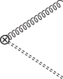
(a) $n$-collinear

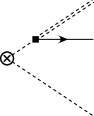
(b) soft

(c) $\bar{n}$-collinear

Figure 4: $O_{2}^{(1d_{ns})}$ as seen in each of the three sectors. The single and double dashed lines represent fundamental and adjoint Wilson lines respectively.

The situation is similar for emission of an $\bar{n}$-collinear gluon recoiling against an $n$-collinear quark-antiquark pair. Expanding the amplitudes (83) and (92), we find the leading order terms cancel between the two diagrams, giving the amplitude

$$i{\mathcal{M}}_{nn\bar{n}} = igT^{a}\epsilon^{*}_{\alpha}(q)\bar{u}(p_{1})\left({{\mathchoice{\ooalign{$\hfil\displaystyle\mkern 0.0mu/\hfil$\crcr$\displaystyle\bar{n}$}}{\ooalign{$\hfil\textstyle\mkern 0.0mu/\hfil$\crcr$\textstyle\bar{n}$}}{\ooalign{$\hfil\scriptstyle\mkern 0.0mu/\hfil$\crcr$\scriptstyle\bar{n}$}}{\ooalign{$\hfil\scriptscriptstyle\mkern 0.0mu/\hfil$\crcr$\scriptscriptstyle\bar{n}$}}\over 2}\gamma_{\mu\perp}\Gamma P_{n}\over{\bar{n}}\cdot p_{1}}-{P_{\bar{n}}\Gamma\gamma_{\mu\perp}{\mathchoice{\ooalign{$\hfil\displaystyle\mkern 0.0mu/\hfil$\crcr$\displaystyle\bar{n}$}}{\ooalign{$\hfil\textstyle\mkern 0.0mu/\hfil$\crcr$\textstyle\bar{n}$}}{\ooalign{$\hfil\scriptstyle\mkern 0.0mu/\hfil$\crcr$\scriptstyle\bar{n}$}}{\ooalign{$\hfil\scriptscriptstyle\mkern 0.0mu/\hfil$\crcr$\scriptscriptstyle\bar{n}$}}\over 2}\over{\bar{n}}\cdot p_{2}}\right)v(p_{2})\Delta^{\mu\alpha}(n,q)\delta^{(4)}_{\mbox{\tiny SCET}}(Q;p_{1}+p_{2},q)$$ (460)

$$\qquad+O(\lambda^{2})$$

These terms are reproduced in SCET by the operators

$$O^{(1e_{nn\bar{n}})}_{2}(x) = -i\int_{0}^{\infty}dt\left[\bar{\psi}_{n}(x_{\bar{n}}+t{\bar{n}})T^{d}\frac{\mathchoice{\ooalign{$\hfil\displaystyle\mkern 0.0mu/\hfil$\crcr$\displaystyle{\bar{n}}$}}{\ooalign{$\hfil\textstyle\mkern 0.0mu/\hfil$\crcr$\textstyle{\bar{n}}$}}{\ooalign{$\hfil\scriptstyle\mkern 0.0mu/\hfil$\crcr$\scriptstyle{\bar{n}}$}}{\ooalign{$\hfil\scriptscriptstyle\mkern 0.0mu/\hfil$\crcr$\scriptscriptstyle{\bar{n}}$}}}{2}\mbox{$\gamma_{\nu}$}_{\perp}\Gamma W_{n}^{(\bf 3)}(x_{\bar{n}}+t{\bar{n}},x_{\bar{n}})P_{n}\psi_{n}(x_{\bar{n}})W_{n}^{(\bf 8)}{}^{dc}(x_{\bar{n}}+t{\bar{n}},x_{\bar{n}}^{\infty})\right]$$ (469)

$$\times \left[Y_{n}^{(\bf 8)}{}^{c\hat{b}}(x_{n}^{\infty_{s}},0)Y_{\bar{n}}^{(\bf 8)}{}^{\hat{b}b}(0,x_{n}^{\infty_{s}})\right]\left[n_{\mu}W_{\bar{n}}^{(\bf 8)}{}^{ba}(x_{n}^{\infty},x_{n})igG_{\bar{n}}^{a\mu\nu}(x_{n})\right]$$ (470)

and

$$O^{(1f_{nn\bar{n}})}_{2}(x) = -i\int_{0}^{\infty}dt\left[\bar{\psi}_{n}(x_{\bar{n}})P_{\bar{n}}\Gamma\mbox{$\gamma_{\nu}$}_{\perp}\frac{\mathchoice{\ooalign{$\hfil\displaystyle\mkern 0.0mu/\hfil$\crcr$\displaystyle{\bar{n}}$}}{\ooalign{$\hfil\textstyle\mkern 0.0mu/\hfil$\crcr$\textstyle{\bar{n}}$}}{\ooalign{$\hfil\scriptstyle\mkern 0.0mu/\hfil$\crcr$\scriptstyle{\bar{n}}$}}{\ooalign{$\hfil\scriptscriptstyle\mkern 0.0mu/\hfil$\crcr$\scriptscriptstyle{\bar{n}}$}}}{2}W_{n}^{(\bf 3)}(x_{\bar{n}},x_{\bar{n}}+t{\bar{n}})T^{d}\psi_{n}(x_{\bar{n}}+t{\bar{n}})W_{n}^{(\bf 8)}{}^{dc}(x_{\bar{n}}+t{\bar{n}},x_{\bar{n}}^{\infty})\right]$$ (479)

$$\times \left[Y_{n}^{(\bf 8)}{}^{c\hat{b}}(x_{n}^{\infty_{s}},0)Y_{\bar{n}}^{(\bf 8)}{}^{\hat{b}b}(0,x_{n}^{\infty_{s}})\right]\left[n_{\mu}W_{\bar{n}}^{(\bf 8)}{}^{ba}(x_{n}^{\infty},x_{n})igG_{\bar{n}}^{a\mu\nu}(x_{n})\right].$$ (480)

$O_{2}^{(1f_{nn\bar{n}})}$ is illustrated in the three frames in Fig. 5. From (460) we find $C_{2}^{(1e_{nn{\bar{n}}})}=-C_{2}^{(1f_{nn{\bar{n}}})}=-1+O(\alpha_{s})$.

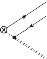
(a) $n$-collinear

(b) soft

(c) $\bar{n}$-collinear

Figure 5: $O_{2}^{(1f_{nn\bar{n}})}$ as seen in each of the three sectors.

Figure 6: One-gluon Feynman rules for NLO dijet operators $O_{2}^{(1i)}$. The notation is the same as Fig. 2. The rule for $O_{2}^{(1b_{n})}$ has been split into two diagrams, depending on whether the gluon is emitted from the vertex or the Wilson line.

There are an additional four operators, defined analogously to the above operators, that arise due to corresponding corrections to the ${\bar{n}}$ sector:

$$O_{2}^{(1a_{\bar{n}})}(x) = \left[\bar{\psi}_{n}(x_{\bar{n}})\frac{\mathchoice{\ooalign{$\hfil\displaystyle\mkern 0.0mu/\hfil$\crcr$\displaystyle\bar{n}$}}{\ooalign{$\hfil\textstyle\mkern 0.0mu/\hfil$\crcr$\textstyle\bar{n}$}}{\ooalign{$\hfil\scriptstyle\mkern 0.0mu/\hfil$\crcr$\scriptstyle\bar{n}$}}{\ooalign{$\hfil\scriptscriptstyle\mkern 0.0mu/\hfil$\crcr$\scriptscriptstyle\bar{n}$}}}{2}W_{n}^{(\bf 3)}(x_{\bar{n}},x_{\bar{n}}^{\infty})\right]\left[Y_{n}^{(\bf 3)}(x_{n}^{\infty_{s}},0)Y_{\bar{n}}^{(\bf 3)}(0,x_{{\bar{n}}}^{\infty_{s}})\right]$$ (498)

$$\times\left[W_{\bar{n}}^{(\bf 3)}(x_{n}^{\infty},x_{n})i\overleftarrow{\mathchoice{\ooalign{$\hfil\displaystyle\mkern 0.0mu/\hfil$\crcr$\displaystyle D$}}{\ooalign{$\hfil\textstyle\mkern 0.0mu/\hfil$\crcr$\textstyle D$}}{\ooalign{$\hfil\scriptstyle\mkern 0.0mu/\hfil$\crcr$\scriptstyle D$}}{\ooalign{$\hfil\scriptscriptstyle\mkern 0.0mu/\hfil$\crcr$\scriptscriptstyle D$}}}_{\perp}(x_{n})\Gamma P_{\bar{n}}\psi_{\bar{n}}(x_{n})\right]$$

$$O_{2}^{(1b_{\bar{n}})}(x) = \left[\bar{\psi}_{n}(x_{\bar{n}})P_{\bar{n}}W_{n}^{(\bf 3)}(x_{\bar{n}},x_{\bar{n}}^{\infty})\right]\left[Y_{n}^{(\bf 3)}(x_{n}^{\infty_{s}},0)Y_{\bar{n}}^{(\bf 3)}(0,x_{{\bar{n}}}^{\infty_{s}})\right]$$ (515)

$$\times\left[W_{\bar{n}}^{(\bf 3)}(x_{n}^{\infty},x_{n})\Gamma i\mathchoice{\ooalign{$\hfil\displaystyle\mkern 0.0mu/\hfil$\crcr$\displaystyle D$}}{\ooalign{$\hfil\textstyle\mkern 0.0mu/\hfil$\crcr$\textstyle D$}}{\ooalign{$\hfil\scriptstyle\mkern 0.0mu/\hfil$\crcr$\scriptstyle D$}}{\ooalign{$\hfil\scriptscriptstyle\mkern 0.0mu/\hfil$\crcr$\scriptscriptstyle D$}}_{\perp}(x_{n})\frac{\mathchoice{\ooalign{$\hfil\displaystyle\mkern 0.0mu/\hfil$\crcr$\displaystyle n$}}{\ooalign{$\hfil\textstyle\mkern 0.0mu/\hfil$\crcr$\textstyle n$}}{\ooalign{$\hfil\scriptstyle\mkern 0.0mu/\hfil$\crcr$\scriptstyle n$}}{\ooalign{$\hfil\scriptscriptstyle\mkern 0.0mu/\hfil$\crcr$\scriptscriptstyle n$}}}{2}\psi_{\bar{n}}(x_{n})\right]$$

$$O_{2}^{(1c_{{\bar{n}}s})}(x) = -i\int_{0}^{\infty}dt\left[\bar{\psi}_{n}(x_{\bar{n}})P_{\bar{n}}W_{n}^{(\bf 3)}(x_{\bar{n}},x_{\bar{n}}^{\infty})\right]$$ (516)

$$\times\left[Y_{n}^{(\bf 3)}(x_{n}^{\infty_{s}},0)Y_{\bar{n}}^{(\bf 3)}(0,t{\bar{n}})i{D}^{\mu}_{\perp}(t{\bar{n}})Y_{\bar{n}}^{(\bf 3)}(t{\bar{n}},x_{{\bar{n}}}^{\infty_{s}})\right]$$

$$\times\left[W_{\bar{n}}^{(\bf 3)}(x_{n}^{\infty},x_{n})iD_{\mu\perp}(x_{n})\Gamma P_{\bar{n}}\psi_{\bar{n}}(x_{n})\right]$$

$$O_{2}^{(1d_{{\bar{n}}s})}(x) = -i\int_{0}^{\infty}dt\left[\bar{\psi}_{n}(x_{\bar{n}})P_{\bar{n}}W_{n}^{(\bf 3)}(x_{\bar{n}},x_{\bar{n}}^{\infty})\right]$$ (526)

$$\times\left[Y_{n}^{(\bf 3)}(x_{n}^{\infty_{s}},0)\Gamma\mbox{$\gamma_{\nu}$}_{\perp}\frac{\mathchoice{\ooalign{$\hfil\displaystyle\mkern 0.0mu/\hfil$\crcr$\displaystyle\bar{n}$}}{\ooalign{$\hfil\textstyle\mkern 0.0mu/\hfil$\crcr$\textstyle\bar{n}$}}{\ooalign{$\hfil\scriptstyle\mkern 0.0mu/\hfil$\crcr$\scriptstyle\bar{n}$}}{\ooalign{$\hfil\scriptscriptstyle\mkern 0.0mu/\hfil$\crcr$\scriptscriptstyle\bar{n}$}}}{2}T^{c}Y_{\bar{n}}^{(\bf 3)}(0,t{\bar{n}})\psi_{s}(t{\bar{n}})Y_{\bar{n}}^{(\bf 8)}{}^{cb}(t{\bar{n}},x_{{\bar{n}}}^{\infty_{s}})\right]$$

$$\times\left[W_{n}^{(\bf 8)}{}^{ba}(x_{n}^{\infty},x_{n})igG_{n}^{a\nu\mu}(x_{n})n_{\mu}\right].$$

These operators have the same matching coefficients as their $n$ sector counterparts. The one-gluon Feynman rules for the operators $O_{2}^{(1i)}$ are shown in Fig. 6. Loop calculations still require a zero-bin subtraction [21], which serves to fix the double counting in the same way as the standard SCET.

Thus, we have shown the primary result of our paper for $e^{+}e^{-}\to$ dijet at $O(\alpha_{s})$: $O(\lambda)$ SCET effects can be written as QCD fields coupled to Wilson lines, where each sector is decoupled into a separate $SU(3)$ gauge theory. The only expansion is in the current, and the subleading operators and physical pictures are generalizations of the $O(\lambda^{0})$ operator (3.1) and physical picture Fig. 3.

4 Heavy-to-Light Current

A similar analysis may be carried out for $B\to X_{s}\gamma$ decay in the shape function region,

$$1-y\sim\Lambda_{\rm QCD}/m_{b}\sim\lambda^{2}$$ (527)

where $y=2E_{\gamma}/m_{b}$ is the scaled energy of the photon. In this region the light final-state hadrons are constrained to form a jet, and SCET is the appropriate EFT. The SCET analysis of this process has been carried out to $O(\lambda^{2})$ [13, 14, 22, 23]. In this section we present the operators up to $O(\lambda)$ in order to show how the picture introduced in this paper matches the standard SCET results. The arguments are analogous to the dijet analysis. However, now there is only one collinear sector and one soft sector, and a copy of the Heavy Quark Effective Theory (HQET) Lagrangian is necessary. Again, the collinear and soft Lagrangian is not expanded in $\lambda$ and only the EFT current

$${\cal J}^{\rm SCET}_{h}=e^{-i\frac{m_{b}}{2}(n+(1-y){\bar{n}})\cdot x}\left[C_{h}^{(0)}O_{h}^{(0)}+\frac{1}{m_{b}}\sum_{i}C_{h}^{(1i)}O_{h}^{(1i)}+O(\lambda^{2})\right]$$ (528)

and the HQET Lagrangian are expanded in $\lambda$. The phase in (528) corresponds to the removal of the large $b$-quark momentum, $m_{b}(n^{\mu}+{\bar{n}}^{\mu})/2$, and the outgoing photon momentum, $E_{\gamma}{\bar{n}}^{\mu}$.

(a)

(b)

Figure 7: One-gluon contributions to the matching of the QCD vertex for $B\to X_{s}\gamma$. The quark, gluon, and heavy quark momentum are $p$, $q$, and $p_{b}$ respectively.

The relevant $O(\alpha_{s})$ graphs are in Fig. 7 and have amplitudes

$$i{\mathcal{M}}_{a}^{B}=igT^{a}\bar{u}(p)\Gamma\frac{2p_{b}^{\alpha}-\mathchoice{\ooalign{$\hfil\displaystyle\mkern 0.0mu/\hfil$\crcr$\displaystyle q$}}{\ooalign{$\hfil\textstyle\mkern 0.0mu/\hfil$\crcr$\textstyle q$}}{\ooalign{$\hfil\scriptstyle\mkern 0.0mu/\hfil$\crcr$\scriptstyle q$}}{\ooalign{$\hfil\scriptscriptstyle\mkern 0.0mu/\hfil$\crcr$\scriptscriptstyle q$}}\gamma^{\alpha}}{2p_{b}\cdot q}u(p_{b})\epsilon^{*}_{\alpha}(q)\delta^{(4)}_{\mbox{\tiny QCD}}(m_{b},y;p+q+p_{b})$$ (537)

and

$$i{\mathcal{M}}_{b}^{B}=-igT^{a}\bar{u}(p)\frac{2p^{\alpha}+\gamma^{\alpha}\mathchoice{\ooalign{$\hfil\displaystyle\mkern 0.0mu/\hfil$\crcr$\displaystyle q$}}{\ooalign{$\hfil\textstyle\mkern 0.0mu/\hfil$\crcr$\textstyle q$}}{\ooalign{$\hfil\scriptstyle\mkern 0.0mu/\hfil$\crcr$\scriptstyle q$}}{\ooalign{$\hfil\scriptscriptstyle\mkern 0.0mu/\hfil$\crcr$\scriptscriptstyle q$}}}{2p\cdot q}\Gamma u(p_{b})\epsilon^{*}_{\alpha}(q)\delta^{(4)}_{\mbox{\tiny QCD}}(m_{b},y;p+q+p_{b}).$$ (546)

in QCD. The amplitude expansions are similar to the dijet case. The collinear and heavy quark spinors are expanded using the Dirac Equation. The collinear quark is done in (109) and the heavy quark expansion is $u(p_{b})=\left(1+O(\lambda^{2})\right)h_{v}(k)$where $h_{v}$ is an HQET heavy quark field satisfying $(\mathchoice{\ooalign{$\hfil\displaystyle\mkern 0.0mu/\hfil$\crcr$\displaystyle n$}}{\ooalign{$\hfil\textstyle\mkern 0.0mu/\hfil$\crcr$\textstyle n$}}{\ooalign{$\hfil\scriptstyle\mkern 0.0mu/\hfil$\crcr$\scriptstyle n$}}{\ooalign{$\hfil\scriptscriptstyle\mkern 0.0mu/\hfil$\crcr$\scriptscriptstyle n$}}+\mathchoice{\ooalign{$\hfil\displaystyle\mkern 0.0mu/\hfil$\crcr$\displaystyle\bar{n}$}}{\ooalign{$\hfil\textstyle\mkern 0.0mu/\hfil$\crcr$\textstyle\bar{n}$}}{\ooalign{$\hfil\scriptstyle\mkern 0.0mu/\hfil$\crcr$\scriptstyle\bar{n}$}}{\ooalign{$\hfil\scriptscriptstyle\mkern 0.0mu/\hfil$\crcr$\scriptscriptstyle\bar{n}$}})h_{v}=2h_{v}$. As before, the QCD momentum conserving $\delta$ function,

$$\delta^{(4)}_{\mbox{\tiny QCD}}(m_{b},y;p) = 2\,\delta\left(m_{b}-p\cdot{\bar{n}})\right)\delta\left(m_{b}(1-y)-p\cdot n\right)\delta^{(2)}\left(\vec{p}_{\perp}\right),$$ (547)

is expanded onto the SCET momentum conserving $\delta$ function,

$$\delta^{(4)}_{\mbox{\tiny QCD}}(m_{b},y;p)=\delta^{(4)}_{\mbox{\tiny SCET}}(m_{b},y;p_{n},p_{s})+\ldots,$$ (548)

where

$$\delta^{(4)}_{\mbox{\tiny SCET}}(m_{b},y;p_{n},p_{s}) = 2\,\delta(m_{b}-p_{n}\cdot{\bar{n}})\delta(m_{b}(1-y)-(p_{n}+p_{s})\cdot n)\delta^{(2)}(\vec{p}_{n,\perp})$$ (549)

and the higher moments are reproduced by higher orders of the SCET current (528). The residual $b$ quark momentum $k^{\mu}\sim\lambda^{2}m_{b}$ is included in $p_{s}$ with the appropriate sign. Unlike in the dijet case, all components of the collinear momentum and the $p_{s}\cdot n$ component of the soft momentum are constrained. The leading order expansion of (537) and (546) are reproduced by the operator

$$O^{(0)}_{h}(x) = \left[\bar{\psi}_{n}(x)P_{\bar{n}}\Gamma\,W_{n}^{(\bf 3)}(x,x_{c}^{\infty})\right]\left[Y_{n}^{(\bf 3)}(x_{{\bar{n}}}^{\infty_{s}},x_{s})h_{v}(x_{s})\right]$$ (550)

with $C_{h}^{(0)}=1+O(\alpha_{s})$, which is similar to the leading order label SCET operator [1]

$$\tilde{\cal J}^{(0)}_{h}=e^{-i\frac{m_{b}}{2}(n+(1-y){\bar{n}})\cdot x}\,\bar{\xi}^{(0)}_{n,\tilde{p}}(x)W_{n}^{(\bf 3)}(x,\infty)\Gamma Y_{n}^{(\bf 3)}(\infty,x)h_{v}(x).$$ (551)

The difference between (550) and (551) are the use of four-component spinors for the collinear fields and the fields are at the positions

$$x =(x\cdot n,x\cdot{\bar{n}},x^{\perp})\quad x_{s} =(0,x\cdot{\bar{n}},0)$$

$$x_{c}^{\infty} =(-\infty,x\cdot{\bar{n}},x^{\perp})\quad x_{{\bar{n}}}^{\infty_{s}} =(0,\infty,0).$$ (552)

The positions are chosen to reproduce (549).

The $O(\lambda)$ expansion of the amplitudes is done in the same way as in the previous section, so we omit the details. We find the following subleading operators:

$$O_{h}^{(1a_{c})}(x) = \left[\bar{\psi}_{n}(x)P_{\bar{n}}\Gamma i\mathchoice{\ooalign{$\hfil\displaystyle\mkern 0.0mu/\hfil$\crcr$\displaystyle D$}}{\ooalign{$\hfil\textstyle\mkern 0.0mu/\hfil$\crcr$\textstyle D$}}{\ooalign{$\hfil\scriptstyle\mkern 0.0mu/\hfil$\crcr$\scriptstyle D$}}{\ooalign{$\hfil\scriptscriptstyle\mkern 0.0mu/\hfil$\crcr$\scriptscriptstyle D$}}_{\perp}(x)\frac{\mathchoice{\ooalign{$\hfil\displaystyle\mkern 0.0mu/\hfil$\crcr$\displaystyle n$}}{\ooalign{$\hfil\textstyle\mkern 0.0mu/\hfil$\crcr$\textstyle n$}}{\ooalign{$\hfil\scriptstyle\mkern 0.0mu/\hfil$\crcr$\scriptstyle n$}}{\ooalign{$\hfil\scriptscriptstyle\mkern 0.0mu/\hfil$\crcr$\scriptscriptstyle n$}}}{2}W_{n}^{(\bf 3)}(x,x_{c}^{\infty})\right]\left[Y_{n}^{(\bf 3)}(x_{{\bar{n}}}^{\infty_{s}},x_{s})h_{v}(x_{s})\right]$$ (569)

$$O_{h}^{(1b_{c})}(x) = \left[\bar{\psi}_{n}(x)\frac{\mathchoice{\ooalign{$\hfil\displaystyle\mkern 0.0mu/\hfil$\crcr$\displaystyle\bar{n}$}}{\ooalign{$\hfil\textstyle\mkern 0.0mu/\hfil$\crcr$\textstyle\bar{n}$}}{\ooalign{$\hfil\scriptstyle\mkern 0.0mu/\hfil$\crcr$\scriptstyle\bar{n}$}}{\ooalign{$\hfil\scriptscriptstyle\mkern 0.0mu/\hfil$\crcr$\scriptscriptstyle\bar{n}$}}}{2}i\overleftarrow{\mathchoice{\ooalign{$\hfil\displaystyle\mkern 0.0mu/\hfil$\crcr$\displaystyle D$}}{\ooalign{$\hfil\textstyle\mkern 0.0mu/\hfil$\crcr$\textstyle D$}}{\ooalign{$\hfil\scriptstyle\mkern 0.0mu/\hfil$\crcr$\scriptstyle D$}}{\ooalign{$\hfil\scriptscriptstyle\mkern 0.0mu/\hfil$\crcr$\scriptscriptstyle D$}}}_{\perp}(x)\Gamma W_{n}^{(\bf 3)}(x,x_{c}^{\infty})\right]\left[Y_{n}^{(\bf 3)}(x_{{\bar{n}}}^{\infty_{s}},x_{s})h_{v}(x_{s})\right]$$ (586)

$$O_{h}^{(1c_{s})}(x) = -i\int_{-\infty}^{0}dt\left[\bar{\psi}_{n}(x)P_{\bar{n}}i\overleftarrow{D}_{\perp\mu}(x)\Gamma W_{n}^{(\bf 3)}(x,x_{c}^{\infty})\right]$$

$$\times\left[Y_{n}^{(\bf 3)}(x_{{\bar{n}}}^{\infty_{s}},x_{s}+tn)i\overleftarrow{D}^{\mu}_{\perp}(x_{s}+tn)Y_{n}^{(\bf 3)}(x_{s}+tn,x_{s})h_{v}(x_{s})\right]$$

$$O_{h}^{(1d_{s})}(x) = -i\int_{-\infty}^{0}dt\left[{\bar{n}}_{\mu}igG^{a\mu\nu}_{n}(x)W_{n}^{(\bf 8)}{}^{ab}(x,x_{c}^{\infty})\right]$$ (596)

$$\times\left[Y_{n}^{(\bf 8)}{}^{bc}(x_{{\bar{n}}}^{\infty_{s}},x_{s}+tn)\bar{\psi}_{s}(x_{s}+tn)T^{c}\frac{\mathchoice{\ooalign{$\hfil\displaystyle\mkern 0.0mu/\hfil$\crcr$\displaystyle n$}}{\ooalign{$\hfil\textstyle\mkern 0.0mu/\hfil$\crcr$\textstyle n$}}{\ooalign{$\hfil\scriptstyle\mkern 0.0mu/\hfil$\crcr$\scriptstyle n$}}{\ooalign{$\hfil\scriptscriptstyle\mkern 0.0mu/\hfil$\crcr$\scriptscriptstyle n$}}}{2}\mbox{$\gamma_{\nu}$}_{\perp}\Gamma Y_{n}^{(\bf 3)}(x_{s}+tn,x_{s})h_{v}(x_{s})\right]$$

$$O_{h}^{(1\delta_{s})}(x) = m_{b}\left[\bar{\psi}_{n}(x)P_{\bar{n}}\Gamma W_{n}^{(\bf 3)}(x,x_{c}^{\infty})\right]\left[Y_{n}^{(\bf 3)}(x_{{\bar{n}}}^{\infty_{s}},x_{s})\left(\overleftarrow{D}^{\mu}_{\perp}x_{\perp\mu}+x_{\perp\mu}\overrightarrow{D}_{\perp}\right)(x_{s})h_{v}(x_{s})\right].$$

These operators are the analogous dijet operators with only one collinear sector. The operators $O_{h}^{(1c_{s},1s)}$ have integration limits $-\infty$ and $0$ since the $b$-quark is coming in from $-\infty$ (as opposed to the dijet case where the partons are outgoing to $+\infty$). The matching coefficients are $C_{h}^{(1a_{c},1b_{c},1\delta_{s})}=1+O(\alpha_{s})$, $C_{h}^{(1d_{s})}=-1+O(\alpha_{s})$ and $C_{h}^{(1c_{s})}=2+O(\alpha_{s})$.

The formulation of SCET introduced in this paper must be equivalent to standard SCET formulations at subleading orders. For example, the soft quark operator $O_{h}^{(1d_{s})}$ is reproduced by the time-ordered product of ${\cal L}_{\xi q}^{(1)}$ and the leading order current $\tilde{\cal J}_{h}^{(0)}$ of (32). A particularly simple example of a subleading standard SCET operator that can be re-written as one of our operators is the $O(\lambda^{2})$ label SCET current [6, 7]

$$J^{(2A)}=\bar{\xi}(x)\frac{1}{i{\bar{n}}\cdot D}\Big{[}in\cdot D(x)W_{c}(x,x_{c}^{\infty})\Big{]}h_{v}(x_{s})+\ldots\,,$$ (597)

which is identical to the operator we find at $O(\lambda^{2})$

$$O_{h}^{(2a_{c})} = -i\,m_{b}\int_{-\infty}^{0}dt\left[\bar{\psi}_{n}(x)P_{\bar{n}}W_{n}^{(\bf 3)}(x,x+t{\bar{n}})in\cdot D(x+t{\bar{n}})\Gamma W_{n}^{(\bf 3)}(x+t{\bar{n}},x_{c}^{\infty})\right]$$ (598)

$$\times\left[Y_{n}^{(\bf 3)}(x_{{\bar{n}}}^{\infty_{s}},x_{s})h_{v}(x_{s})\right]$$

with $C_{h}^{(2a_{c})}=1+O(\alpha_{s})$. The “$\ldots$” in (597) refer to other $O(\lambda^{2})$ terms. The equivalence between (597) and (598) can be shown using the relations [3, 6]

$$\frac{1}{i{\bar{n}}\cdot D}W_{n}^{(\bf 3)}(x,x_{c}^{\infty})=W_{n}^{(\bf 3)}(x,x_{c}^{\infty})\frac{1}{i{\bar{n}}\cdot\partial}$$ (599)

and

$$\frac{1}{i{\bar{n}}\cdot\partial}\phi(x)=-i\int_{-\infty}^{0}dt\;\phi(x+t{\bar{n}}),$$ (600)

and the field redefinition (2).

5 Conclusions

We have demonstrated how SCET can be written as a theory of separate, decoupled sectors of QCD by explicitly performing the matching of the external current at tree level in $\alpha_{s}$ to subleading order in $\lambda$ for both dijet production and $B\to X_{s}\gamma$. Interactions between different sectors are reproduced in SCET by Wilson lines. We believe this makes the SCET picture more transparent: instead of a complicated collinear Lagrangian that couples two-component collinear quarks to soft fields, the Lagrangian is just multiple QCD copies. The only expansion in $\lambda$ occurs in the currents, which are QCD fields coupled to Wilson lines that represent the colour flow of the other sectors. The subleading currents are generalizations of the leading order currents akin to higher twist corrections to light-cone distribution functions. Corrections to leading-order factorizations theorems should be simpler since the manifest decoupling of sectors that occurred at leading order now exists to all orders.

- [1] C. W. Bauer, S. Fleming, and M. E. Luke, Summing Sudakov logarithms in in effective field theory, Phys. Rev. D63 (2000) 014006, [hep-ph/0005275].
- [2] C. W. Bauer, S. Fleming, D. Pirjol, and I. W. Stewart, An effective field theory for collinear and soft gluons: heavy to light decays, Phys. Rev. D63 (2001) 114020, [hep-ph/0011336].
- [3] C. W. Bauer and I. W. Stewart, Invariant operators in collinear effective theory, Phys. Lett. B516 (2001) 134–142, [hep-ph/0107001].
- [4] C. W. Bauer, D. Pirjol, and I. W. Stewart, Soft collinear factorization in effective field theory, Phys. Rev. D65 (2002) 054022, [hep-ph/0109045].
- [5] C. W. Bauer, S. Fleming, D. Pirjol, I. Z. Rothstein, and I. W. Stewart, Hard scattering factorization from effective field theory, Phys. Rev. D66 (2002) 014017, [hep-ph/0202088].
- [6] M. Beneke, A. Chapovsky, M. Diehl, and T. Feldmann, Soft collinear effective theory and heavy to light currents beyond leading power, Nucl. Phys. B643 (2002) 431–476, [hep-ph/0206152].
- [7] M. Beneke and T. Feldmann, Multipole expanded soft collinear effective theory with non-Abelian gauge symmetry, Phys. Lett. B553 (2003) 267–276, [hep-ph/0211358].
- [8] A. Bassetto, M. Dalbosco, I. Lazzizzera, and R. Soldati, Yang-Mills theories in the light cone gauge, Phys. Rev. D31 (1985) 2012.
- [9] T. Becher, M. Neubert, and B. D. Pecjak, Factorization and momentum-space resummation in deep-inelastic scattering, JHEP 0701 (2007) 076, [hep-ph/0607228].
- [10] C. W. Bauer, O. Cata, and G. Ovanesyan, On different ways to quantize Soft-Collinear Effective Theory, arXiv:0809.1099.
- [11] R. Ellis, W. Furmanski, and R. Petronzio, Unraveling higher twists, Nucl. Phys. B212 (1983) 29.
- [12] C. W. Bauer, M. E. Luke, and T. Mannel, Light cone distribution functions for decays at subleading order in , Phys. Rev. D68 (2003) 094001, [hep-ph/0102089].
- [13] K. S. Lee and I. W. Stewart, Factorization for power corrections to and , Nucl. Phys. B721 (2005) 325–406, [hep-ph/0409045].
- [14] D. Pirjol and I. W. Stewart, A complete basis for power suppressed collinear ultrasoft operators, Phys. Rev. D67 (2003) 094005, [hep-ph/0211251].
- [15] C. W. Bauer, D. Pirjol, and I. W. Stewart, On power suppressed operators and gauge invariance in SCET, Phys. Rev. D68 (2003) 034021, [hep-ph/0303156].
- [16] J. Chay and C. Kim, Collinear effective theory at subleading order and its application to heavy - light currents, Phys. Rev. D65 (2002) 114016, [hep-ph/0201197].
- [17] A. V. Manohar and M. B. Wise, Heavy quark physics, Camb. Monogr. Part. Phys. Nucl. Phys. Cosmol. 10 (2000) 1–191.
- [18] W. M.-Y. Cheung, M. Luke, and S. Zuberi, Phase space and jet definitions in SCET, Phys. Rev. D80 (2009) 114021, [arXiv:0910.2479].
- [19] S. D. Ellis, C. K. Vermilion, J. R. Walsh, A. Hornig, and C. Lee, Jet shapes and jet algorithms in SCET, JHEP 1011 (2010) 101, [arXiv:1001.0014].
- [20] A. Idilbi and I. Scimemi, Singular and regular gauges in Soft Collinear Effective Theory: the introduction of the new Wilson line T, Phys. Lett. B695 (2011) 463–468, [arXiv:1009.2776].
- [21] A. V. Manohar and I. W. Stewart, The zero-bin and mode factorization in Quantum Field Theory, Phys. Rev. D76 (2007) 074002, [hep-ph/0605001].
- [22] M. Beneke, F. Campanario, T. Mannel, and B. Pecjak, Power corrections to decay spectra in the ‘shape-function’ region, JHEP 0506 (2005) 071, [hep-ph/0411395].
- [23] S. W. Bosch, M. Neubert, and G. Paz, Subleading shape functions in inclusive decays, JHEP 0411 (2004) 073, [hep-ph/0409115].