Enhanced four-wave mixing via crossover resonance
in cesium vapor

Abstract

We report on the observation of enhanced four-wave mixing via crossover resonance in a Doppler broadened cesium vapor. Using a single laser frequency, a resonant parametric process in a double-$\Lambda$ level configuration is directly excited for a specific velocity class. We investigate this process in different saturation regimes and demonstrate the possibility of generating intensity correlation and anti-correlation between the probe and conjugate beams. A simple theoretical model is developed that accounts qualitatively well to the observed results.

190.4380, 270.1670, 300.6290

I Introduction

Four-wave mixing (FWM) is a nonlinear optical process which has been largely investigated along the past several decades, both in homogeneously and inhomogeneously broadened atomic samples LeBoiteux86 ; Lukin00 ; Tabosa97 . Since the very early studies of FWM, the possibility to enhance the efficiency of this nonlinear process through the use of resonant atomic or molecular media has led to the investigation of FWM processes using different atomic level configurations as, for instance, two-level Lind78 ; Oria89 , three-level $\Lambda$ Pinard86 ; Cardoso02 , and four-level double-$\Lambda$ schemes Lukin00 . For instance, a highly efficient, low intensity, FWM signal has been first observed in a double-$\Lambda$ level configuration by Hemmer et al. Hemmer95 . More recently this particular configuration has attracted much attention due to the generation of narrow-band photon pairs in atomic ensembles via spontaneous FWM Harris06 , as well as the efficient generation of pairs of intense light beams showing a high degree of intensity squeezing Lett07 . In those previous experiments usually two different laser frequencies are employed to explore the parametric resonance in the three- or four-level schemes. One common characteristic of the FWM process using $\Lambda$ or double-$\Lambda$ atomic levels schemes is the possibility of completely eliminating the resonant absorption by the medium due to the phenomenon of Electromagnetically Induced Transparency (EIT)Harris97 ; Fleischhauer05 , allowing also the control of the medium’s refractive index Shahriar98 ; Lukin98 .

In this work we investigate the FWM process in a sample of thermal cesium atoms using a single laser frequency where different atomic level configurations ($\Lambda$ and double-$\Lambda$) can be directly excited depending where the laser frequency is tuned inside the cesium Doppler profile. In particular, we demonstrate that a resonant FWM process in a double-$\Lambda$ level scheme can be observed via the usual crossover resonance. We also show that the FWM spectrum is strongly dependent on the intensity of the pump beams. Moreover, we demonstrate that the generated FWM beam can be correlated or anti-correlated to the incident probe beam depending mainly on which configuration of atomic levels is excited. It is worth mentioning that intensity correlation of two laser beams in a coherently prepared atomic medium, under EIT condition, have been observed before Garrido-Alzar03 ; Martinelli04 ; Scully05 . Although these observed intensity correlations and anti-correlations are essentially classical in nature, they add new perspectives to the investigation of quantum correlated beams in such atomic system, owing to the previous observation of quantum correlated twin photon employing FWM in double-$\Lambda$ level schemes Harris06 .

The paper is organized as follows: In section II we describe the experimental setup and the observed FWM spectra; Section III is devoted to the development of a simple theoretical model based on the density matrix formalism to calculate the FWM spectra in different saturating regimes. We also present in this section a comparison between the calculated and measured FWM spectra. In Section IV we present the experimental results for intensity correlations and anti-correlations observed for different laser frequencies, and present a qualitative discussion of the observed results. Finally, in section V we present our conclusions.

II Four wave mixing in cesium vapor: Experiment

II.1 Experimental configuration

The experiment consists in using the so called degenerated backward four wave mixing configuration (DBFWM) in which three beams are sent into a vapor and a fourth beam is generated by the induced polarization. The geometry of the beams is depicted in Fig. 1(a). Two beams, the forward pump (F) and probe (P) beams with opposite circular polarizations, are sent copropagating into the cell. Usually the forward pump beam is much stronger than the probe beam. A third beam, called backward pump (B) beam, is sent counterpropagating with respect to the formers and has a circular polarization opposite to that of the F beam. (we chose $\sigma_{+}$ for F beam and $\sigma_{-}$ for the P and B beams). The beams couple to an effective four level atomic system as depicted in Fig. 1(b), with the two degenerated ground states corresponding to different Zeeman sublevels of the F=3 hyperfine level of Cs$\left(6S_{1/2}\right)$ state and the excited states corresponding to zeeman sublevels of the hyperfine levels F’=2 and F’=3 of Cs$\left(6P_{3/2}\right)$ state. All three beams couple to both excited states. The conjugated beam (C) is created by the diffraction of beam B into the Zeeman coherence grating created by the F and P beams. Due to phase matching and angular momentum conservation, the beam C propagates in opposite direction to beam P and with opposite ($\sigma_{+}$) polarization .

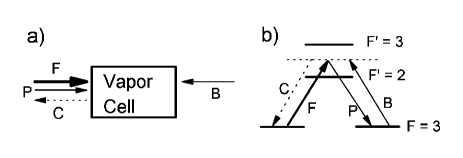
Figure 1: a) Geometry of the DBFWM experiment, beams F and P are copropagating and beam B is counterpropagating with respect to both. Beam C is generated counterpropagating with respect to beam P. b) The effective four level atomic system used in the experiment, with the ground levels corresponding to different Zeeman sublevels of the $F=3$ hyperfine level of Cs$\left(6S_{1/2}\right)$ while the excited states are Zeeman sublevels of the hyperfine $F^{\prime}=2$ and $F^{\prime}=3$ levels of Cs$\left(6P_{3/2}\right)$. F and C have $\sigma_{+}$ circular polarization, while beams B and P have $\sigma_{-}$ polarization.

The experimental setup is depicted in Fig. 2. We use an external cavity diode laser emitting around 852 nm, with linewidth below 1 MHz and output power of about 40 mW. The main beam is sent through an acousto-optical modulator, with its non-deflected beam used as the F beam. The beam deflected in order 1 pass through another acousto-optical modulator (with the same RF frequency as the first one) and the new deflected beam in order -1 is used as beam P. Such setup allows us to scan the frequency of P ($\omega_{P}$) around the frequency of F ($\omega_{F}$). The polarization of F is rotated by $90^{o}$ before it is combined with P using a polarizing beam splitter (PBS). The combined beams pass through a $\lambda/4$ plate producing the desired circular polarizations and are then sent into the cell. The beams diameter at the cell is around 3 mm. The transmitted beams are converted back to linear polarization by a second quarter wave plate and separated by another PBS. After the cube, F is retro-reflected to produce the beam B (with $\omega_{B}=\omega_{F}$). A 50/50 beam splitter is used to reflect the beam C that propagates in opposite direction to P. The laser frequency is monitored using a saturated absorption setup.

The cell used in the four wave mixing experiment is a vacuum sealed 12 cm long glass cell with diameter of 2.5 cm and filled with Cs at room temperature. We have surrounded the cell with a layer of $\mu$-metal in order to reduce spurious effects from residual external magnetic fields.

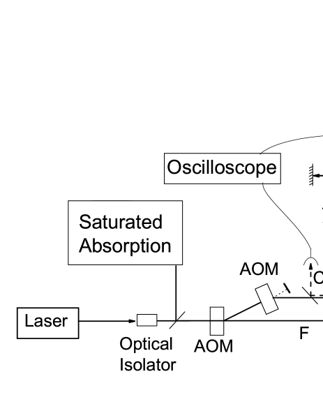
Figure 2: Experimental Setup. PBS means polarizing beam splitter and AOM stands for acousto-optical modulator.

II.2 Experimental results

In Fig. 3 we present typical curves for the detected conjugated-beam intensity ($I_{C}$) as a function of $\omega_{P}$ for fixed values of $\omega_{F}$ and low pump power ($P_{F}=0.1\,$mW). For all our experiments, the pump power will always be given in terms of $P_{F}$, with $P_{B}=0.7\,P_{F}$. Figure 3(a) was obtained for $\omega_{F}$ resonant with the $F=3\rightarrow F^{\prime}=2$ transition ($\omega_{32}$). Figure 3(c) presents a similar signal obtained for $\omega_{F}$ at the crossover resonance between F’=2 and F’=3 ($\omega_{CO}$). For Fig. 3(b), $\omega_{F}$ was chosen between these two values, more precisely at $\omega_{F}=\omega_{32}+2\pi\times 38$ MHz. Note the subnatural linewidth, around 0.8 MHz, of the FWM signal in the three cases. The height of the peak, however, varies with the position of $\omega_{F}$ throughout the Doppler profile, with two maxima at the positions shown in Figs. 3(a) and (c).

The two peaks in Figs. 3(a) and (c) are associated with different atomic level schemes: the peak at transition $\omega_{F}=\omega_{32}$ corresponds mainly to all beams resonant with this transition for atoms with zero velocity along the laser beams, and thus to a three-level $\Lambda$ scheme; the peak at $\omega_{F}=\omega_{CO}$ corresponds mainly to the case where P and F are resonant with the transition $F=3\rightarrow F^{\prime}=2$ ($F=3\rightarrow F^{\prime}=3$) and B is resonant with the transition $F=3\rightarrow F^{\prime}=3$ ($F=3\rightarrow F^{\prime}=2$) for atoms with a velocity component along the beam’s axis of $v_{z}=\frac{\Delta_{F}}{2k}$ ($v_{z}=-\frac{\Delta_{F}}{2k}$), with $\Delta_{F}$ the frequency difference between the two excited levels and k the F-beam wavenumber. Thus, for such velocity class, the system corresponds to a double-$\Lambda$ level scheme. In our experiment, we have then a system that allows us to change the effective experimental atomic level configuration from $\Lambda$ to a double-$\Lambda$ by simply tuning finely the laser frequency.

Figure 3: Intensity of the conjugated beam ($I_{C}$) when $\omega_{P}$ is scanned around a fixed value of $\omega_{F}$ for a) $\omega_{F}=\omega_{32}$, b) $\omega_{F}=\omega_{32}+2\pi\times 38$ MHz, and c) $\omega_{F}=\omega_{CO}$. The powers used for the beams are $P_{F}=100\mu W$, $P_{B}=0.7\,P_{F}$, and $P_{P}=150\mu W$. The same vertical scale was used in all graphs.

When we increase the pump power to $P_{F}=1$ mW, the relative intensities of the conjugated signal for different fixed $\omega_{F}$ exhibit drastic changes (Fig. 4). A strong DBFWM signal occurs when $\omega_{F}$ is between the crossover resonance and $\omega_{32}$, around $2\pi\times 38$ MHz on the blue side of the $F=3\rightarrow F^{\prime}=2$ transition (see Fig. 4(b)). The signal for this frequency is larger than the signal for the $\omega_{F}=\omega_{32}$ resonance (Fig. 4(a)), and the signal for $\omega_{F}=\omega_{CO}$ (Fig. 4(c)) is strongly suppressed. The peaks at Figs. 4(a) and (c) also present a noticeable larger linewidth, indicating stronger power broadening at those conditions.

In order to investigate in detail this dependence of the DBFWM signal for different laser frequencies and power, we measured the peak height (obtained for $\omega_{P}=\omega_{F}$) as a function of $\omega_{F}$ throughout the Doppler profile around the $3\rightarrow 2$ and $3\rightarrow 3$ transitions, and for various pump powers. The results are shown in Fig. 5, together with the saturated absorption signal indicating the value of $\omega_{F}$ at each position. The condition $\omega_{P}=\omega_{F}$ was monitored by measuring a frequency beating in a fast photodiode. From this figure it is possible then to capture the broader picture of the behavior highlighted in Figs. 3 and 4. We clearly observe the two peaks of the DBFWM signal at $\omega_{F}=\omega_{32}$ and $\omega_{F}=\omega_{CO}$ for low pump power (curve (a) for $P_{F}=100\,\mu$W). In addition, we notice that there are also smaller peaks around the two other resonances present in the region scanned by $\omega_{F}$: the transition $F=3\rightarrow F^{\prime}=3$ (at $\omega_{33}$) and the crossover for the transitions $F=3\rightarrow F^{\prime}=2$ and $F=3\rightarrow F^{\prime}=4$. We understand that the $F=3\rightarrow F^{\prime}=3$ peak is largely suppressed due to optical pumping to $F=4$. The smaller height for the $F^{\prime}=2-F^{\prime}=4$ crossover peak should result from a combination of optical pumping and the smaller strenght of the transitions to $F^{\prime}=4$.

Figure 4: Intensity of conjugated beam ($I_{C}$) when the frequency $\omega_{P}$ is scanned around a fixed value of $\omega_{F}$ for a) $\omega_{F}=\omega_{32}$, b) $\omega_{F}=\omega_{32}+2\pi\times 38$ MHz, and c) $\omega_{F}=\omega_{CO}$. The powers used for the beamas are $P_{F}=1$ mW, $P_{B}=0.7\,P_{F}$, and $P_{P}=150\>\mu W$. The same vertical scale was used in all graphs.

Figure 5: Intensity of the conjugated beam while scanning the laser frequency, keeping $\omega_{F}=\omega_{P}=\omega_{B}$. The pump power is equal to: a) $100\mu W$; b) $200\mu W$; c) $400\mu W$ and d) $2000\mu W$. The probe power for curves (a)-(d) is $P_{P}=100\mu W$. The saturated absorption signal used to calibrate the frequency scan is shown in (e).

When the pump power is increased, the power spectrum changes completely (curves (b)-(d) on Figs. 5). The intensity of the conjugate signal ($I_{C}$) at the crossover resonance changes from a peak to a dip, with a similar passage from maximum to minimum occuring around the frequencies $\omega_{32}$ and $\omega_{33}$ for higher pump powers. For high pump powers we obseve now that the largest signals occur in the frequency region between the crossover and the $\omega_{32}$ and $\omega_{33}$ resonances.

III Theoretical model for four wave mixing process

In order to understand the observed dependence of the DBFWM signal with both frequency and power of the pump beams, we developed a theoretical model to calculate the corresponding DBFWM intensity lineshapes. To simplify the notation, we consider levels $|a\rangle$,$|b\rangle$,$|c\rangle$, and $|d\rangle$ as being, respectively, the two degenerated ground states (in our experiment two 6$S_{1/2}$ Zeeman sublevels), and two single Zeeman excited states of levels 6P_3/2 F’=2 and 6P_3/2 F’=3. This corresponds to the simplified four-level scheme depicted in Fig. 1, already used to explain the experimental configuration. According to the beam polarizations, the F beam couples level $|a\rangle$ to levels $|c\rangle$ and $|d\rangle$, while the P and B beams couple level $|b\rangle$ to $|c\rangle$ and $|d\rangle$.

III.0.1 Formalism

We write the system Hamiltonian, in the rotating wave approximation, as:

$$H=H_{0}+V_{F}+V_{B}+V_{P}\,,$$ (1)

with

$$H_{0} = \sum_{j}\hbar\omega_{j}|j\rangle\langle j|\,,$$ (2)

$$V_{F} = \frac{\Omega_{F}\hbar}{2}e^{i\left(\omega^{at}_{F}t-\vec{k}_{F}\cdot\vec{r}\right)}\sum_{j}|a\rangle\langle j|+h.c\,,$$ (3)

$$V_{I} = \frac{\Omega_{I}\hbar}{2}e^{i\left(\omega^{at}_{I}t-\vec{k}_{I}\cdot\vec{r}\right)}\left(|b\rangle\langle c|-|b\rangle\langle d|\right)+h.c\,,$$ (4)

where $j=c,d$; $I=B,P$; $\hbar\omega_{j}$ is the energy of level $|j\rangle$ (levels $|a\rangle$ and $|b\rangle$ are considered at zero energy); $\vec{k}_{I}$ is the wavevector of field $I$; and h.c denotes hermitian conjugated. $\Omega_{F}=\frac{DE_{F}}{\hbar}$ and $\Omega_{I}=\frac{DE_{I}}{\hbar}$ ($I=B,P$) are the modulus of the Rabi frequencies for the various transitions. For simplicity, we have considered the electric dipole moment $D$ with the same modulus for all transitions, but with an opposite sign for the transitions from $|b\rangle$ to $|d\rangle$ (see Ref. Steck for the sign of the different dipole moments). The field frequencies $\omega^{at}_{P}$ and $\omega^{at}_{I}$ are written in the moving atomic frame and are related to the frequencies in the laboratory frame by the Doppler shift: $\omega^{at}_{P}=\omega_{P}-\vec{k}\cdot\vec{v}=\omega^{at}_{F}$ and $\omega^{at}_{B}=\omega_{B}+\vec{k}\cdot\vec{v}$.

We have used the density matrix formalism to calculate the polarization terms responsible for the generation of the conjugated beam. The evolution of the density matrix is given by the Bloch equations:

$$\frac{d}{dt}\rho=-\frac{i}{\hbar}\left[H,\rho\right]+\left(\mbox{r.t.}\right)\,.$$ (5)

To write the relaxation terms (r.t.) we chose to treat the atomic system as closed with both excited states decaying with the same rate $\Gamma$ to the ground states. We also simplify the problem by considering that the excited state has equal probability to decay to each ground state and that the decaying of the coherence $\rho_{ab}$ is given by a relaxation rate $\gamma$, which can be related to the atomic transit time in the cross sections of the beams.

Although in our experiment all the laser beams are cw, the stationary solutions of the Bloch equations cannot be obtained simply imposing $\dot{\rho}_{ij}=0$, since there can be some beating on density matrix elements involving level $|b\rangle$ because beams B and P can have different frequencies (in the atomic frame). To circumvent this problem we have chosen to treat the system of equations perturbatively in $\Omega_{P}$, such that the beating between $\omega^{at}_{P}$ and $\omega^{at}_{B}$ can be neglected. We though consider the following system of equations:

$$\frac{d}{dt}\rho^{(0)} = -\frac{i}{\hbar}\left[H_{0}+V_{F}+V_{B},\rho^{(0)}\right]+\left(\mbox{r.t.}\right)\,,$$ (6)

$$\frac{d}{dt}\rho^{(P)} = -\frac{i}{\hbar}\left[H_{0}+V_{F}+V_{B},\rho^{(P)}\right]-\frac{i}{\hbar}\left[V_{P},\rho^{(0)}\right]$$ (7)

$$+\left(\mbox{r.t.}\right)\,,$$

where $\rho^{(0)}$ and $\rho^{(P)}$ denotes, respectively, density matrix elements in order zero and in order one in $\Omega_{P}$.

From Eqs. (6) and (7) we get two coupled systems of equations containing rotating exponential terms such as $e^{i\left(\omega^{at}_{A}t-\vec{k}_{A}\cdot\vec{r}\right)}$ (where A=F,P,B). To eliminate such terms we introduce the transformationsBloch83 :

$$\rho^{(0)}_{ij} = \sum_{a,b}\sigma^{(0),(a,b)}_{ij}e^{i\left[\left(a\omega^{at}_{F}+b\omega^{at}_{B}\right)t-\left(a\vec{k}_{F}+b\vec{k}_{B}\right)\cdot\vec{r}\right]}\,,$$ (8)

$$\rho^{(P)}_{ij} = \sum_{a,b,c}\sigma^{(P),(a,b,c)}_{ij}\times$$ (9)

$$\;\;\times e^{i\left[\left(a\omega^{at}_{P}+b\omega^{at}_{B}+c\omega^{at}_{P}\right)t-\left(a\vec{k}_{P}+b\vec{k}_{B}+c\vec{k}_{P}\right)\cdot\vec{r}\right]}\,,$$

where $a,b$ are integer numbers and $c=\pm 1$. Introducing such expansion in the optical Bloch equations (Eq. (7)) and looking for stationary solutions, we obtain recurrence relations between the different $\sigma^{(P),(a,b,c)}_{ij}$ and $\sigma^{(0),(a,b)}_{ij}$ coefficients. The conjugated beam in our four wave mixing configuration (see Fig. 1(b)) is generated by the optical coherence terms between the excited levels and the ground level $|a\rangle$ with exponential time and space dependence such that $I_{C}\propto\left|\sigma^{(P),(1,1,-1)}_{ac}+\sigma^{(P),(1,1,-1)}_{ad}\right|^{2}$. We have solved numerically the derived system of recurrence equations and calculated the DBFWM lineshapes by also numerically integrating the corresponding optical coherence over the Maxwellian velocity distribution of the atomic ensemble.

III.0.2 Comparison with experimental results

The calculated DBFWM spectrum for the generated conjugated beam is shown in Fig. 6 for different values of the Rabi frequency of the pump beams.

Figure 6: Calculated spectrum for the conjugated beam intensity as a function of the beam $F$ frequency ($\omega_{F}$) for various Rabi frequencies of the pump beams $\Omega_{F}=\Omega_{B}$: a) $\Omega_{F}=0.01\Gamma$; b) $\Omega_{F}=0.2\Gamma$; c) $\Omega_{F}=0.5\Gamma$; and d) $\Omega_{F}=1.0\Gamma$, where $\Gamma$ is the excited levels decay rate.

For low pump powers the calculated conjugated signal, presented on curve (a) of Fig. 6, exhibits clear peaks for laser frequencies resonant with transitions to the excited levels ($\omega_{c,d}$) and the crossover resonance ($\omega_{CO}$). For higher beam intensities the peaks at $\omega_{F}=\omega_{c,d}$ are deformed and shifted away, while the crossover peak splits in two peaks, with the splitting growing with the beam intensities in curves (b) and (c), and being completely resolved in (d), in a such way that the intensity spectrum shows a dip around $\omega_{F}=\omega_{CO}$.

By comparing to Fig. 5, we observe then a quite good qualitative agreement of the calculated DBFWM lineshapes with the corresponding experimental results. As for the differences between theory and experiment, the most important is the asymmetry of the experimental curves from one side to the other of the crossover resonance. This indicates that the major simplification of our model was not to consider the optical pumping to the $F=4$ ground state, which should lead to the weaking of the signal involving the $F=3\rightarrow F^{\prime}=3$ open transition with respect to the $F=3\rightarrow F^{\prime}=2$ closed transition. We also did not expect to have a quantitative agreement between the experimental and theoretical saturation intensities, since we do not consider the whole Zeeman structure in our model. Taking these effects into consideration, however, we notice that such good qualitative agreement indicates that we have considered in the simplified theory the essential aspects of our experiment, as for the effective four-level system and similar magnitudes of the various dipople moments. Such theory must contain, then, the key elements to explain the experimentally observed behavior.

The main point to be clarified is the reason for having dips at the different atomic resonances, and particularly at $\omega_{CO}$, once the pump power is increased. As for the crossover resonance, one possible reason could be some destructive quantum interference, such that $\sigma^{(P),(1,-1,1)}_{ac}\approx-\sigma^{(P),(1,-1,1)}_{ad}$, due to the fact that for $\omega_{F}=\omega_{CO}$ there are two symmetric quantum pathways for the coherence to be built (due to the two excited levels). However, by examining the individual terms $\sigma^{(P),(1,-1,1)}_{ac}$ and $\sigma^{(P),(1,-1,1)}_{ad}$ issued from our calculations, at $\omega_{F}=\omega_{CO}$ and for different atomic velocity classes, we ruled out such effect. We understand then that the explanation for the dip formation comes from some saturation effect. We envision such saturation coming in the following way. At low intensities, the three observed peaks in Fig. 6 comes from the matching of the two-photon resonance for the transitions induced by $F$ and $P$ with the individual, single-photon resonances of each exciting wave with different atomic levels. At high pump powers, however, the single-photon resonances at $\omega_{c}$ and $\omega_{d}$ are dislocated due to large stark shifts induced by the pump beams. Also, the different stark shifts induced by F and B destroy the two-photon resonance for the $F$ and $P$ fields. In this way, the strongest signal at high pump powers end up occuring for nonresonant frequencies, for which the stark shifts are small and at least the two-photon resonance for $F$ and $P$ is still present.

IV Observation of intensity correlation and anti-correlation

In order to have more insight about the physical mechanisms behind the experimental situation of the last section and to gain knowledge on the possibilities of manipulating the correlation properties of the fields, we have investigated the occurrence of classical intensity correlations between the probe and conjugated beams. We detected then, simultaneously, the transmitted probe intensity and the conjugated beam intensity with a pair of fast photodetectors connected to an also fast, 400 MHz, oscilloscope (see Fig. 2). The beams had similar powers at the detectors, and both the optical paths and the electronic cables carrying the photocurrents were adjusted to have the same lengths. An example of correlated behavior of the conjugated and probe photocurrents is shown in Fig. 7, which displays the signals observed on the oscilloscope as a function of time.

Figure 7: Time fluctuation of a) conjugate and b) probe beam intensities.

In order to characterize such correlations we have calculated the second order correlation function between the two signals defined as Scully05 :

$$G^{(2)}(\tau)=\frac{\left\langle\delta I_{C}(t)\delta I_{P}(t+\tau)\right\rangle}{\sqrt{\left\langle\left[\delta I_{C}(t)\right]^{2}\right\rangle\left\langle\left[\delta I_{P}(t+\tau)\right]^{2}\right\rangle}}$$ (10)

where $I_{P}$ denotes the intensity of the probe beam, and $\left\langle Q(t)\right\rangle=\int_{t}^{t+T}Q(t)dt/T$ denotes the data average over an integration time T. Such function gives quantitative information on the degree of correlation between the two fields, but it has the drawback of mixing all frequency responses and thus giving no information about the spectral behavior of the system. To acquire such information we have also calculated, thus, its corresponding Fourier transform Cruz07 .

In Fig. 8 we show how the crosscorrelation function spectrum is modified for different laser frequencies (we keep $\omega_{F}=\omega_{P}$). The spectra shown are normalized Cruz07 , and in Figs. 8(g) and (h) we provide, respectively, the mean intensity of the conjugated beam and the saturated absorption signal as we scan the laser frequency, indicating the different conditions applied in (a)-(f) with respect to these quantities. We see that for most of the laser frequencies the crosscorrelation function spectrum has positive values, meaning a correlated behavior. For instance, the correlated temporal series shown in Fig. 7 correspond to the spectrum of Fig. 8(b). A different behavior, however, is observed for Fig. 8(c) for which the two beam intensity fluctuations are anti-correlated. Such situation corresponds to the laser frequency at the crossover resonance ($\omega_{CO}$) between $F^{\prime}=2$ and $F^{\prime}=3$.

*[h]

Figure 8: Normalized correlation spectrum for different laser frequencies (with $\omega_{F}=\omega_{P}=\omega_{B}$). The different frequencies analyzed are show by stars in g) and h), where conjugated intensity and saturated absorption signal, respectively, are shown as a function of the scanned laser frequency.

A simple assumption related to propagation effects leading to beams absorption by the atomic vapor can qualitatively explain the different correlated behaviors observed for different laser frequencies. First we should note that the parametric FWM process leads always to intensity correlations in the fluctuation of the probe and conjugate beams since the photons in these modes are generated in pairs. This inherent intensity correlations should compete with the intensity correlation or anti-correlations induced by the differential absorption due to different atomic velocity groups. For the laser frequency at the $F=3\rightarrow F^{\prime}=2$ transition ($\omega_{F}=\omega_{32}$) the main contribution to the conjugated beam intensity comes from atoms with $v_{z}=0$, thus all beams have the same frequency in the atomic frame and couple to the same transition. When the laser frequency fluctuates (phase fluctuation), both beams P and C (detected in our experiment) simultaneously drive away or get closer to the atomic resonance (see Fig. 9(a)). Therefore both beams are equally absorbed by the atomic velocity group with $v_{z}=0$ which tends to increase their intensity correlation. Now if we consider the absorption of these beams by the atomic velocity group $v_{z}>0$, around $v_{z}=0$, for instance, for the situation depicted in ( Fig. 9(a)), the conjugate beam will be closer to resonance than the probe beam and therefore will be more absorbed by this group of atoms, leading to an anti-correlation in the intensity of these beams. However, the absorption of these beams by the symmetric velocity group $v_{z}<0$ will induce an opposite intensity anti-correlation and, as the velocity distribution function is symmetric around $v_{z}=0$, the two contribution will cancel each other. Therefore, we conclude that for the laser frequency at the $F=3\rightarrow F^{\prime}=2$ transition ($\omega_{F}=\omega_{32}$) the intensity fluctuation on the transmission of the probe and conjugate beams should be always correlated due to atomic absorption.

On the other hand, for laser frequencies at the crossover resonance (corresponding to the spectrum of Fig. 8(c)), the main contribution to the conjugate intensity comes from atoms with $v_{z}=v_{CO}=\frac{\Delta_{F}}{2k}$. As before, when the laser frequency fluctuates, for instance, for the case depicted in 9(b) the absorption of the conjugate and probe beams by this atomic velocity group will generate correlation between these two beams. However, differently from the previous case, the absorption of the probe and conjugate beams by the atomic velocity groups symmetrically placed around $v_{CO}$, which induces opposite intensity anti-correlations, will not cancel each other since the atomic velocity distribution around $v_{CO}$ is not symmetric, specifically $f(v_{z}>\frac{\Delta_{F}}{2k})<f(v_{z}<\frac{\Delta_{F}}{2k})$. Thus, we conclude that one can have an overall intensity anti-correlation between the conjugate and the probe beam in this situation.

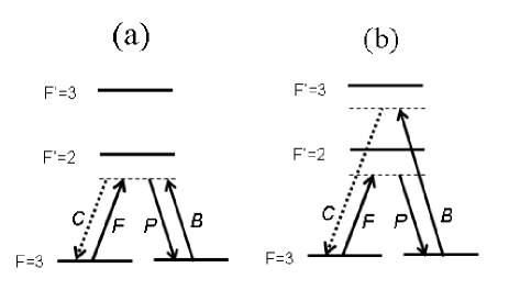
Figure 9: Field frequencies in the atomic moving frame for different laser frequencies and atomic velocity classes. a) $\omega_{F}\approx\omega_{32}$ and $v_{z}=0$; b) $\omega_{F}\approx\omega_{CO}$ and $v_{z}=v_{CO}=\frac{\Delta_{F}}{2k}$.

For laser frequencies between the crossover resonance and a transition to an excited level, such as the situation of spectrum 8(b) where $\omega_{F}=\omega_{32}+2\pi\times(38$ MHz), the analysis is more complicated since the contribution to the generated conjugate intensity comes from different velocity groups. Such correlation measurements, thus, provide another evidence for the different velocity classes contributing to the signal at various conditions. In this way, it highlights once again the possibility of choosing from a three- or a four-level configuration for the generation of the DBFWM signal at a room temperature vapor. It also demonstrates the possibility of manipulating the correlation properties of the generated fields by choosing the position of the pump beams in the Doppler profile.

V Conclusions

We have investigate the four-wave mixing process in a cesium thermal vapor and demonstrated that this simple Doppler broadened system can provide different atomic level configurations for observing this nonlinear phenomenon. We also have developed a theoretical model that reproduces reasonably well the measured FWM spectra. In particular, the possibility of accessing a double -$\Lambda$ level scheme with just a single laser frequency can represent a considerable simplification for the production of quantum correlated photons, whose generation was already demonstrated in similar systems. Towards this direction, we have demonstrated experimentally a strong degree of intensity correlation between the incident probe beam and the generated conjugated beam. Moreover, we have demonstrated that one can switch from correlation to anti-correlation by simply changing the frequency of the incident laser. As noted before, correlation properties between two light beams induced in a coherent EIT media might find application in magnetometry and atomic clocks and we believe our results will certainly broaden this range of applications.

ACKNOWLEDGMENT: We gratefully acknowledge P. J. Ribeiro Neto for his contribution in the early stage of this experiment. This work was supported by the Brazilian Agencies CNPq, CNPq/PRONEX and FACEPE.

References

- (1) S. LeBoiteux, P. Simoneau,D. Bloch, F. A. M. de Oliveira, M. Ducloy, “Saturation behavior of resonant degenerate 4-wave and multiwave mixing in Doppler-Broadenend reginme - Experimental analysis on a low-pressure Ne discharge,” IEEE J. of Quantum Electron. QE-22, 1229 (1986).
- (2) M. D. Lukin,P. R. Hemmer, and M. O. Scully, “Resonant nonlinear optics in phase-coherent media,” Adv. At. Mol. Opt. Phys. 92, 347 (2000).
- (3) J. W. R.Tabosa, S. S. Vianna, and F. A. M. de Oliveira, “Nonlinear spectroscopy and optical phase conjugation in cold cesium atoms”, Phys. Rev. A, 55, 2968 (1997).
- (4) R. L. Abrams, and R. C. Lind, “Degenerate 4-wave mixing in absorbing media,” Opt. Lett. 2, 94 (1978); 3, 205 (1978).
- (5) M. Oria, D. Bloch, M. Ficher, and M. Ducloy, “Efficient phase conjugation of a low-power laser diode in a short Cs vapor cell at 852 nm,” Opt. Lett. 14, 1082 (1989).
- (6) M. Pinard, P. Verkerk, and G. Grynberg, “Backward saturation in four-wave mixing in neon: Case of cross-polarized pumps,” Phys. Rev. A 35, 4679 (1986)
- (7) G. C. Cardoso, and J. W. R. Tabosa, “Electromagnetically induced gratings in a degenerate open two-level system,” Phys. Rev. A 65, 033803 (2002)
- (8) P. R. Hemmer, D. P. Katz, J. Donioghue, M. Cronin-Golomb, M. S. Shahriar, P. Kumar, “Efficient low-intensity optical phase conjugation based on coherent population trapping in sodium,” Opt. Lett. 20, 982 (1995).
- (9) Pavel Kolchin, Shengwang Du, Chinmay Belthangady, G. Y. Yin,and S. E. Harris, “Generation of Narrow-Bandwidth Paired Photons: Use of a Single Driving Laser,” Phys. Rev. Lett. 97, 113602(2006).
- (10) V. Boyer, C. F. McCormick, E. Arimondo, and P. D. Lett, “Generation of Narrow-Bandwidth Paired Photons: Use of a Single Driving Laser,” Phys. Rev. Lett. 99, 143601(2007).
- (11) C. F. McCormick, V. Boyer, E. Arimondo, and P. D. Lett, “Strong relative intensity squeezing by four-wave mixing in rubidium vapor,” Opt. Lett. 32, 178 (2007).
- (12) S.E. Harris, “Electromagnetically induced transparency,” Phys. Today. 50, 36 (1997).
- (13) M. Fleischhauer, A. Imamoglu, and J. P. Marangos, “Electromagnetically induced transparency: Optics in coherent media,” Rev. Mod. Phys. 77, 633 (2005).
- (14) M.D. Lukin, P.R. Hemmer, M. Loffler, and M. O. Scully, “Resonant Enhancement of Parametric Processes via Radiative Interference and Induced Coherence,” Phys. Rev. Lett. 81, 2675(1998).
- (15) M. S. Shahriar, and P.R. Hemmer, “Generation of squeezed states and twin beams via non-degenerate four-wave mixing in a system,” Opt. Communications 158, 273(1998).
- (16) C. Garrido-Alzar, L. S. D. Cruz, J. G. Aguirre-Gómez, M. F. Santos, and P. Nussenzveig, “Super-Poissonian intensity fluctuations and correlations between pump and probe fields in Electromagnetically Induced Transparency,” Europhys. Lett. 61, 485 (2003).
- (17) M. Martinelli, P. Valente, H. Failache, D. Felinto, L. S. Cruz, P. Nussenzveig, and A. Lezama, “Noise spectroscopy of nonlinear magneto-optical resonances in Rb vapor,” Phys. Rev. A 69, 043809(2004).
- (18) Vladimir A. Sautenkov, Yuri V. Rostovtsev, and Marlan O. Scully, “Switching between photon-photon correlations and Raman anticorrelations in a coherently prepared Rb vapor,” Phys. Rev. A 72, 065801(2005).
- (19) D. A. Steck, Cesium D Line Data, http://steck.us/alkalidata.
- (20) D. Bloch, and M. Ducloy, “Theory of saturated line-shapes in phase-conjugate emission by resonant degenerate 4-wave mixing in Doppler-broadened 3-level systems,” J. Opt. Soc. Am. 73, 635 (1983); 73, 1844 (1983).
- (21) L.S. Cruz, D. Felinto, J.G.A. Gomez, M. Martinelli, P. Valente, A. Lezama, P. Nussenzveig, “Laser-noise-induced correlations and anti-correlations in electromagnetically induced transparency,” Euro. Phys. Journal D41, 531(2007).