Parallel-tempering cluster algorithm for computer simulations of critical phenomena

Abstract

In finite-size scaling analyses of Monte Carlo simulations of second-order phase transitions one often needs an extended temperature range around the critical point. By combining the parallel tempering algorithm with cluster updates and an adaptive routine to find the temperature window of interest, we introduce a flexible and powerful method for systematic investigations of critical phenomena. As a result, we gain one to two orders of magnitude in the performance for 2D and 3D Ising models in comparison with the recently proposed Wang-Landau recursion for cluster algorithms based on the multibondic algorithm, which is already a great improvement over the standard multicanonical variant.

I Introduction

While much attention has been paid in the past to simulations of first-order phase transitions and systems with rugged free-energy landscapes in generalized ensembles (umbrella, multicanonical, Wang-Landau, parallel/simulated tempering sampling) rugged , the merits of this non-Boltzmann sampling approach also for simulation studies of critical phenomena have been pointed out only recently. In Ref. bbwj , Berg and one of the authors combined multibondic sampling JaKa95 with the Wang-Landau recursion WaLa01 to cover the complete “desired” critical temperature window in a single simulation for each lattice size, where the “desired” range derives from a careful finite-size scaling (FSS) analysis of all relevant observables.

Recent developments in the field of Graphic Processing Units (GPUs) make it possible to have access to a massively parallel computing solution at a low cost. To use these devices in a most efficient way new parallelized algorithms are needed. Our parallel tempering cluster algorithm is a combination of replica-exchange methods pt with the Swendsen-Wang cluster algorithm sw and is therefore predestinated for use in such devices.

II Parallel-Tempering Cluster Algorithm

For the parallel-tempering procedure of the combined algorithm we use a set of $N_{\rm rep}$ replica, where the number of replica depends on the “desired” range that is needed for the FSS analysis opti . To determine this range we perform at the beginning of our simulations a short run in a reasonable temperature interval. We choose the number of replica $N_{\rm rep}$ such that the acceptance rate $A(1\rightarrow 2)$ between adjacent replica is about 50%, which can be calculated from

$$A(1\rightarrow 2)=\!\!\sum_{E_{1},E_{2}}P_{\beta_{1}}(E_{1})P_{\beta_{2}}(E_{2})P_{\rm PT}(E_{1},\beta_{1}\rightarrow E_{2},\beta_{2}),$$ (1)

where $P_{\beta_{i}}(E_{i})$ is the probability for replica $i$ at inverse temperature $\beta_{i}$ to have energy $E_{i}$ and

$$P_{\rm PT}(E_{1},\beta_{1}\rightarrow E_{2},\beta_{2})=\min[1,\exp(\Delta\beta\Delta E)]$$ (2)

with $\Delta\beta=\beta_{2}-\beta_{1}$, $\Delta E=E_{2}-E_{1}$ is the probability to accept a proposed exchange of different, usually adjacent replica. This choice of $A(1\rightarrow 2)$ ensures that the multi-histogram reweighting multi works properly and the flow in (inverse) temperature space, that is, the rate of round trips between low and high temperatures is optimal opti . This is the main difference to our preliminary note pos , where we used histogram overlaps instead. Using the data of this short run as input for the multi-histogram reweighting routine, we determine the pseudo-critical points $C^{\rm max}=C(\beta^{\rm max}_{C})$ of the specific heat $C(\beta)=\beta^{2}V(\langle e^{2}\rangle-\langle e\rangle^{2})$ and $\chi^{\rm max}$ of the susceptibility $\chi(\beta)=\beta V(\langle m^{2}\rangle-\langle|m|\rangle^{2})$, where $e=E/V$ is the energy density, $m=M/V$ the magnetization density, and $V=L^{d}$ the size of the system. Furthermore, we measured the maxima of the slopes of the magnetic cumulants, $U_{2k}(\beta)=1-\langle m^{2k}\rangle/3\langle|m|^{k}\rangle^{2}$ ($k=1,2$), and of the derivatives of the magnetization, $d\langle|m|\rangle/d\beta$, $d\langle\ln|m|^{k}\rangle/d\beta$ ($k=1,2$), respectively. We also include the first structure factor $S_{k_{1}}$ (see, e.g., Ref. stanly ) in our measurement scheme to allow a direct comparison with the results of Ref. bbwj .

Next we determine $\beta$ values where the observables $S=\{C,\chi,\dots\}$ reach the value $S(\beta^{+/-}_{S})=rS^{\rm max}$ with $r\leq 1$. This leads to a sequence of $\beta^{+/-}_{S}$ values satisfying $\beta^{-}_{S}\leq\beta^{\rm max}_{S}$, and $\beta^{+}_{S}\geq\beta^{\rm max}_{S}$ as illustrated for the two-dimensional (2D) Ising model in Fig. 1. The actual simulation range is then given by the largest interval covered by these $\beta_{S}^{+/-}$ values, i.e., for the example in Fig. 1 the “desired” simulation window would be $[\beta_{S_{k_{1}}}^{-},\beta^{+}_{C}]$.

Figure 1: (Color online) Reweighted observables for the 2D Ising model with $L=8$. The symbols mark the maximum values $S^{\rm max}$ and the value $S(\beta^{+/-}_{S})=rS^{\rm max}$ with $r=2/3$.

In practice we start by estimating for a very small system a reasonable (inverse) temperature interval $[\beta^{-},\beta^{+}]$ and the number of replica $N_{\rm rep}$ by trial and error. For successively larger systems we use the measured temperature interval and $N_{\rm rep}$ of the next smaller system as input parameters. The work flow of our method is then given by the following general recipe:

1. compute the simulation temperatures of the replica equidistant in $\beta$,

2. perform several hundred thermalization sweeps and a short measurement run,

3. check the histogram overlap between adjacent replica: if the overlap is too small ($<10\%$), add a further replica and go back to step 1, else go on,

4. use multi-histogram reweighting to determine $\beta_{S}^{-}$ and $\beta_{S}^{+}$ for all observables $S$, leading to the temperature interval $[\beta_{\rm min}^{-},\beta^{+}_{\rm max}]=[\min_{S}\{\beta_{S}^{-}\},\max_{S}\{\beta_{S}^{+}\}]$,

5. start with $\beta^{-}=\beta_{\rm min}^{-}$ and compute a sequence of temperatures $\beta_{i}$ with fixed acceptance rate $A(1\rightarrow 2)$ until $\beta_{i}=\beta^{+}\geq\beta^{+}_{\rm max}$,

6. perform several thousand thermalization sweeps and a long measurement run.

Table 1: Simulation windows and numbers of replica (see text) for the 2D Ising model simulations with $r=2/3$ on $L^{2}$ lattices.

$L$	$\beta^{-}=\beta_{S_{k_{1}}}^{-}$	$\beta_{\rm max}^{+}=\beta_{C}^{+}$	$\beta^{+}$	$N_{\rm rep}$	$N_{\rm rep}^{*}$
8	0.191 636	0.489 877	0.565 730	7	6
16	0.320 580	0.470 826	0.471 618	7	7
32	0.380 475	0.460 499	0.471 780	9	7
64	0.410 832	0.452 619	0.457 003	10	8
128	0.425 789	0.448 345	0.449 188	11	8
256	0.433 267	0.446 069	0.446 392	13	9
512	0.437 042	0.443 171	0.443 674	14	10
1024	0.438 854	0.442 400	0.442 464	16	10
$\infty$	$\beta_{c}=\ln(1+\sqrt{2})/2=0.440\,686\,7935\dots$

III Results

III.1 2D Ising model

Applying this recipe to the 2D Ising model, our computer program simulated system sizes from $L=8$ up to $L=1024$ fully automatically. This shows how robust our new method is. Table 1 gives an overview of the resulting temperature intervals and the numbers of replica needed when for comparison with Ref. bbwj $r=2/3$ is used. Due to the acceptance rate criterion in step 5 of our iterative procedure, the upper bounds $\beta^{+}$ of the temperature intervals slightly overshoot $\beta_{\rm max}^{+}$ and show relatively large fluctuations. With increasing system sizes this discretization effect becomes less pronounced, see Fig. 2 where we compare the automatically determined interval of our algorithm with the exact temperature interval $[\beta_{C}^{-},\beta^{+}_{C}]$ using the specific-heat formula of Ferdinand and Fisher FF .

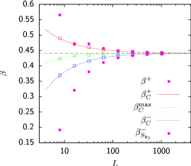
Figure 2: (Color online) The “desired” temperature interval for $r=2/3$ as a function of the system size. The horizontal line indicates the critical inverse temperature $\beta_{c}$, the other lines show exact results derived from Ref. FF . The circles indicate the simulation windows determined fully automatically, cf. Table 1, and the boxes show for completeness the measured values for $\beta_{C}^{+}$, $\beta_{C}^{\rm max}$ and $\beta_{C}^{-}$.

To assess the performance of the method, we measured the integrated autocorrelation times $\tau_{\rm int}(\beta_{i},L)$ and determined the maximum over all replica, $\tau_{\rm int}(L)=\max_{i=1,N_{\rm rep}}\tau_{\rm int}(\beta_{i},L)$, for each lattice size. By fitting the critical slowing down ansatz $\tau_{\rm int}(L)\propto L^{z}$ to the data, we find for $e$, $m^{2}$, and $S_{k_{1}}$ rather small dynamical critical exponents $z=0.19(1)$, $z=0.11(1)$, and $z=0.01(1)$, respectively. As an example, we compare in Fig. 3 our data for $\tau_{{\rm int},E}(L)$ of the energy with the results of Ref. bbwj . Of course, in our case the computational effort depends linearly on the number of replica needed. We therefore also show the effective autocorrelation time $\tau_{\rm eff}=N_{\rm rep}\,\tau_{\rm int}$, which enables a fair comparison in units of lattice sweeps. We see that for $L>100$, our $\tau_{\rm eff}$ is more than one order of magnitude smaller than using the recently proposed multibondic Wang-Landau method bbwj . For $r=2/3$, $N_{\rm rep}$ grows with increasing lattice size $\propto L^{z^{\prime}}$ with $z^{\prime}\approx 0.18$ (cf. Table 1). Consequently, $\tau_{\rm eff}\propto L^{z_{\rm eff}}$ with $z_{\rm eff}=z+z^{\prime}$. For the energy this gives $z_{\rm eff}\approx 0.37$, which is still much smaller than the exponent $z\approx 1.04$ found in Ref. bbwj , so that the gain in efficiency becomes more and more pronounced with increasing lattice size.

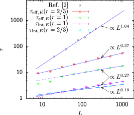
Figure 3: (Color online) Autocorrelation times $\tau_{\rm int}$ and $\tau_{\rm eff}$ for the energy of the 2D Ising model, where $\tau_{\rm eff}=N_{\rm rep}\,\tau_{\rm int}$ with $N_{\rm rep}$ denoting the number of replica, cf. Table 1.

The choice $r=2/3$ of Ref. bbwj is quite conservative as even for $r=1$ the peaks determining the left and right boundary of the “desired” simulation window are usually sufficiently well sampled. This amounts to a somewhat smaller temperature range and repeating the above procedure with $r=1$, we arrive at a smaller $z_{\rm eff}=z=0.27$, see Fig. 3. Here $z_{\rm eff}=z$ because the integer valued $N_{\rm rep}$ turn out be so small (3 for $L=8,16$ and 4 for $32\leq L\leq 1024$) that they practically stay constant over a wide range of system sizes. For large $L$, this leads to a significant gain, and also for the moderate system sizes of Fig. 3, $\tau_{\rm eff}$ is already reduced by a factor of about 3 compared with the case of $r=2/3$ and a factor of about 100 compared with Ref. bbwj .

On the other hand, for $r<2/3$, the “desired” simulation window (and hence also $N_{\rm rep}$) becomes larger, and the effective autocorrelation time $\tau_{\rm eff}$ grows faster with system size. For example for $r=1/2$, we find $z^{\prime}\approx 0.32$. With $z=0.23(1)$ this leads to $z_{\rm eff}=0.55(2)$ for the energy and similar results for $m^{2}$ and $S_{k_{1}}$.

Figure 4: (Color online) FSS of the “desired” simulation window for the 2D Ising model with $r=2/3$.

In order to understand the FSS of $\tau_{\rm eff}$ theoretically, we have to recall that the 2D Ising model is a particular case due to its logarithmic divergence of the specific heat $C$ (with critical exponent $\alpha=0$). First, this leads to a logarithmic correction in the FSS of the reweighting range, $\Delta\beta_{\rm rew}\propto L^{-1/\nu}/\sqrt{\ln L}$. Second, when $C$ is included in the “desired” quantities, it (empirically) determines the upper bound $\beta_{\rm max}^{+}=\beta_{C}^{+}$, which then does not scale generically with $L^{-1/\nu}$ but with $L^{-r/\nu}$ bbwj1 . For the “desired” range $\beta^{+}-\beta^{-}\approx\beta_{C}^{+}-\beta_{S_{k_{1}}}^{-}=aL^{-1/\nu}+bL^{-r/\nu}$, this shows that $L^{-r/\nu}$ is asymptotically the leading term for $r<1$, so that $N_{\rm rep}=(\beta^{+}-\beta^{-})/\Delta\beta_{\rm rew}\rightarrow L^{(1-r)/\nu}\sqrt{\ln L}$ for $L\gtrsim L_{\times}=(a/b)^{\nu/(1-r)}$. However, as Fig. 4 demonstrates for $r=2/3$, this is not observed for practically accessible lattice sizes: Instead of $L^{-2/3}$ (with $\nu=1$) we observe $\beta^{+}-\beta^{-}\propto L^{-\kappa^{\prime}}$ with $\kappa^{\prime}=0.94$. The reason is the very slow crossover from subleading to leading scaling behavior. In fact, whereas both $\beta_{c}-\beta_{S_{k_{1}}}^{-}\propto L^{-1.01}$ and $\beta_{C}^{+}-\beta_{c}\propto L^{-0.69}$ do scale as expected, the asymptotically leading term starts to dominate only at around $L=1000\approx L_{\times}$ with $a/b=10$, which implies $N_{\rm rep}\propto L^{0.06}\sqrt{\ln L}$ for $L\lesssim 1000$. Since in this range to a very good approximation $\sqrt{\ln L}\approx L^{0.11}$ (which can be easily verified directly), this effectively leads to $N_{\rm rep}\propto L^{0.17}$, in good agreement with our direct estimate $z^{\prime}\approx 0.18$. For $r=1/2$, $L^{-1}$ and $L^{-r}=L^{-1/2}$ differ more strongly and we observe the crossover in the FSS of $\beta^{+}-\beta^{-}$ already at about $L=150\approx L_{\times}$ with $a/b=12$, yielding here $\beta^{+}-\beta^{-}\propto L^{-0.80}$ and hence $N_{\rm rep}\propto L^{0.20}\sqrt{\ln L}\approx L^{0.31}$, again as fitted directly. Only for $r=1$, $\beta^{+}-\beta^{-}\propto L^{-1/\nu}$ and $N_{\rm rep}\propto\sqrt{\ln L}$, which as explained above is hardly visible for small (integer) values of $N_{\rm rep}$.

If one omits $C$ as a criterion to specify the “desired” FSS window, both the upper bound $\beta^{+}$ and $\beta^{+}-\beta^{-}$ scale $\propto L^{-1/\nu}$ for any value of $r$, so that $N_{\rm rep}^{*}\propto\sqrt{\ln L}$, see the last column in Table 1 for the case $r=2/3$. If the simulation window is now too narrow to determine the critical exponent $\alpha$ directly, one still can use the hyperscaling relation $\alpha=2-d\nu$ with $d$ the dimensionality. Whereas the “bare” dynamical critical exponents $z$ do not differ much, due to the smaller number of replica needed, $\tau_{\rm eff}=N_{\rm rep}^{*}\,\tau_{\rm int}$ is slightly smaller than in the case including $C$. If one again simply fits a power law to both $\tau_{\rm int}$ and $\tau_{\rm eff}$ (i.e., ignores the logarithmic behavior of $N^{*}_{\rm rep}$), one finds excellent fits with $z=0.20(1)$ and $z_{\rm eff}=0.31(1)=z+0.11$ for the energy ($z=0.11(1)$, $z_{\rm eff}=0.22(1)$ for $m^{2}$ and $z=0.03(1)$, $z_{\rm eff}=0.13(1)$ for $S_{k_{1}}$), confirming that effectively $\sqrt{\ln L}\approx L^{0.11}$ for moderately large $L\lesssim 1000$.

Table 2: Simulation windows and numbers of replica for the 3D Ising model simulations with $r=2/3$ on $L^{3}$ lattices.

$L$	$\beta^{-}=\beta_{S_{k_{1}}}^{-}$	$\beta_{C}^{+}$	$\beta^{+}$	$N_{\rm rep}$
4	0.061 955	0.284 066	0.311 321	7
6	0.142 959	0.259 876	0.272 522	8
8	0.173 712	0.252 866	0.259 229	9
10	0.188 447	0.246 916	0.252 136	10
12	0.197 404	0.241 159	0.243 106	10
16	0.206 422	0.236 610	0.236 773	11
20	0.211 183	0.233 407	0.233 621	12
24	0.213 807	0.232 462	0.233 016	14
28	0.215 553	0.229 853	0.230 301	14
32	0.216 670	0.229 221	0.229 293	15
36	0.217 572	0.228 026	0.228 613	16
40	0.218 172	0.227 703	0.228 025	17
48	0.219 082	0.226 669	0.226 754	18
56	0.219 621	0.225 353	0.225 555	18
64	0.220 031	0.224 758	0.224 775	18
72	0.220 309	0.224 359	0.224 435	19
80	0.220 505	0.224 331	0.224 347	21
$\infty$	$\beta_{c}\simeq 0.221\,654\,59$ (Ref. bloete )

III.2 3D Ising model

In the 3D Ising model where $\alpha\approx 0.11>0$, both the reweighting range and the “desired” temperature window should scale with $L^{-1/\nu}$, so that one would expect that our routine will use the same number of replica for all system sizes. This is indeed the case for the simplest choice $r=1$, where our routine determines for all lattice sizes $N_{\rm rep}=4$. The autocorrelation analysis along the same lines as in 2D gives $z=z_{\rm eff}=0.62(2)$ for the energy ($z=z_{\rm eff}=0.59(2)$ for $m^{2}$ and $z=z_{\rm eff}=0.37(2)$ for $S_{k_{1}}$). This exponent is thus again much smaller than $z\approx 1.05$ obtained in Ref. bbwj , and already for moderate system sizes $L\approx 40-80$ the values of $\tau_{\rm eff}$ are about $20-30$ times smaller, cf. Fig. 5.

If we choose $r=2/3$ as in Ref. bbwj , however, we find also here a weak system-size dependence $N_{\rm rep}\propto L^{0.36}$, cf. Table 2 where also the automatically determined temperature intervals are given. Here we obtain $z=0.44(1)$ and thus $z_{\rm eff}=0.80(1)$ for the energy, cf. Fig. 5 ($z=0.41(1)$, $z_{\rm eff}=0.78(1)$ for $m^{2}$ and $z=0.18(2)$, $z_{\rm eff}=0.55(2)$ for $S_{k_{1}}$). The reason for this unexpected result can be traced back to the fact that the upper boundary $\beta^{+}_{C}$ of the “desired” simulation window, determined by the low-temperature tail of $C$, lies for $r=2/3$ clearly outside the FSS region. In fact, omitting $C$ as a criterion for the FSS window, $N_{\rm rep}=7-9$ stays almost constant. The choice $r<1$ is thus less favorable, but even for $r=2/3$ one gains about one order of magnitude in computing time compared with Ref. bbwj .

Figure 5: (Color online) Same as Fig. 3 for the 3D Ising model, cf. Table 2.

IV Conclusions

To summarize, we have introduced a very flexible and simple approach for a systematic determination and simulation of the critical temperature window of interest for second-order phase transitions, which one needs for an accurate estimation of critical exponents and other quantities characterizing critical phenomena. The efficiency of the method depends of course on the chosen or available update scheme in the particular case, with non-local cluster flips being the favorable choice. Since the setup of our method is completely general and can be combined also with any other update scheme (multigrid, worms, Metropolis, heat-bath, Glauber, $\dots$), it could be employed for all simulations in statistical physics, chemistry and biology, high-energy physics and quantum field theory where one is interested in critical phenomena.

References

- (1) W. Janke (Ed.), Rugged Free Energy Landscapes: Common Computational Approaches to Spin Glasses, Structural Glasses and Biological Macromolecules, Lect. Notes Phys. 736 (Springer, Berlin, 2008).
- (2) B.A. Berg and W. Janke, Phys. Rev. Lett. 98, 040602 (2007).
- (3) W. Janke and S. Kappler, Phys. Rev. Lett. 74, 212 (1995).
- (4) F. Wang and D.P. Landau, Phys. Rev. Lett. 86, 2050 (2001).
- (5) K. Hukushima and K. Nemoto, J. Phys. Soc. Jpn. 65, 1604 (1996).
- (6) R.H. Swendsen and J.-S. Wang, Phys. Rev. Lett. 58, 86 (1987).
- (7) E. Bittner, A. Nußbaumer, and W. Janke, Phys. Rev. Lett. 101, 130603 (2008).
- (8) A.M. Ferrenberg and R.H. Swendsen, Phys. Rev. Lett. 63, 1195 (1989).
- (9) E. Bittner and W. Janke, PoS (LAT2009) 042.
- (10) H.E. Stanley, Introduction to Phase Transitions and Critical Phenomena (Clarendon Press, Oxford, 1971), p. 98.
- (11) A.E. Ferdinand and M.E. Fisher, Phys. Rev. 185, 832 (1969).
- (12) B.A. Berg and W. Janke, Comp. Phys. Comm. 179, 21 (2008).
- (13) H. W. J. Blöte, L. N. Shchur, and A. L. Talapov, Int. J. Mod. Phys. C 10, 1137 (1999).