Model Based Synthesis of Control Software from System Level Formal Specifications

Abstract

Many Embedded Systems are indeed Software Based Control Systems, that is control systems whose controller consists of control software running on a microcontroller device. This motivates investigation on Formal Model Based Design approaches for automatic synthesis of embedded systems control software. We present an algorithm, along with a tool QKS implementing it, that from a formal model (as a Discrete Time Linear Hybrid System) of the controlled system (plant), implementation specifications (that is, number of bits in the Analog-to-Digital, AD, conversion) and System Level Formal Specifications (that is, safety and liveness requirements for the closed loop system) returns correct-by-construction control software that has a Worst Case Execution Time (WCET) linear in the number of AD bits and meets the given specifications. We show feasibility of our approach by presenting experimental results on using it to synthesize control software for a buck DC-DC converter, a widely used mixed-mode analog circuit, and for the inverted pendulum.

1 Introduction

Many Embedded Systems are indeed Software Based Control Systems (SBCS). An SBCS consists of two main subsystems: the controller and the plant. Typically, the plant is a physical system consisting, for example, of mechanical or electrical devices whereas the controller consists of control software running on a microcontroller (see Fig. 2). In an endless loop, the controller reads sensor outputs from the plant and sends commands to plant actuators in order to guarantee that the closed loop system (that is, the system consisting of both plant and controller) meets given safety and liveness specifications (System Level Formal Specifications). Missing such goals can cause failures or damages to the plant, thus making an SBCS a hard real-time system.

Software generation from models and formal specifications forms the core of Model Based Design of embedded software [36]. This approach is particularly interesting for SBCSs since in such a case system level (formal) specifications are much easier to define than the control software behavior itself.

Fig. 2 shows the typical control loop skeleton for an SBCS. Measures from plant sensors go through an Analog-to-Digital (AD) conversion (quantization) before being processed (line 2) and commands from the control software go through a Digital-to-Analog (DA) conversion before being sent to plant actuators (line 8). Basically, the control software design problem for SBCSs consists in designing software implementing functions Control_Law and Controllable_Region computing, respectively, the command to be sent to the plant (line 7) and the set of states on which the Control_Law function works correctly (Fault Detection in line 3). Fig. 2 summarizes the complete closed loop system forming an SBCS.

1.  Every $T$ seconds (sampling time) do

2.     Read AD conversion $\hat{x}$ of plant sensor outputs $x$

3.     If ($\hat{x}$ is not in the Controllable_Region)

4.      Then // Exception (Fault Detected):

5.       Start Fault Isolation and Recovery (FDIR)

6.      Else // Nominal case:

7.       Compute (Control_Law) command $\hat{u}$ from $\hat{x}$

8.       Send DA conversion $u$ of $\hat{u}$ to plant actuators

Figure 1: A typical control loop skeleton.

Figure 2: Software Based Control System.

1.1 The Separation-of-Concerns Approach

For SBCS system level specifications are typically given with respect to the desired behavior of the closed loop system. The control software (that is, Control_Law and Controllable_Region) is designed using a separation-of-concerns approach. That is, Control Engineering techniques (e.g., see [16]) are used to design, from the closed loop system level specifications, functional specifications (control law) for the control software whereas Software Engineering techniques are used to design control software implementing the given functional specifications.

Such a separation-of-concerns approach has several drawbacks.

First, usually control engineering techniques do not yield a formally verified specification for the control law or controllable region when quantization is taken into account. This is particularly the case when the plant has to be modelled as a Hybrid System [10, 5, 31, 9] (that is a system with continuous as well as discrete state changes). As a result, even if the control software meets its functional specifications there is no formal guarantee that system level specifications are met since quantization effects are not formally accounted for.

Second, issues concerning computational resources, such as control software Worst Case Execution Time (WCET), can only be considered very late in the SBCS design activity, namely once the software has been designed. As a result, since the SBCS is a hard real-time system (Fig. 2), the control software may have a WCET greater than the sampling time (line 1 in Fig. 2). This invalidates the schedulability analysis (typically carried out before the control software is completed) and may trigger redesign of the software or even of its functional specifications (in order to simplify its design).

Last, but not least, the classical separation-of-concerns approach does not effectively support design space exploration for the control software. In fact, although in general there will be many functional specifications for the control software that will allow meeting the given system level specifications, the software engineer only gets one to play with. This overconstrains a priori the design space for the control software implementation preventing, for example, effective performance trading (e.g., between number of bits in AD conversion, WCET, RAM usage, CPU power consumption, etc.).

We note that the above considerations also apply to the typical situation where Control Engineering techniques are used to design a control law and then tools like Berkeley’s Ptolemy [24], Esterel’s SCADE [68] or MathWorks Simulink [71] are used to generate the control software. Even when the control law is automatically generated and proved correct (for example, as in [55]) such an approach does not yield any formal guarantee about the software correctness since quantization of the state measurements is not taken into account in the computation of the control law. Thus such an approach cannot answer questions like: 1) Can 8 bit AD be used or instead we need, say, 12 bit AD? 2) Will the control software code run fast enough on a, say, 1 MIPS microcontroller (that is, is the control software WCET less than the sampling time)? 3) What is the controllable region?

The previous considerations motivate research on Software Engineering methods and tools focusing on control software synthesis (rather than on control law synthesis as in Control Engineering). The objective is that from the plant model (as a hybrid system), from formal specifications for the closed loop system behavior (System Level Formal Specifications) and from Implementation Specifications (that is, number of bits used in the quantization process) such methods and tools can generate correct-by-construction control software satisfying the given specifications. This is the focus of the present paper.

For a more in-depth discussion of the literature related to the present paper, we refer the reader to Sect. 9 and Tab. 6.

1.2 Our Main Contributions

We model the controlled system (plant) as a Discrete Time Linear Hybrid System (DTLHS) (see Sect. 3), that is a discrete time hybrid system whose dynamics is defined as a linear predicate (i.e., a boolean combination of linear constraints, see Sect. 2) on its variables. We model system level safety as well as liveness specifications as sets of states defined, in turn, as linear predicates. In our setting, as always in control problems, liveness constraints define the set of states that any evolution of the closed loop system should eventually reach (goal states). Using an approach similar to the one in [34, 35, 1], in [54] we prove that both existence of a controller for a DTLHS and existence of a quantized controller for a DTLHS are undecidable problems. Accordingly, we can only hope for semi- or incomplete algorithms.

We present an algorithm computing a sufficient condition and a necessary condition for existence of a solution to our control software synthesis problem (see Sects. 4 and 5). Given a DTLHS model ${\cal H}$ for the plant, a quantization schema (i.e. how many bits we use for AD conversion) and system level formal specifications, our algorithm (see Sect. 6) will return 1 if they are able to decide if a solution exists or not, and 0 otherwise (unavoidable case since our problem is undecidable). Furthermore, when our sufficient condition is satisfied, we return a pair of C functions (see Sect. 7) Control_Law, Controllable_Region such that: function Control_Law implements a Quantized Feedback Controller (QFC) for ${\cal H}$ meeting the given system level formal specifications and function Controllable_Region computes the set of states on which Control_Law is guaranteed to work correctly (controllable region). While WCET analysis is actually performed after control software generation, our contribution is to supply both functions with a Worst Case Execution Time (WCET) guaranteed to be linear in the number of bits of the state quantization schema (see Sect. 7.1). Furthermore, function Control_Law is robust, that is, it meets the given closed loop requirements notwithstanding (nondeterministic) disturbances such as variations in the plant parameters.

We implemented our algorithm on top of the CUDD package and of the GLPK Mixed Integer Linear Programming (MILP) solver, thus obtaining tool Quantized feedback Kontrol Synthesizer (QKS) (publicly available at [65]). This allows us to present experimental results on using QKS to synthesize robust control software for a widely used mixed-mode analog circuit: the buck DC-DC converter (e.g. see [72]). This is an interesting and challenging example (e.g., see [23], [84]) for automatic synthesis of correct-by-construction control software from system level formal specifications. Moreover, in order to show effectiveness of our approach, we also present experimental results on using QKS for the inverted pendulum [41].

Our experimental results address both computational feasibility and closed loop performances. As for computational feasibility, we show that within about 40 hours of CPU time and within 100MB of RAM we can synthesize control software for a 10-bit quantized buck DC-DC converter. As for closed loop performances, our synthesized control software set-up time (i.e., the time needed to reach the steady state) and ripple (i.e., the wideness of the oscillations around the steady state once this has been reached) compares well with those available from the Power Electronics community [72, 84] and from commercial products [76].

2 Background

We denote with $[n]$ an initial segment $\{1,\ldots,n\}$ of the natural numbers. We denote with $X$ = $[x_{1},\ldots,x_{n}]$ a finite sequence (list) of variables. By abuse of language we may regard sequences as sets and we use $\cup$ to denote list concatenation. Each variable $x$ ranges on a known (bounded or unbounded) interval ${\cal D}_{x}$ either of the reals or of the integers (discrete variables). We denote with ${\cal D}_{X}$ the set $\prod_{x\in X}{\cal D}_{x}$. To clarify that a variable $x$ is continuous (i.e. real valued) we may write $x^{r}$. Similarly, to clarify that a variable $x$ is discrete (i.e. integer valued) we may write $x^{d}$. Boolean variables are discrete variables ranging on the set $\mathbb{B}$ = {0, 1}. We may write $x^{b}$ to denote a boolean variable. Analogously $X^{r}$ ($X^{d}$, $X^{b}$) denotes the sequence of real (integer, boolean) variables in $X$. Unless otherwise stated, we suppose ${\cal D}_{X^{r}}=\mathbb{R}^{|X^{r}|}$ and ${\cal D}_{X^{d}}=\mathbb{Z}^{|X^{d}|}$. Finally, if $x$ is a boolean variable we write $\bar{x}$ for $(1-x)$.

2.1 Predicates

A linear expression $L(X)$ over a list of variables $X$ is a linear combination of variables in $X$ with rational coefficients, $\sum_{x_{i}\in X}{a_{i}x_{i}}$. A linear constraint over $X$ (or simply a constraint) is an expression of the form $L(X)\leq b$, where $L(X)$ is a linear expression over $X$ and $b$ is a rational constant. In the following, we also write $L(X)\geq b$ for $-L(X)\leq-b$.

Predicates are inductively defined as follows. A constraint $C(X)$ over a list of variables $X$ is a predicate over $X$. If $A(X)$ and $B(X)$ are predicates over $X$, then $(A(X)\land B(X))$ and $(A(X)\lor B(X))$ are predicates over X. Parentheses may be omitted, assuming usual associativity and precedence rules of logical operators. A conjunctive predicate is a conjunction of constraints. For conjunctive predicates we will also write: $L(X)=b$ for (($L(X)\leq b$) $\wedge$ ($L(X)\geq b$)) and $a\leq x\leq b$ for $x\geq a\;\land\;x\leq b$, where $x\in X$.

A valuation over a list of variables $X$ is a function $v$ that maps each variable $x\in X$ to a value $v(x)\in{\cal D}_{x}$. Given a valuation $v$, we denote with $X^{\ast}\in{\cal D}_{X}$ the sequence of values $[v(x_{1}),\ldots,v(x_{n})]$. By abuse of language, we call valuation also the sequence of values $X^{\ast}$. A satisfying assignment to a predicate $P$ over $X$ is a valuation $X^{*}$ such that $P(X^{*})$ holds. If a satisfying assignment to a predicate $P$ over $X$ exists, we say that $P$ is feasible. Abusing notation, we may denote with $P$ the set of satisfying assignments to the predicate $P(X)$. Two predicates $P$ and $Q$ over $X$ are equivalent, denoted by $P\equiv Q$, if they have the same set of satisfying assignments.

A variable $x\in X$ is said to be bounded in $P$ if there exist $a$, $b\in{\cal D}_{x}$ such that $P(X)$ implies $a\leq x\leq b$. A predicate $P$ is bounded if all its variables are bounded.

Given a constraint $C(X)$ and a fresh boolean variable (guard) $y\not\in X$, the guarded constraint $y\to C(X)$ (if $y$ then $C(X)$) denotes the predicate $((y=0)\lor C(X))$. Similarly, we use $\bar{y}\to C(X)$ (if not $y$ then $C(X)$) to denote the predicate $((y=1)\lor C(X))$. A guarded predicate is a conjunction of either constraints or guarded constraints. It is possible to show that, if a guarded predicate $P$ is bounded, then $P$ can be transformed into a (bounded) conjunctive predicate, see [53].

2.2 Mixed Integer Linear Programming

A Mixed Integer Linear Programming (MILP) problem with decision variables $X$ is a tuple $(\max,$ $J(X),$ $A(X))$ where: $X$ is a list of variables, $J(X)$ (objective function) is a linear expression on $X$, and $A(X)$ (constraints) is a conjunctive predicate on $X$. A solution to $(\max,J(X),A(X))$ is a valuation $X^{*}$ such that $A(X^{*})$ and $\forall Z\;(A(Z)\;\rightarrow\;(J(Z)\leq J(X^{*})))$. $J(X^{*})$ is the optimal value of the MILP problem. A feasibility problem is a MILP problem of the form $(\max,0,A(X))$. We write also $A(X)$ for $(\max,0,A(X))$. We write $(\min,J(X),A(X))$ for $(\max,-J(X),A(X))$.

In algorithm outlines, MILP solver invocations are denoted by function feasible($A(X)$) that returns True if $A(X)$ is feasible and False otherwise, and function optimalValue($\max$, $J(X)$, $A(X)$) that returns either the optimal value of the MILP problem ($\max$, $J(X)$, $A(X)$) or $+\infty$ if such MILP problem is unbounded or unfeasible.

2.3 Labeled Transition Systems

A Labeled Transition System (LTS) is a tuple ${\cal S}=(S,A,T)$ where $S$ is a (possibly infinite) set of states, $A$ is a (possibly infinite) set of actions, and $T$ : $S$ $\times$ $A$ $\times$ $S$ $\rightarrow$ $\mathbb{B}$ is the transition relation of ${\cal S}$. We say that $T$ (and ${\cal S}$) is deterministic if $T(s,a,s^{\prime})\land T(s,a,s^{\prime\prime})$ implies $s^{\prime}=s^{\prime\prime}$, and nondeterministic otherwise. Let $s\in S$ and $a\in A$. We denote with $\mbox{\rm Adm}({\cal S},s)$ the set of actions admissible in $s$, that is $\mbox{\rm Adm}({\cal S},s)$ = $\{a\in A\;|\;\exists s^{\prime}:T(s,a,s^{\prime})\}$ and with $\mbox{\rm Img}({\cal S},s,a)$ the set of next states from $s$ via $a$, that is $\mbox{\rm Img}({\cal S},s,a)$ = $\{s^{\prime}\in S\;|\;T(s,a,s^{\prime})\}$. We call transition a triple $(s,a,s^{\prime})\in S$ $\times$ $A$ $\times$ $S$, and self loop a transition $(s,a,s)$. A transition $(s,a,s^{\prime})$ [self loop $(s,a,s)$] is a transition [self loop] of ${\cal S}$ iff $T(s,a,s^{\prime})$ [$T(s,a,s)$]. A run or path for an LTS ${\cal S}$ is a sequence $\pi$ = $s_{0},a_{0},s_{1},a_{1},s_{2},a_{2},\ldots$ of states $s_{t}$ and actions $a_{t}$ such that $\forall t\geq 0$ $T(s_{t},a_{t},s_{t+1})$. The length $|\pi|$ of a finite run $\pi$ is the number of actions in $\pi$. We denote with $\pi^{(S)}(t)$ the $(t+1)$-th state element of $\pi$, and with $\pi^{(A)}(t)$ the $(t+1)$-th action element of $\pi$. That is $\pi^{(S)}(t)$ = $s_{t}$, and $\pi^{(A)}(t)$ = $a_{t}$.

Given two LTSs ${\cal S}_{1}$ $=$ $(S$, $A$, $T_{1})$ and ${\cal S}_{2}$ $=$ $(S$, $A$, $T_{2})$, we say that ${\cal S}_{1}$ refines ${\cal S}_{2}$ (denoted by ${\cal S}_{1}\sqsubseteq{\cal S}_{2}$) iff $T_{1}(s,a,s^{\prime})$ implies $T_{2}(s,a,s^{\prime})$ for each state $s,s^{\prime}\in S$ and action $a\in A$. The refinement relation is a partial order on LTSs.

3 Discrete Time Linear Hybrid Systems

In this section we introduce our class of Discrete Time Linear Hybrid System (DTLHS), together with the DTLHS representing the buck DC-DC converter on which our experiments will focus.

Definition 3.1 (DTLHS).

A Discrete Time Linear Hybrid System is a tuple ${\cal H}=(X,$ $U,$ $Y,$ $N)$ where:

• $X$ = $X^{r}\cup X^{d}$ is a finite sequence of real ($X^{r}$) and discrete ($X^{d}$) present state variables. We denote with $X^{\prime}$ the sequence of next state variables obtained by decorating with ^′ all variables in $X$.

• $U$ = $U^{r}\cup U^{d}$ is a finite sequence of input variables.

• $Y$ = $Y^{r}\cup Y^{d}$ is a finite sequence of auxiliary variables. Auxiliary variables are typically used to model modes (e.g., from switching elements such as diodes) or “local” variables.

• $N(X,U,Y,X^{\prime})$ is a conjunctive predicate over $X\cup U\cup Y\cup X^{\prime}$ defining the transition relation (next state) of the system. $N$ is deterministic if $N(x,u,y_{1},x^{\prime})\land N(x,u,y_{2},x^{\prime\prime})$ implies $x^{\prime}=x^{\prime\prime}$, and nondeterministic otherwise.

A DTLHS is bounded if predicate $N$ is bounded. A DTLHS is deterministic if $N$ is deterministic.

Since any bounded guarded predicate can be transformed into a conjunctive predicate (see Sect. 2.1), for the sake of readability we will use bounded guarded predicates to describe the transition relation of bounded DTLHSs. To this aim, we will also clarify which variables are boolean, and thus may be used as guards in guarded constraints.

Example 3.2.

Let $x$ be a continuous variable, $u$ be a boolean variable, and $N(x,u,x^{\prime})\equiv[\overline{u}\rightarrow x^{\prime}=\alpha x]\land[u\rightarrow x^{\prime}=\beta x]\land-4\leq x\leq 4$ be a guarded predicate with $\alpha=\frac{1}{2}$ and $\beta=\frac{3}{2}$. Then ${\cal H}=(\{x\},\{u\},\varnothing,N)$ is a bounded DTLHS. Note that ${\cal H}$ is deterministic. Adding nondeterminism to ${\cal H}$ allows us to address the problem of (bounded) variations in the DTLHS parameters. For example, variations in the parameter $\alpha$ can be modelled with a tolerance $\rho\in[0,1]$ for $\alpha$. This replaces $N$ with: $N^{(\rho)}\equiv[\overline{u}\rightarrow x^{\prime}\leq(1+\rho)\alpha x]$ $\land$ $[\overline{u}\rightarrow x^{\prime}\geq(1-\rho)\alpha x]$ $\land$ $[u\rightarrow x^{\prime}=\beta x]$. We have that ${\cal H}^{(\rho)}=(\{x\},\{u\},\varnothing,N^{(\rho)})$, for $\rho\in(0,1]$, is a nondeterministic DTLHS. Note that, as expected, ${\cal H}^{(0)}={\cal H}$.

In the following definition, we give the semantics of DTLHSs in terms of LTSs.

Definition 3.3 (DTLHS dynamics).

Let ${\cal H}$ = ($X$, $U$, $Y$, $N$) be a DTLHS. The dynamics of ${\cal H}$ is defined by the Labeled Transition System $\mbox{\rm LTS}({\cal H})$ = (${\cal D}_{X}$, ${\cal D}_{U}$, $\tilde{N}$) where: $\tilde{N}:{\cal D}_{X}\;\times\;{\cal D}_{U}\;\times\;{\cal D}_{X}\rightarrow\mathbb{B}$ is a function s.t. $\tilde{N}(x,u,x^{\prime})\equiv\exists y\in{\cal D}_{Y}:N(x,u,y,x^{\prime})$. A state $x$ for ${\cal H}$ is a state $x$ for $\mbox{\rm LTS}({\cal H})$ and a run (or path) for ${\cal H}$ is a run for $\mbox{\rm LTS}({\cal H})$ (Sect. 2.3).

Example 3.4.

Let ${\cal H}$ be the DTLHS of Ex. 3.2. Then a sequence $\pi$ is a run for ${\cal H}$ iff state $\pi^{(S)}(i+1)$ is obtained by multiplying $\pi^{(S)}(i)$ by $\frac{3}{2}$ when $\pi^{(A)}(i)=1$, and by $\frac{1}{2}$ when $\pi^{(A)}(i)=0$.

3.1 Buck DC-DC Converter as a DTLHS

The buck DC-DC converter (Fig. 3) is a mixed-mode analog circuit converting the DC input voltage ($V_{i}$ in Fig. 3) to a desired DC output voltage ($v_{O}$ in Fig. 3). As an example, buck DC-DC converters are used off-chip to scale down the typical laptop battery voltage (12-24) to the just few volts needed by the laptop processor (e.g. [72]) as well as on-chip to support Dynamic Voltage and Frequency Scaling (DVFS) in multicore processors (e.g. [40, 70]). Because of its widespread use, control schemas for buck DC-DC converters have been widely studied (e.g. see [40, 70, 72, 84]). The typical software based approach (e.g. see [72]) is to control the switch $u$ in Fig. 3 (typically implemented with a MOSFET) with a microcontroller.

Figure 3: Buck DC-DC converter.

Designing the software to run on the microcontroller to properly actuate the switch is the control software design problem for the buck DC-DC converter in our context.

The circuit in Fig. 3 can be modeled as a DTLHS ${\cal H}$ = ($X$, $U$, $Y$, $N$) in the following way [51].As for the sets of variables, we have $X$ $=$ $X^{r}$ $=$ $[i_{L}$, $v_{O}]$, $U$ $=$ $U^{b}$ $=$ $[u]$, $Y$ $=$ $Y^{r}\cup Y^{b}$ with $Y^{r}$ $=$ $[i_{u}$, $v_{u}$, $i_{D}$, $v_{D}]$ and $Y^{b}$ $=$ $[q]$. As for $N$, it is given by the conjunction of the following (guarded) constraints:

$${i_{L}}^{\prime} = (1+Ta_{1,1})i_{L}+Ta_{1,2}v_{O}+Ta_{1,3}v_{D}$$ (1)

$${v_{O}}^{\prime} = Ta_{2,1}i_{L}+(1+Ta_{2,2})v_{O}+Ta_{2,3}v_{D}.$$ (2)

$\displaystyle q$ $\displaystyle\rightarrow$ $\displaystyle v_{D}=0$ (3) $\displaystyle q$ $\displaystyle\rightarrow$ $\displaystyle i_{D}\geq 0$ (4) $\displaystyle u$ $\displaystyle\rightarrow$ $\displaystyle v_{u}=0$ (5)

$\displaystyle i_{D}$ $\displaystyle=$ $\displaystyle i_{L}-i_{u}$ (6) $\displaystyle\bar{q}$ $\displaystyle\rightarrow$ $\displaystyle v_{D}\leq 0$ (7) $\displaystyle\bar{q}$ $\displaystyle\rightarrow$ $\displaystyle v_{D}=R_{off}i_{D}$ (8)

$\displaystyle\bar{u}$ $\displaystyle\rightarrow$ $\displaystyle v_{u}=R_{off}i_{u}$ (9) $\displaystyle v_{D}$ $\displaystyle=$ $\displaystyle v_{u}-V_{i}$ (10)

where the coefficients $a_{i,j}$ depend on the circuit parameters $R$, $r_{L}$, $r_{C}$, $L$ and $C$ in the following way: $a_{1,1}=-\frac{r_{L}}{L}$, $a_{1,2}=-\frac{1}{L}$, $a_{1,3}=-\frac{1}{L}$, $a_{2,1}=\frac{R}{r_{c}+R}[-\frac{r_{c}r_{L}}{L}+\frac{1}{C}]$, $a_{2,2}=\frac{-1}{r_{c}+R}[\frac{r_{c}R}{L}+\frac{1}{C}]$, $a_{2,3}=-\frac{1}{L}\frac{r_{c}R}{r_{c}+R}$.

4 Quantized Feedback Control

In this section, we formally define the Quantized Feedback Control Problem for DTLHSs (Sect. 4.3). To this end, first we give the definition of Feedback Control Problem for LTSs (Sect. 4.1), and then for DTLHSs (Sect. 4.2). Finally, we show that our definitions are well founded (Sect. 4.4).

4.1 Feedback Control Problem for LTSs

We begin by extending to possibly infinite LTSs the definitions in [80, 20] for finite LTSs. In what follows, let ${\cal S}=(S,A,T)$ be an LTS, and $I,G\subseteq S$ be, respectively, the initial and goal regions.

Definition 4.1 (LTS control problem).

A controller for an LTS ${\cal S}$ is a function $K:S\times A\to\mathbb{B}$ such that $\forall s\in S$, $\forall a\in A$, if $K(s,a)$ then $a\in{\rm Adm}({\cal S},s)$. We denote with $\mbox{\rm Dom}(K)$ the set of states for which a control action is defined. Formally, $\mbox{\rm Dom}(K)$ $=$ $\{s\in S\;|\;$$\exists a:K(s,a)\}.$ ${\cal S}^{(K)}$ denotes the closed loop system, that is the LTS $(S,A,T^{(K)})$, where $T^{(K)}(s,a,s^{\prime})=T(s,a,s^{\prime})\wedge K(s,a)$. A control law for a controller $K$ is a (partial) function $k:S\rightarrow A$ s.t. for all $s\in{\rm Dom}(K)$ we have that $K(s,k(s))$ holds. By abuse of language we say that a controller is a control law if for all $s\in S$, $a,b\in A$ it holds that $(K(x,a)\wedge K(x,b))\rightarrow(a=b)$. An LTS control problem is a triple $({\cal S},$ $I,$ $G)$.

Example 4.2.

Let $S=\{-1,0,1\}$ and $A=\{0,1\}$. Let ${\cal S}_{0}$ be the LTS $(S,A,T_{0})$, where the transition relation $T_{0}$ consists of the continuous arrows in Fig. 4. A function $K$ is a controller for ${\cal S}_{0}$ iff $(s\neq 0)\to(K(s,1)=0)$. As an example, we have that $K$ defined as $K(s,a)=((s\neq 0)\to(a\neq 1))$ is a controller but not a control law, and that $k(s)=0$ is a control law for $K$ (note that $K(s,a)=(a=0)$ is a control law).

Def. 4.1 also introduces the formal definition of control law, as our model of control software, i.e. of how function Control_Law in Fig. 2 must behave. Namely, while a controller may enable many actions in a given state, a control law (i.e. the final software implementation) must provide only one action. Note that the notion of controller is important because it contains all possible control laws.

In the following we give formal definitions of strong and weak solutions to a control problem for an LTS.

We call a path $\pi$ fullpath if either it is infinite or its last state $\pi^{(S)}(|\pi|)$ has no successors (i.e. $\mbox{\rm Adm}({\cal S},\pi^{(S)}(|\pi|))=\varnothing$). We denote with ${\rm Path}({\cal S},s,a)$ the set of fullpaths of ${\cal S}$ starting in state $s$ with action $a$, i.e. the set of fullpaths $\pi$ such that $\pi^{(S)}(0)=s$ and $\pi^{(A)}(0)=a$.

Given a path $\pi$ in ${\cal S}$, we define the measure $J({\cal S},G,\pi)$ on paths as the distance of $\pi^{(S)}(0)$ to the goal on $\pi$. That is, if there exists $n>0$ s.t. $\pi^{(S)}(n)\in G$, then $J({\cal S},G,\pi)$ $=$ $\min\{n$ $|$ $n>0\land\pi^{(S)}(n)\in G\}$. Otherwise, $J({\cal S},G,\pi)=+\infty$. We require $n>0$ since our systems are nonterminating and each controllable state (including a goal state) must have a path of positive length to a goal state. Taking $\sup\varnothing=+\infty$ and $\inf\varnothing=-\infty$, the worst case distance (pessimistic view) of a state $s$ from the goal region $G$ is $J_{\rm strong}({\cal S},G,s)=\sup\{J^{(S)}({\cal S},G,s,a)~{}|~{}a\in{\rm Adm}({\cal S},s)\}$, where: $J^{(S)}({\cal S},G,s,a)=\sup\{J({\cal S},G,\pi)~{}|~{}\pi\in{\rm Path}({\cal S},s,a)\}$. The best case distance (optimistic view) of a state $s$ from the goal region $G$ is $J_{\rm weak}({\cal S},G,s)$ $=$ $\sup\{J^{(W)}({\cal S},G,s,a)$ $|$ $a\in{\rm Adm}({\cal S},s)\}$, where: $J^{(W)}({\cal S},G,s,a)$ $=$ $\inf\{J({\cal S},G,\pi)$ $|$ $\pi\in{\rm Path}({\cal S},s,a)\}$.

Definition 4.3 (Solution to LTS control problem).

Let ${\cal P}$ = $({\cal S}$, $I$, $G)$ be an LTS control problem and $K$ be a controller for ${\cal S}$ such that $I$ $\subseteq$ $\mbox{\rm Dom}(K)$. $K$ is a strong [weak] solution to ${\cal P}$ if for all $s\in\mbox{\rm Dom}(K)$, $J_{\rm strong}({\cal S}^{(K)},G,s)$ [$J_{\rm weak}({\cal S}^{(K)},G,s)$] is finite. An optimal strong [weak] solution to ${\cal P}$ is a strong [weak] solution $K^{*}$ to ${\cal P}$ such that for all strong [weak] solutions $K$ to ${\cal P}$, for all $s\in S$ we have that $J_{\rm strong}({\cal S}^{(K^{*})},G,s)\leq J_{\rm strong}({\cal S}^{(K)},G,s)$ [$J_{\rm weak}({\cal S}^{(K^{*})},G,s)\leq J_{\rm weak}({\cal S}^{(K)},G,s)$].

Intuitively, a strong solution $K$ takes a pessimistic view by requiring that for each initial state, all runs in the closed loop system ${\cal S}^{(K)}$ reach the goal, no matter nondeterministic outcomes. A weak solution $K$ takes an optimistic view about nondeterminism: it just asks that for each action $a$ enabled in a given state $s$, there exists at least a path in ${\rm Path}({\cal S}^{(K)},s,a)$ leading to the goal. Unless otherwise stated, we say solution for strong solution.

Finally, we define the most general optimal strong [weak] solution to ${\cal P}$ (strong [weak] mgo in the following) as the unique strong [weak] optimal solution to ${\cal P}$ enabling as many actions as possible (i.e., the most liberal one). In Sect. 4.4 we show that the definition of mgo is well posed.

Example 4.4.

Let ${\cal S}_{0},{\cal S}_{1}$ be the LTSs in Fig. 4 (see also Ex. 4.2). Let ${\cal P}_{0}=({\cal S}_{0},I,G)$ and ${\cal P}_{1}=({\cal S}_{1},I,G)$ be two control problems, where $I$ $=$ $\{-1,0,1\}$ and $G$ $=$ $\{0\}$. The controller $K(s,a)\equiv[s\neq 0\to a=0]$ is a strong solution to the control problem ${\cal P}_{0}$. Observe that $K$ is not optimal. Indeed, the controller $\tilde{K}(s,a)\equiv a=0$ is such that $J_{\rm strong}({\cal S}^{(\tilde{K})}_{0},G,0)=1<2=J_{\rm strong}({\cal S}^{(K)}_{0},G,0)$. The control problem ${\cal P}_{1}$ has no strong solution. As a matter of fact, to drive the system to the goal region $\{0\}$, any solution $K$ must enable action $0$ in states $-1$ and $1$: in such a case, however, we have that $J_{\rm strong}({\cal S}^{(K)}_{1},\hat{G},1)$ $=$ $J_{\rm strong}({\cal S}^{(K)}_{1},\hat{G},-1)$ $=$ $\infty$ because of the self loops $(1,0,1)$ and $(-1,0,-1)$ of $T_{1}$. Finally, note that $K$ is the weak mgo for ${\cal P}_{1}$ and $\tilde{K}$ is the strong mgo for ${\cal P}_{0}$.

Figure 4: LTSs ${\cal S}_{0}$ (continuous arrows) and ${\cal S}_{1}$ (all arrows). Double circle represents the goal state.

Remark 4.5.

Note that if $K$ is a strong solution to $({\cal S}$, $I$, $G)$ and $G\subseteq I$ (as is usually the case in control problems) then ${\cal S}^{(K)}$ is stable from $I$ to $G$, that is each run in ${\cal S}^{(K)}$ starting from a state in $I$ leads to a state in $G$. In fact, from Def. 4.3 we have that each state $s\in I$ reaches a state $s^{\prime}\in G$ in a finite number of steps. Moreover, since $G\subseteq I$, we have that any state $s\in G$ reaches a state $s^{\prime}\in G$ in a finite number of steps. Thus, any path starting in $I$ in the closed loop system ${\cal S}^{(K)}$ touches $G$ an infinite number of times (liveness).

4.2 Feedback Control Problem for DTLHSs

A control problem for a DTLHS ${\cal H}$ is the LTS control problem induced by the dynamics of ${\cal H}$. For DTLHSs, we only consider control problems where $I$ and $G$ can be represented as predicates over present state variables of ${\cal H}$.

Definition 4.6 (DTLHS control problem).

Given a DTLHS ${\cal H}=(X,U,Y,N)$ and predicates $I$ and $G$ over $X$, the DTLHS (feedback) control problem $({\cal H},I,G)$ is the LTS control problem $(LTS({\cal H}),I,G)$. Thus, a controller $K:{\cal D}_{X}\times{\cal D}_{U}\to\mathbb{B}$ is a strong [weak] solution to $({\cal H},I,G)$ iff it is a strong [weak] solution to $(LTS({\cal H}),I,G)$.

For DTLHS control problems, usually robust controllers are desired. That is, controllers that, notwithstanding nondeterminism in the plant (e.g. due to parameter variations, see Ex. 3.2), drive the plant state to the goal region. For this reason we focus on strong solutions.

Observe that the feedback controller for a DTLHS will only measure present state variables (e.g., output voltage and inductor current in Sect. 3.1) and will not measure auxiliary variables (e.g. diode state in Sect. 3.1).

Example 4.7.

The typical goal of a controller for the buck DC-DC converter in Sect. 3.1 is keeping the output voltage $v_{O}$ close enough to a given reference value $V_{\rm ref}$. This leads to the DTLHS control problem ${\cal P}$ = $({\cal H}$, $I$, $G)$ where ${\cal H}$ is defined in Sect. 3.1, $I\equiv$ $(|i_{L}|\leq 2)$ $\wedge$ $(0\leq v_{O}\leq 6.5)$, $G\equiv$ $(|v_{O}-V_{\rm ref}|\leq\theta)$ $\wedge$ $(|i_{L}|\leq 2)$, and $\theta=0.01$ is the desired buck precision.

4.3 Quantized Feedback Control Problem

Software running on a microcontroller (control software in the following) cannot handle real values. For this reason real valued state feedback from plant sensors undergoes an Analog-to-Digital (AD) conversion before being sent to the control software. This process is called quantization (e.g. see [26] and citations thereof). A Digital-to-Analog (DA) conversion is needed to transform the control software digital output into real values to be sent to plant actuators. In the following, we formally define quantized solutions to a DTLHS feedback control problem.

Definition 4.8 (Quantization function).

A quantization function $\gamma$ for a real interval $I=[a,b]$ is a non-decreasing function $\gamma:[a,b]\to\hat{I}$, where $\hat{I}$ is a bounded integer interval $[\gamma(a),\gamma(b)]\subseteq\mathbb{Z}$. The quantization step of $\gamma$, denoted by $\|\gamma\|$, is defined as $\sup\{\;|w-z|\;|\;w,z\in I\land\gamma(w)=\gamma(z)\}$.

For ease of notation, we extend quantizations to integer intervals, by stipulating that in such a case the quantization function is the identity function (i.e. $\gamma(x)=x$). Note that, with this convention, the quantization step on an integer interval is always $0$.

Definition 4.9 (Quantization for DTLHSs).

Let ${\cal H}=(X,U,Y,N)$ be a DTLHS, and let $W=X\cup U$. A quantization ${\cal Q}$ for $\cal H$ is a pair $(A,\Gamma)$, where:

• $A$ is a predicate of form $\wedge_{w\in W}(a_{w}\leq w\leq b_{w})$ with $a_{w},b_{w}\in{\cal D}_{w}$. For each $w\in W$, we define $A_{w}=\{v\in{\cal D}_{w}\;|\;a_{w}\leq v\leq b_{w}\}$ as the admissible region for variable $w$. Moreover, we define $A_{V}=\prod_{v\in V}A_{v}$, with $V\subseteq W$, as the admissible region for variables in $V$.

• $\Gamma$ is a set of maps $\Gamma=\{\gamma_{w}$ $|$ $w\in W$ and $\gamma_{w}$ is a quantization function for $A_{w}\}$.

Let $V=[w_{1},\ldots,w_{k}]$ and $v=[v_{1},\ldots,v_{k}]\in A_{V}$, where $V\subseteq W$. We write $\Gamma(v)$ (or $\hat{v}$) for the tuple $[\gamma_{w_{1}}(v_{1}),$ $\ldots,$ $\gamma_{w_{k}}(v_{k})]$ and $\Gamma^{-1}(\hat{v})$ for the set $\{v\in A_{V}$ $|$ $\Gamma(v)=\hat{v}\}$. Finally, the quantization step $\|\Gamma\|$ for $\Gamma$ is defined as $\sup\{\;\|\gamma\|\;|\;\gamma\in\Gamma\}$.

For ease of notation, in the following we will also consider quantizations for primed variables $x^{\prime}\in X^{\prime}$, by stipulating that $\gamma_{x^{\prime}}\equiv\gamma_{x}$.

Example 4.10.

Let ${\cal H}$ be the DTLHS described in Ex. 3.2. Let us consider the quantization ${\cal Q}=(A,\Gamma)$, where $A\equiv$ $-2.5\leq x\leq 2.5\land 0\leq u\leq 1$. $A$ defines the admissible region $A_{x}=A_{X}=[-2.5,2.5]$. Let $\Gamma=\{\gamma_{x},\gamma_{u}\}$, with $\gamma_{x}(x)=round(x/2)$ (where $round(x)=\lfloor x\rfloor+\lfloor 2(x-\lfloor x\rfloor)\rfloor$ is the usual rounding function) and $\gamma_{u}(u)=u$. Note that $\gamma_{x}(x)=-1$ for all $x\in[-2.5,-1]$, $\gamma_{x}(x)=0$ for all $x\in(-1,1)$ and $\gamma_{x}(x)=1$ for all $x\in[1,2.5]$. Thus, we have that $\Gamma(A_{x})=\{-1,0,1\}$, $\Gamma(A_{u})=\{0,1\}$ and $\|\Gamma\|$ = 1.

Quantization, i.e. representing reals with integers, unavoidably introduces errors in reading real-valued plant sensors in the control software. We address this problem in the following way. First, we introduce the definition of $\varepsilon$-solution. Essentially, we require that the controller drives the plant “near enough” (up to a given error $\varepsilon$) to the goal region $G$.

Definition 4.11 ($\varepsilon$-relaxation of a set).

Let $\varepsilon\geq 0$ be a real number and $W\subseteq\mathbb{R}^{n}\times\mathbb{Z}^{m}$. The $\varepsilon$-relaxation of $W$ is the set (ball of radius $\varepsilon$) ${\cal B}_{\varepsilon}(W)$ = $\{(z_{1},\ldots z_{n}$, $q_{1},\ldots q_{m})$ $|$ $\exists(x_{1}$, $\ldots$, $x_{n}$, $q_{1}$, $\ldots,q_{m}):(x_{1}$, $\ldots$, $x_{n}$, $q_{1}$, $\ldots$, $q_{m})\in W$ and $\forall i\in\{1,\ldots n\}\;|z_{i}-x_{i}|\leq\varepsilon\}$.

Definition 4.12 ($\varepsilon$-solution to DTLHS control problem).

Let ${\cal P}=({\cal H},I,G)$ be a DTLHS control problem and let $\varepsilon>0$ be a real number. A strong [weak] $\varepsilon$-solution to ${\cal P}$ is a strong [weak] solution to the LTS control problem $(LTS({\cal H}),I,{\cal B}_{\varepsilon}(G))$.

Example 4.13.

Let ${\cal H}$ be the DTLHS described in Ex. 3.2. We consider the control problem defined by the initial region $I=[-2.5,2.5]$ and the goal region $G=\{0\}$ (represented by the predicate $x=0$). The DTLHS control problem ${\cal P}$ $=$ $({\cal H},I,G)$ has no solution (because of the Zeno phenomenon), but for all $\varepsilon>0$ it has the $\varepsilon$-solution $K$ such that $\forall x\in I.\;K(x,0)$.

Second, we introduce the definition of quantized solution to a DTLHS control problem for a given quantization ${\cal Q}=(A,\Gamma)$. Essentially, a quantized solution models the fact that in an SBCS control decisions are taken by the control software by just looking at quantized state values. Despite this, a quantized solution guarantees that each DTLHS initial state reaches a DTLHS goal state (up to an error at most $\|\Gamma\|$).

Definition 4.14 (Quantized Feedback Control solution to DTLHS control problem).

Let ${\cal H}=(X,U,Y,N)$ be a DTLHS, ${\cal Q}=(A,\Gamma)$ be a quantization for ${\cal H}$ and ${\cal P}=({\cal H},I,G)$ be a DTLHS control problem. A ${\cal Q}$ Quantized Feedback Control (QFC) strong [weak] solution to ${\cal P}$ is a strong [weak] $\|\Gamma\|$-solution $K:{\cal D}_{X}\times{\cal D}_{U}\to\mathbb{B}$ to ${\cal P}$ such that $K(x,u)=0$ if $(x,u)\notin A_{X}\times A_{U}$, and otherwise $K(x,u)=\hat{K}(\Gamma(x),\Gamma(u))$ where $\hat{K}:\Gamma(A_{X})\times\Gamma(A_{U})$ $\rightarrow$ $\mathbb{B}$.

Note that a ${\cal Q}$ QFC solution to a DTLHS control problem does not work outside the admissible region defined by ${\cal Q}$. This models the fact that controllers for real-world systems must maintain the plant inside given bounds (such requirements are part of the safety specifications). In the following, we will define ${\cal Q}$ QFC solutions by only specifying their behavior inside the admissible region.

Example 4.15.

Let ${\cal P}$ be the DTLHS control problem defined in Ex. 4.13 and ${\cal Q}=(A,\Gamma)$ be the quantization defined in Ex. 4.10. Let $\hat{K}$ be defined by $\hat{K}(\hat{x},\hat{u})\equiv[\hat{x}\not=0\to\hat{u}=0]$. For any $\varepsilon>0$, the quantized controller $K(x,u)=\hat{K}(\Gamma(x),\Gamma(u))$ is an $\varepsilon$-solution to ${\cal P}$, and hence it is a ${\cal Q}$ QFC solution.

Along the same lines of similar undecidability proofs [35, 1], it is possible to show that existence of a ${\cal Q}$ QFC solution to a DTLHS control problem (DTLHS quantized control problem) is undecidable, as shown in [54].

Theorem 4.16.

The DTLHS quantized control problem is undecidable.

4.4 Proof of Uniqueness of the Most General Optimal Controller

In this section, we prove properties on mgo (see Sect. 4.1). This section can be skipped at a first reading. We begin by giving the formal definition of strong and weak mgo.

Definition 4.17 (Most general optimal solution to control problem).

The most general optimal strong [weak] solution to ${\cal P}$ is an optimal strong [weak] solution $\tilde{K}$ to ${\cal P}$ such that for all other optimal strong [weak] solutions $K$ to ${\cal P}$, for all $s\in S$, for all $a\in A$ we have that $K(s,a)$ $\to$ $\tilde{K}(s,a)$.

Proposition 4.18.

An LTS control problem $({\cal S},\varnothing,G)$ has always an unique strong mgo $K^{*}$. Moreover, for all $I\subseteq S$, we have:

• if $I\subseteq{\rm Dom}(K^{*})$, then $K^{*}$ is the unique strong mgo for the control problem $({\cal S},I,G)$;

• if $I\not\subseteq{\rm Dom}(K^{*})$, then the control problem $({\cal S},I,G)$ has no strong solution.

Proof.

Let ${\cal S}$ $=$ $(S,A,T)$ be an LTS, and let $({\cal S},I,G)$ be an LTS control problem. We define the sequences of sets $D_{n}$ and $F_{n}$ as follows:

• $D_{0}=\varnothing$

• $F_{1}=\{s\in S~{}|~{}\exists a\in A:a\in{\rm Adm}({\cal S},s)\land{\rm Img}({\cal S},s,a)\subseteq G\}$

• $F_{n+1}=\{s\in S\setminus D_{n}~{}|~{}\exists a\in A:a\in{\rm Adm}({\cal S},s)\land{\rm Img}({\cal S},s,a)\subseteq D_{n}\}$

• $D_{n+1}=D_{n}\cup F_{n+1}$

Intuitively, $D_{n}$ is the set of states which can be driven inside $G$ in at most $n$ steps, notwithstanding nondeterminism. $F_{n}$ is the subset of $D_{n}$ containing only those states for which at least a path to $G$ of length exactly $n$ exists.

The following properties hold for $D_{n}$ and $F_{n}$:

1. If $F_{n}=\varnothing$ for some $n\geq 1$, then for all $m\geq n$, $F_{m}=\varnothing$. In fact, if $F_{n}=\varnothing$, then $D_{n}=D_{n-1}$, and hence $F_{n+1}=F_{n}=\varnothing$.

2. If $D_{n+1}=D_{n}$ for some $n\geq 0$, then for all $m\geq n$, $D_{m}=D_{n}$. This immediately follows from the previous point 1.

3. $D_{n}=\bigcup_{1\leq j\leq n}F_{j}$ for $n\geq 1$ (also for $n\geq 0$ if we take the union of no sets to be $\varnothing$). We prove this property by induction on $n$. As for the induction base, we have that $D_{1}=F_{1}$. As for the inductive step, $D_{n+1}=D_{n}\cup F_{n+1}=\bigcup_{1\leq j\leq n}F_{j}\cup F_{n+1}=\bigcup_{1\leq j\leq n+1}F_{j}$.

4. $F_{i}\cap F_{j}=\varnothing$ for all $i\not=j$. We have that if $s\in F_{n+1}$ then $s\not\in D_{n}$. By previous point 3, we have that $s\not\in D_{n}$ implies $s\not\in F_{j}$ for $1\leq j\leq n$. Hence, $s\in F_{n+1}$ implies that $s\not\in F_{j}$ for all $1\leq j\leq n$. If by absurd a state $s$ exists s.t. $s\in F_{i}\cap F_{j}$ for some $i>j$, then $s\in F_{i}$ would imply $s\notin F_{j}$.

For all $s\in S$ and $a\in A$, we define the controller $\tilde{K}:S\times A\to\mathbb{B}$ as follows: $\tilde{K}(s,a)\Leftrightarrow(\exists n>1:s\in F_{n}\wedge a\in{\rm Adm}({\cal S},s)\land{\rm Img}({\cal S},s,a)\subseteq D_{n-1})\lor(s\in F_{1}\wedge a\in{\rm Adm}({\cal S},s)\land{\rm Img}({\cal S},s,a)\subseteq G)$.

Note that ${\rm Dom}(\tilde{K})=\overline{D}=\bigsqcup_{n\in\mathbb{N}}D_{n}$, i.e. the domain of $\tilde{K}$ is the least upper bound for sets $D_{n}$ (we are not supposing $S$ to be finite, thus there may be a nonempty $D_{n}$ for any $n\in\mathbb{N}$).

$\tilde{K}$ is a strong solution to $({\cal S},\varnothing,G)$. To prove this, we show that, if $t\in F_{n}$, then $J_{\rm strong}({\cal S}^{(\tilde{K})},G,t)=n$ (note that $t\in{\rm Dom}(\tilde{K})$ implies $t\in F_{n}$ for some $n\geq 1$). In fact, if $t\in F_{1}$ then $J_{\rm strong}({\cal S}^{(\tilde{K})},G,t)=\sup\{J^{(S)}({\cal S}^{(\tilde{K})},G,t,a)$ $|$ $a\in{\rm Adm}({\cal S}^{(\tilde{K})},t)\}=\sup\{J^{(S)}({\cal S}^{(\tilde{K})},G,t,a)$ $|$ $a$ is s.t. $\varnothing\neq{\rm Img}({\cal S},t,a)\subseteq G\}=\sup\{\sup\{J({\cal S}^{(\tilde{K})},G,\pi)$ $|$ $\pi\in{\rm Path}({\cal S}^{(\tilde{K})},t,a)\}$ $|$ $a$ is s.t. $\varnothing\neq{\rm Img}({\cal S},t,a)\subseteq G\}$ $=$ $\sup\{J({\cal S}^{(\tilde{K})},G,\pi)$ $|$ $\pi\in\{\pi\in{\rm Path}({\cal S}^{(\tilde{K})},t,a)$ $|$ $a$ is s.t. $\varnothing\neq{\rm Img}({\cal S},t,a)\subseteq G\}\}$ $=$ $\sup\{\min\{n$ $|$ $n>0\land\pi^{(S)}(n)\in G\}$ $|$ $\pi\in\{\pi\in{\rm Path}({\cal S}^{(\tilde{K})},t,a)$ $|$ $a$ is s.t. $\varnothing\neq{\rm Img}({\cal S},t,a)\subseteq G\}\}$. Since for all $\pi\in\{\pi\in{\rm Path}({\cal S}^{(\tilde{K})},t,a)$ $|$ $a$ is s.t. $\varnothing\neq{\rm Img}({\cal S},t,a)\subseteq G\}$ we have that $\pi^{(S)}(1)\in G$, we finally have that $J_{\rm strong}({\cal S}^{(\tilde{K})},G,t)=\sup\{1\}=1$. On the other hand, if $t\in F_{n}$ then $J_{\rm strong}({\cal S}^{(\tilde{K})},G,t)=\sup\{\min\{n$ $|$ $n>0\land\pi^{(S)}(n)\in G\}$ $|$ $\pi\in\{\pi\in{\rm Path}({\cal S}^{(\tilde{K})},t,a)$ $|$ $a$ is s.t. $\varnothing\neq{\rm Img}({\cal S},t,a)\subseteq D_{n-1}\}\}=\sup\{n_{1},\ldots,n_{j},\ldots\}$. We have that, for all $j$, $n_{j}\leq n$. In fact, being $t\in F_{n}$ and $a$ s.t. $\varnothing\neq{\rm Img}({\cal S},t,a)\subseteq D_{n-1}$, we have that $\pi^{(S)}(1)\in D_{n-1}$ for all paths $\pi\in{\rm Path}({\cal S}^{(\tilde{K})},t,a)$. This implies that $\pi^{(S)}(1)\in D_{n-2}\lor\pi^{(S)}(1)\in F_{n-1}$. By property 3 above, this implies that there exists $1\leq i\leq n-1$ s.t. $\pi^{(S)}(1)\in F_{i}$. By iterating $n-1$ times such a reasoning, we obtain that there exists $1\leq i\leq n$ s.t. $\pi^{(S)}(i)\in G$, which implies $n_{j}\leq n$ for all $j$. Moreover, there exists a path $\pi\in{\rm Path}({\cal S}^{(\tilde{K})},t,a)$ s.t. $\pi^{(S)}(n)\in G$ and for all $0<i<n$ we have that $\pi^{(S)}(i)\notin G$. Suppose by absurd that for all paths $\pi\in{\rm Path}({\cal S}^{(\tilde{K})},t,a)$ we have that, if for all $0<i<n$ $\pi^{(S)}(i)\notin G$, then $\pi^{(S)}(n)\notin G$. By using an iterative reasoning as above, it is possible to show that this contradicts $t$ being in $F_{n}$ and $a$ being s.t. $\varnothing\neq{\rm Img}({\cal S},t,a)\subseteq D_{n-1}$. Thus, being $n_{j}\leq n$ for all $j$ and existing a $j$ s.t. $n_{j}=n$, we have that $J_{\rm strong}({\cal S}^{(\tilde{K})},G,t)=\sup\{n_{1},\ldots,n_{j},\ldots\}=n$.

Note that also the converse holds, i.e. $J_{\rm strong}({\cal S}^{(\tilde{K})},G,t)=n$ implies $t\in F_{n}$. This can be proved analogously to the reasoning above.

To prove that $\tilde{K}$ is optimal, let us suppose that there exists another solution $K$ and that there exists a nonempty set $Z$ of states, such that for all $z\in Z$, $J_{\rm strong}({\cal S}^{(\tilde{K})},G,z)>J_{\rm strong}({\cal S}^{(K)},G,z)$. Let $z_{0}\in Z$ be a state for which $J_{\rm strong}({\cal S}^{(K)},G,z_{0})=n$ is minimal in $Z$, and let $a\in A$ be such that $K(z_{0},a)$.

We have that $n=1$ implies that ${\rm Img}({\cal S},z_{0},a)\subseteq G$. But in such a case, $z_{0}$ would belong to $F_{1}$, and hence $J_{\rm strong}({\cal S}^{(\tilde{K})},G,z_{0})=1=J_{\rm strong}({\cal S}^{(K)},G,z_{0})$.

If $n>1$, for all $s\in{\rm Img}({\cal S},z_{0},a)$, we have that $J_{\rm strong}({\cal S}^{(K)},G,s)\leq n-1$. Since $n$ is the minimal distance for which $J_{\rm strong}({\cal S}^{(\tilde{K})},G,z)>J_{\rm strong}({\cal S}^{(K)},G,z)=n$, we have that for all $s\in{\rm Img}({\cal S},z_{0},a)$, $J_{\rm strong}({\cal S}^{(\tilde{K})},G,s)\leq J_{\rm strong}({\cal S}^{(K)},G,s)\leq n-1$. This implies that, $J_{\rm strong}({\cal S}^{(\tilde{K})},G,z_{0})\leq n$, which is absurd.

To prove that $\tilde{K}$ is the most general optimal solution, we proceed in a similar way. Let us suppose that there exists another optimal solution $K$ and that there exists a nonempty set $Z$ of states, such that for all $z\in Z$ there exists an action $a$ s.t. $K(z,a)$ and $\neg\tilde{K}(z,a)$ holds. Let $z_{0}\in Z$ be a state for which $J_{\rm strong}({\cal S}^{(K)},G,z_{0})=n$ is minimal in $Z$.

If $n=1$ we have that ${\rm Img}({\cal S},z_{0},a)\subseteq G$ and thus $z_{0}\in F_{1}$ and $\tilde{K}(z_{0},a)$, which leads to a contradiction.

If $n>1$, by minimality of $J_{\rm strong}({\cal S}^{(K)},G,z_{0})$ in $Z$ we have that, for all $s\in{\rm Img}({\cal S},z_{0},a)$, $K(s,u)$ implies $\tilde{K}(s,u)$. This implies that ${\rm Img}({\cal S},z_{0},a)\in D_{n-1}$ and thus $\tilde{K}(z_{0},a)$ holds. ∎

5 Control Abstraction

A quantization naturally induces an abstraction of a DTLHS. Motivated by finding QFC solutions in the abstract model, in this paper we introduce a novel notion of abstraction, namely control abstraction. In what follows we introduce the notion of control abstraction. In Sect. 5.1 we discuss on minimum and maximum control abstractions. In Sect. 5.2 we give some properties on control abstractions.

Control abstraction (Def. 5.3) models how a DTLHS ${\cal H}$ is seen from the control software after AD conversions. Since QFC control rests on AD conversion we must be careful not to drive the plant outside the bounds in which AD conversion works correctly. This leads to the definition of admissible action (Def. 5.1). Intuitively, an action is admissible in a state if it never drives the system outside of its admissible region.

Definition 5.1 (Admissible actions).

Let ${\cal H}=(X,U,Y,N)$ be a DTLHS and ${\cal Q}=(A,\Gamma)$ be a quantization for ${\cal H}$. An action $u\in A_{U}$ is $A$-admissible in $s\in A_{X}$ if for all $s^{\prime}$, $(\exists y\in A_{Y}:N(s,u,y,s^{\prime}))$ implies $s^{\prime}\in A_{X}$. An action $\hat{u}\in\Gamma(A_{U})$ is ${\cal Q}$-admissible in $\hat{s}\in\Gamma(A_{X})$ if for all $s\in\Gamma^{-1}(\hat{s})$, $u\in\Gamma^{-1}(\hat{u})$, $u$ is $A$-admissible for $s$ in ${\cal H}$.

Example 5.2.

Let ${\cal H}$ be as in Ex. 3.2 and ${\cal Q}$ as in Ex. 4.10. We have that action $u=1$ is not $A$-admissible in the state $s=2$, thus $\hat{u}=1$ is not ${\cal Q}$-admissible in the state $\hat{s}=1$. Analogously, $\hat{u}=1$ is not ${\cal Q}$-admissible in $\hat{s}=-1$. It is easy to see that no other $\hat{u},\hat{s}$ exist s.t. $\hat{u}$ is not ${\cal Q}$-admissible in $\hat{s}$.

Definition 5.3 (Control abstraction).

Let ${\cal H}=(X,U,Y,N)$ be a DTLHS and ${\cal Q}=(A,\Gamma)$ be a quantization for ${\cal H}$. We say that the LTS $\hat{\cal H}=(\Gamma(A_{X})$, $\Gamma(A_{U})$, $\hat{N})$ is a ${\cal Q}$ control abstraction of ${\cal H}$ if its transition relation $\hat{N}$ satisfies the following conditions:

1. Each abstract transition stems from a concrete transition. Formally: for all $\hat{s},\hat{s}^{\prime}\in\Gamma(A_{X})$, $\hat{u}\in\Gamma(A_{U})$, if $\hat{N}(\hat{s},\hat{u},\hat{s}^{\prime})$ then there exist $s\in\Gamma^{-1}(\hat{s})$, $u\in\Gamma^{-1}(\hat{u})$, $s^{\prime}\in\Gamma^{-1}(\hat{s}^{\prime})$, $y\in A_{Y}$ such that $N(s,u,y,s^{\prime})$.

2. Each concrete transition is faithfully represented by an abstract transition, whenever it is not a self loop and its corresponding abstract action is ${\cal Q}$-admissible. Formally: for all $s,s^{\prime}\in A_{X}$, $u\in A_{U}$ such that $\exists y:N(s,u,y,s^{\prime})$, if $\Gamma(u)$ is ${\cal Q}$-admissible in $\Gamma(s)$ and $\Gamma(s)\not=\Gamma(s^{\prime})$ then $\hat{N}(\Gamma(s),\Gamma(u),\Gamma(s^{\prime}))$.

3. If there is no upper bound to the length of concrete paths inside the counter-image of an abstract state then there is an abstract self loop. Formally: for all $\hat{s}\in\Gamma(A_{X})$, $\hat{u}\in\Gamma(A_{U})$, if it exists an infinite run $\pi$ in ${\cal H}$ such that $\forall t\in\mathbb{N}$ $\pi^{(S)}(t)\in\Gamma^{-1}(\hat{s})$ and $\pi^{(A)}(t)\in\Gamma^{-1}(\hat{u})$ then $\hat{N}(\hat{s},\hat{u},\hat{s})$. A self loop $(\hat{s},\hat{u},\hat{s})$ of $\hat{N}$ satisfying the above property is said to be a non-eliminable self loop, and eliminable self loop otherwise.

Example 5.4.

Let ${\cal H}$ be as in Ex. 3.2 and ${\cal Q}$ be as in Ex. 4.10. Any ${\cal Q}$ control abstraction $\hat{\cal H}$ of ${\cal H}$ has the form $(\{-1,0,1\},\{0,1\},\hat{N})$ where $\hat{N}$ always contains at least all continuous arrows in the automaton depicted in Fig. 4 and some dotted arrows. Note that the only non-eliminable self loops are $(0,0,0)$ and $(0,1,0)$.

Along the same lines of the proof for Theor. 4.16, in [54] we proved that we cannot algorithmically decide if a self loop is eliminable or non-eliminable.

Proposition 5.5.

Given a DTLHS ${\cal H}$ and a quantization ${\cal Q}$, it is undecidable to determine if a self loop is non-eliminable.

Note that if in Def. 5.3 we drop condition 3 and the guard $\Gamma(s)\not=\Gamma(s^{\prime})$ in condition 2, then we essentially get the usual definition of abstraction (e.g. see [7] and citations thereof). As a result, any abstraction is also a control abstraction whereas a control abstraction in general is not an abstraction since some self loops or some non admissible actions may be missing.

In the following, we will deal with two types of control abstractions, namely full and admissible control abstractions, which are defined as follows.

Definition 5.6 (Admissible and full control abstractions).

Let ${\cal H}=(X,U,Y,N)$ be a DTLHS and ${\cal Q}=(A,\Gamma)$ be a quantization for ${\cal H}$. A ${\cal Q}$ control abstraction $\hat{\cal H}=(\Gamma(A_{X}),$ $\Gamma(A_{U}),$ $\hat{N})$ of ${\cal H}$ is an admissible ${\cal Q}$ control abstraction iff, for all $\hat{s}\in\Gamma(A_{X}),\hat{u}\in\Gamma(A_{U})$ s.t. $\hat{u}\in{\rm Adm}(\hat{\cal H},\hat{s})$: i) $\hat{u}$ is ${\cal Q}$-admissible in $\hat{s}$; ii) $\forall s\in\Gamma^{-1}(\hat{s})$ $\forall u\in\Gamma^{-1}(\hat{u})$ $\exists s^{\prime}\in{\cal D}_{X}$ $\exists y\in{\cal D}_{Y}$ $:$ $N(s,u,y,s^{\prime})$, i.e. each concrete state in $\Gamma^{-1}(\hat{s})$ has a successor for all concrete actions in $\Gamma^{-1}(\hat{u})$.

We say that $\hat{\cal H}$ is a full ${\cal Q}$ control abstraction if it satisfies properties 1 and 3 of Def. 5.3, plus the following property (derived from property 2 of Def. 5.3): for all $s,s^{\prime}\in A_{X}$, $u\in A_{U}$ such that $\exists y:N(s,u,y,s^{\prime})$, if $\Gamma(s)\not=\Gamma(s^{\prime})$ then $\hat{N}(\Gamma(s),$ $\Gamma(u),$ $\Gamma(s^{\prime}))$.

Example 5.7.

Let ${\cal H}$ be as in Ex. 3.2, ${\cal Q}$ be as in Ex. 4.10. For all ${\cal Q}$ admissible control abstractions of ${\cal H}$, $\hat{N}(1,1,1)=\hat{N}(-1,1,-1)=0$, since action $1$ is not ${\cal Q}$-admissible either in $-1$ or in $1$ (see Ex. 5.2). On the contrary, for all full ${\cal Q}$ control abstractions of ${\cal H}$, $\hat{N}(1,1,1)=\hat{N}(-1,1,-1)=1$. Thus, a control abstraction s.t. $\hat{N}(1,1,1)\oplus\hat{N}(-1,1,-1)$ (where $\oplus$ is the logical XOR) is neither full nor admissible.

By the definition of quantization, a control abstraction is a finite LTS. It is possible to show that two different admissible [full] ${\cal Q}$ control abstractions only differ in the number of self loops. Moreover, the set of admissible [full] ${\cal Q}$ control abstraction is a finite lattice with respect to the LTS refinement relation (Sect. 5.2). This implies that such lattices have minimum (and maximum). Thus, it is easy to prove that the minimum admissible [full] ${\cal Q}$ control abstraction is the admissible [full] ${\cal Q}$ control abstraction with non-eliminable self loops only. Thus, the following proposition is a corollary of Prop. 5.5.

Proposition 5.8.

Given a DTLHS ${\cal H}$ and a quantization ${\cal Q}$, it is undecidable to state if an admissible [full] ${\cal Q}$ control abstraction for ${\cal H}$ is the minimum admissible [full] ${\cal Q}$ control abstraction for ${\cal H}$.

5.1 Maximum and Minimum Control Abstractions

Figure 5: Lattices on ${\cal Q}$ control abstractions.

By Theor. 4.16, we cannot hope for a constructive sufficient and necessary condition for the existence of a ${\cal Q}$ QFC solution to a DTLHS control problem, for a given ${\cal Q}$. Accordingly, our approach is able to determine (via a sufficient condition) if a ${\cal Q}$ QFC solution exists, and otherwise to state (via a necessary condition) if a ${\cal Q}$ QFC solution cannot exist. If both conditions are false, then our approach is not able to decide if a ${\cal Q}$ QFC solution exists or not. We base our sufficient [necessary] condition on computing a (close to) minimum admissible [full] ${\cal Q}$ control abstraction. Theor. 5.9 gives the foundations for such an approach. The proof of Theor. 5.9 follows from the definitions of admissible and full control abstractions and properties of strong and weak solutions (Sect. 5.2). In the following theorem we use the refinement order relation (denoted by $\sqsubseteq$) defined in Sect. 2.3.

Theorem 5.9.

Let $\cal H$ be a DTLHS, ${\cal Q}=(A,\Gamma)$ be a quantization for ${\cal H}$, and $({\cal H}$, $I$, $G)$ be a control problem.

1. If $\hat{\cal H}$ is an admissible ${\cal Q}$ control abstraction and $\hat{K}$ is a strong solution to $(\hat{\cal H},$ $\Gamma(I),$ $\Gamma(G))$ then, for any control law $k$ for $\hat{K}$, $K(x,u)$ $=$ $(k(\Gamma(x))=\Gamma(u))$ is a ${\cal Q}$ QFC strong solution to $({\cal H},I,G)$.

2. If $\hat{\cal H}_{1}\sqsubseteq\hat{\cal H}_{2}$ are two admissible $\cal Q$ control abstractions of ${\cal H}$ and $\hat{K}$ is a strong solution to $(\hat{\cal H}_{2},\Gamma(I),\Gamma(G))$, then $\hat{K}$ is a strong solution to $(\hat{\cal H}_{1},\Gamma(I),\Gamma(G))$.

3. If $\hat{\cal H}$ is a full ${\cal Q}$ control abstraction and $(\hat{\cal H}$, $\Gamma(I)$, $\Gamma(G))$ does not have a weak solution then there exists no ${\cal Q}$ QFC (weak as well as strong) solution to $({\cal H},I,G)$.

4. If $\hat{\cal H}_{1}\sqsubseteq\hat{\cal H}_{2}$ are two full $\cal Q$ control abstractions of ${\cal H}$ and $\hat{K}$ is a weak solution to $(\hat{\cal H}_{1},\Gamma(I),\Gamma(G))$, then $\hat{K}$ is a weak solution to $(\hat{\cal H}_{2},\Gamma(I),\Gamma(G))$.

Fig. 5 graphically represents a sketch of the correspondence between a concrete DTLHS ${\cal H}$ and its control abstractions $\hat{\cal H}$ lattices.

Example 5.10.

Let ${\cal P}$ = $({\cal H},$ $I,$ $G)$ be as in Ex. 4.13 and ${\cal Q}\;=\;(A,\Gamma)$ be as in Ex. 4.10. For all admissible ${\cal Q}$ control abstractions $\hat{\cal H}$ (see Ex. 5.7) not containing the eliminable self loops $(-1,0,-1)$ and $(1,0,1)$, $\hat{K}(\hat{x},\hat{u})\equiv[\hat{x}\not=0\to\hat{u}=0]$ (see Ex. 4.15) is the strong mgo for $(\hat{\cal H},$ $\Gamma(I),$ $\Gamma(G))$. Thus, $K(x,u)=\hat{K}(\Gamma(x),\Gamma(u))$ is a ${\cal Q}$ QFC solution to ${\cal P}$. Let us consider the quantization ${\cal Q}^{\prime}=(A,\Gamma^{\prime})$, where $\Gamma^{\prime}(w)$=$\left\lfloor w/2\right\rfloor$. A full ${\cal Q}^{\prime}$ control abstraction of ${\cal H}$ is ${\cal L}$ = $(\{-2,-1,0,1\},$ $\{0,1\},$ $\hat{N})$, where the transition $\hat{N}$ is depicted in Fig. 6. (${\cal L}$, $\Gamma^{\prime}(I)$, $\Gamma^{\prime}(G)$) has no weak solution, thus ${\cal P}$ has no ${\cal Q}^{\prime}$ QFC solution.

Figure 6: ${\cal Q}$ control abstraction without weak solutions.

5.2 Proof of Control Abstraction Properties

In this section we give proofs about control abstraction properties. This section can be skipped at a first reading. In the following, we denote with ${\sf C}({\cal H},{\cal Q})$ the set of all ${\cal Q}$ control abstractions of a DTLHS ${\cal H}$.

Fact 5.11.

Let ${\cal M}_{1}=(S,B,T_{1})$ and ${\cal M}_{2}=(S,B,T_{2})$ be two admissible ${\cal Q}$ control abstractions of a DTLHS ${\cal H}$, with ${\cal Q}=(A,\Gamma)$ quantization for ${\cal H}$. Then $\forall\hat{x},\hat{x}^{\prime}\in S$ s. t. $\hat{x}\neq\hat{x}^{\prime}$, $\forall\hat{a}\in B\,[T_{1}(\hat{x},\hat{a},\hat{x}^{\prime})$ $\Leftrightarrow$ $T_{2}(\hat{x},\hat{a},\hat{x}^{\prime})]$. The same holds if ${\cal M}_{1},{\cal M}_{2}$ are full ${\cal Q}$ control abstractions.

Proof.

Let $\hat{x}\neq\hat{x}^{\prime}\in S,\hat{a}\in B$ be such that $T_{1}(\hat{x},\hat{a},\hat{x}^{\prime})$ holds. If ${\cal M}_{1}$ is an admissible ${\cal Q}$ control abstraction, this implies, by Def. 5.6, that $\hat{a}$ is $A$-admissible in $\hat{x}$. From point 1 of Def. 5.3 (for the admissible control abstraction case) or Def. 5.6 of full control abstraction (for the full control abstraction case), and from $T_{1}(\hat{x},\hat{a},\hat{x}^{\prime})$ follows that $\exists x\in\Gamma^{-1}(\hat{x})\exists x^{\prime}\in\Gamma^{-1}(\hat{x}^{\prime}):\exists a\in\Gamma^{-1}(\hat{a})\exists y:N(x,a,y,x^{\prime})$. By point 2 of Def. 5.3 this implies that $T_{2}(\hat{x},\hat{a},\hat{x}^{\prime})$ holds.

The same reasoning may be applied to prove the other implication. ∎

Fact 5.12.

Given a DTLHS ${\cal H}$ and a quantization ${\cal Q}$, the set $({\sf C}({\cal H},{\cal Q}),\sqsubseteq)$ of ${\cal Q}$ control abstractions of ${\cal H}$ is a lattice. Moreover, the set of full ${\cal Q}$ control abstractions of ${\cal H}$ is a lattice.

Proof.

By conditions 2 and 3 of Def. 5.3 all control abstractions do contain all admissible actions that have a concrete witness and all non-eliminable self-loops.

As a consequence, if $S$ is the set of eliminable self-loops and $U$ is the set of non admissible actions, then $({\sf C}({\cal H},{\cal Q}),\sqsubseteq)$ is isomorphic to the complete lattice $(2^{S\times U},\subseteq)$.

Analogously, the set of full ${\cal Q}$ control abstractions of ${\cal H}$ is isomorphic to the complete lattice $(2^{S},\subseteq)$. ∎

Theorem 5.9.

The idea underlying the proof is that two different admissible (as well as full) control abstractions, with the same quantization, have the same loop free structure, i.e. the same arcs except from self loops, as proved by Prop. 5.11. For ease of notation, given a state $x$ (resp. an action $u$) we will often denote the corresponding abstract state $\Gamma(x)$ (resp. action $\Gamma(u)$) with $\hat{x}$ (resp. $\hat{u}$). Analogously, we will often write $\hat{I}$ (resp. $\hat{G}$) for $\Gamma(I)$ (resp. $\Gamma(G)$). In the following, ${\cal P}=({\cal H},I,G)$, $\hat{\cal P}=(\hat{\cal H},\Gamma(I),\Gamma(G))$, and $\hat{\cal H}=(\Gamma(A_{X}),\Gamma(A_{U}),\hat{N})$.

Proof of point 1

Applying the definition of solution to a DTLHS control problem (Def. 4.12), we have to show that if $\hat{K}$ is a strong solution to the LTS control problem $(\hat{\cal H},\hat{I},\hat{G})$, then $K$ defined by $K(x,u)$ = $(k(\hat{x})=\hat{u})$ is a strong solution to the LTS control problem (LTS(${\cal H}$), $I$, ${\cal B}_{\|\Gamma\|}(G))$, being $k$ a control law for $\hat{K}$.

Note that, since $\hat{\cal H}$ is an admissible control abstraction, it contains admissible actions only. This implies that all actions enabled by $\hat{K}$ in $\hat{x}$ are ${\cal Q}$-admissible in $\hat{x}$. Hence, we have that all actions enabled by $K$ in $x$ are $A$-admissible in $x$. Together with point 2 of Def. 5.3, this implies that, for any transition $(x,u,x^{\prime})$ of ${\rm LTS}({\cal H})^{(K)}$ such that $\hat{x}\not=\hat{x}^{\prime}$, $(\hat{x},\hat{u},\hat{x}^{\prime})$ is a (abstract) transition of $\hat{\cal H}^{(\hat{K})}$.

First of all, we prove that $I\subseteq\mbox{\rm Dom}(K)$. Given a state $x\in I$, we have that $\hat{x}\in\hat{I}$. Since $\hat{K}$ is a strong solution to $\hat{\cal P}$, we have that $\hat{I}\subseteq\mbox{\rm Dom}(\hat{K})$, thus $\hat{x}\in{\rm Dom}(\hat{K})$. Hence, there exists $\hat{u}\in\Gamma(A_{U})$ such that $\hat{K}(\hat{x},\hat{u})$ holds, which implies that $k(\hat{x})$ is defined. By definition of $K$, we have that for all $u\in\Gamma^{-1}(k(\hat{x}))$ and for all $x\in\Gamma^{-1}(\hat{x})$ $K(x,u)$ holds, which means that $x\in{\rm Dom}(K)$.

Now, we prove that for all $x\in{\rm Dom}(K)$, $J_{\rm strong}(\mbox{\rm LTS}({\cal H})^{(K)},{\cal B}_{\|\Gamma\|}(G),x)$ is finite. Let us suppose by absurd that $J_{\rm strong}(\mbox{\rm LTS}({\cal H})^{(K)},{\cal B}_{\|\Gamma\|}(G),x)=\infty$. This implies that one of the two following holds:

1. there exists a finite fullpath $\pi=x_{0}u_{0}x_{1}u_{1}\ldots x_{n}u_{n}$ in ${\rm LTS}({\cal H})^{(K)}$ such that $x_{0}=x$, ${\rm Adm}({\rm LTS}({\cal H})^{(K)},x_{n})=\varnothing$ and, for all $i\in[n]$, $x_{i}\not\in{\cal B}_{\|\Gamma\|}(G)$;

2. there exists an infinite fullpath $\pi=x_{0}u_{0}x_{1}u_{1}\ldots x_{n}u_{n}\ldots$ in ${\rm LTS}({\cal H})^{(K)}$ such that $x_{0}=x$ and, for all $i\in\mathbb{N}$, $x_{i}\not\in{\cal B}_{\|\Gamma\|}(G)$.

Let us deal with the finite fullpath case first (point 1 above). Let $\hat{\pi}=\hat{x}_{0}\hat{u}_{0}\ldots\hat{u}_{n-1}\hat{x}_{n}$, and let $\rho$ be defined from $\hat{\pi}$ by collapsing all consecutive equal (abstract) states into one (abstract) state. Formally, $|\rho|=\max_{i\in[n]}\alpha(i)$ and $\rho(i)=\hat{\pi}^{(S)}(\alpha(i))=\Gamma(\pi^{(S)}(\alpha(i)))$, where the function $\alpha:\mathbb{N}\rightarrow\mathbb{N}$ is recursively defined as follows:

• let $Z_{z}=\{j\;|\;z<j\leq n\land\Gamma(x_{j})\not=\Gamma(x_{z})\}$

• $\alpha(0)=0$

• $\alpha(i+1)=\left\{\begin{array}[]{cc}\alpha(i)&\mbox{if }Z_{\alpha(i)}=\varnothing\\ \min Z_{\alpha(i)}&\mbox{otherwise}\end{array}\right.$

By the fact (proved above) that if $(x,u,x^{\prime})$ is a transition of ${\rm LTS}({\cal H})^{(K)}$ with $\hat{x}\not=\hat{x}^{\prime}$, then $(\hat{x},\hat{u},\hat{x}^{\prime})$ is a transition of $\hat{\cal H}^{(\hat{K})}$, we have that $\rho$ is a run of $\hat{\cal H}^{(\hat{K})}$. Let $m=|\rho|=\max_{i\in[n]}\alpha(i)$. Since $\hat{K}$ is a strong solution to $\hat{P}$ and $\hat{x}\in{\rm Dom}(\hat{K})$, we have that $\hat{x}_{m}\in{\rm Dom}(\hat{K})$. This implies that there exists $\hat{u}\in\Gamma(A_{U})$ s.t. $\hat{K}(\hat{x}_{m},\hat{u})$ and $k(\hat{x}_{m})=\hat{u}$ , thus that there exists $\hat{u}\in{\rm Adm}(\hat{\cal H}^{(\hat{K})},\hat{x}_{m})$. Thus by Def. 5.6 (and since $x_{n}\in\Gamma^{-1}(\hat{x}_{m})$) we have that ${\rm Adm}({\rm LTS}({\cal H})^{(K)},x_{n})\supseteq\Gamma^{-1}(\hat{u})\neq\varnothing$, which implies that $\pi$ cannot be a finite fullpath.

As for the infinite fullpath case (point 2 above), we observe that in $\pi$ we cannot have an infinite sequence $x_{m}u_{m}x_{m+1}u_{m+1}\ldots$ such that for all $j\geq m$, $\Gamma(x_{j})=\Gamma(x_{m})$ and $\Gamma(u_{j})=\Gamma(u_{m})$. In fact, suppose by absurd that this is true, and let $\tilde{m}$ be the least $m$ for which this happens. Then $(\hat{x}_{m},\hat{u}_{m},\hat{x}_{m})$ is a non-eliminable self loop. Since $x_{j}\notin{\cal B}_{\|\Gamma\|}(G)$ for all $j\geq m$, and thus $\hat{x}_{j}\notin\hat{G}$ for all $j\geq m$, we also have that $J_{\rm strong}(\hat{\cal H}^{(\hat{K})},\hat{G},\hat{x}_{m})=\infty$. By applying the same reasoning used for the finite fullpath case, we have that there is a path in $\hat{\cal H}^{(\hat{K})}$ leading from $\hat{x}$ to $\hat{x}_{m}$, which implies that $J_{\rm strong}(\hat{\cal H}^{(\hat{K})},\hat{G},\hat{x})=\infty$. Finally, this contradicts the fact that $\hat{K}$ is a strong solution to ${\hat{P}}$ and $\hat{x}\in{\rm Dom}(\hat{K})$. Since the control law $k$ for $\hat{K}$ (and thus $K$, which is defined on $k$) only enables one action $\hat{u}$ for each abstract state, we may conclude that we cannot have an infinite sequence $x_{m}u_{m}x_{m+1}u_{m+1}\ldots$ such that for all $j\geq m$, $\Gamma(x_{j})=\Gamma(x_{m})$.

Thanks to this fact, from a given infinite fullpath $\pi=x_{0}u_{0}x_{1}u_{1}\ldots x_{n}u_{n}\ldots$ of ${\rm LTS}({\cal H})^{(\alpha)}$ with $x_{0}=x$, we can extract an infinite abstract fullpath $\rho$ s.t. $\rho(i)=\Gamma(\pi^{(S)}(\alpha(i)))$, where the function $\alpha:\mathbb{N}\rightarrow\mathbb{N}$ is recursively defined as follows:

• $\alpha(0)=0$

• $\alpha(i+1)=\min\{j\;|\;\alpha(i)<j\land\Gamma(x_{j})\not=\Gamma(x_{\alpha(i)})\}$.

By the fact (proved above) that if $(x,u,x^{\prime})$ is a transition of ${\rm LTS}({\cal H})^{(K)}$ with $\hat{x}\not=\hat{x}^{\prime}$, then $(\hat{x},\hat{u},\hat{x}^{\prime})$ is a transition of $\hat{\cal H}^{(\hat{K})}$, we have that $\rho$ is a run of $\hat{\cal H}^{(\hat{K})}$. Moreover, since for all $i\in\mathbb{N}\;x_{i}\not\in{\cal B}_{\|\Gamma\|}(G)$, then we have that for all $i\in\mathbb{N}$ $\hat{x}_{\alpha(i)}\not\in\hat{G}$. This contradicts the fact that $\hat{K}$ is a strong solution to $\hat{P}$ and $\hat{x}\in{\rm Dom}(\hat{K})$.

Proof of point 2

Let $\hat{\cal H}_{1}=(\Gamma(A_{X}),$ $\Gamma(A_{U}),$ $T_{1})$ and $\hat{\cal H}_{2}=(\Gamma(A_{X}),$ $\Gamma(A_{U}),$ $T_{2})$ be two admissible ${\cal Q}$ control abstractions of ${\cal H}$, with $\hat{\cal H}_{1}\sqsubseteq\hat{\cal H}_{2}$. If $\hat{\cal H}_{1}=\hat{\cal H}_{2}$ the thesis is proved, thus let us suppose that $\hat{\cal H}_{1}\neq\hat{\cal H}_{2}$. By Fact 5.11, the only difference between $\hat{\cal H}_{1}$ and $\hat{\cal H}_{2}$ may be in a finite number of (eliminable) self loops which are in $\hat{\cal H}_{2}$ only. That is, there exists a transitions set $B=\{(\hat{x}_{1},\hat{u}_{1},\hat{x}_{1}),\ldots,(\hat{x}_{m},\hat{u}_{m},\hat{x}_{m})\}$ s.t. for all $(\hat{x}_{i},\hat{u}_{i},\hat{x}_{i})\in B$ we have that $T_{1}(\hat{x}_{i},\hat{u}_{i},\hat{x}_{i})=0\land T_{2}(\hat{x}_{i},\hat{u}_{i},\hat{x}_{i})=1$, and for all $(\hat{x},\hat{u},\hat{x}^{\prime})\in\Gamma(A_{X})\times\Gamma(A_{U})\times\Gamma(A_{X})$ we have that if $(\hat{x},\hat{u},\hat{x}^{\prime})\notin B$ then $T_{1}(\hat{x},\hat{u},\hat{x})=T_{2}(\hat{x},\hat{u},\hat{x})$. Let $\hat{K}$ be the strong mgo to the LTS control problem $(\hat{\cal H}_{2},\hat{I},\hat{G})$ and let $(\hat{x}_{i},\hat{u}_{i},\hat{x}_{i})\in B$.

Note that if $\hat{x}_{i}\notin\hat{G}$ and $\hat{K}(\hat{x}_{i},\hat{u}_{i})$ then $J_{\rm strong}(\hat{\cal H}_{2}^{(\hat{K})},\hat{G},\hat{x}_{i})=\infty$ since there exists a $\pi\in{\rm Path}(\hat{\cal H}_{2}^{(\hat{K})},\hat{x}_{i},\hat{u}_{i})$ s.t. $\pi^{(S)}(t)=\hat{x}_{i}$ and $\pi^{(A)}(t)=\hat{u}_{i}$ for all $t\in\mathbb{N}$. As a consequence, if $\hat{x}_{i}\notin\hat{G}$ then $\hat{K}(\hat{x}_{i},\hat{u}_{i})$ does not hold. Moreover, suppose that $\hat{x}_{i}\in\hat{G}$. Since $(\hat{x}_{i},\hat{u}_{i},\hat{x}_{i})$ is an eliminable self loop of $\hat{\cal H}_{2}$ and $\hat{\cal H}_{2}$ is an admissible ${\cal Q}$ control abstraction, there exists a state $\hat{x}^{\prime}\not=\hat{x}_{i}$ such that $T_{2}(\hat{x}_{i},\hat{u}_{i},\hat{x}^{\prime})$.

We are now ready to prove the thesis. Since we already know that $\hat{I}\subseteq{\rm Dom}(\hat{K})$, we only have to prove that i) $\hat{K}$ is a controller for $\hat{\cal H}_{1}$ and that ii) $J_{\rm strong}(\hat{\cal H}_{1}^{(\hat{K})},\hat{G},\hat{x})<\infty$ for all $\hat{x}\in{\rm Dom}(\hat{K})$.

As for the first point, we have to show that $\hat{K}(\hat{x},\hat{u})$ implies $\hat{u}\in{\rm Adm}(\hat{\cal H}_{1},\hat{x})$ (Def. 4.1). Suppose by absurd that $\hat{u}\notin{\rm Adm}(\hat{\cal H}_{1},\hat{x})$ for some $\hat{x},\hat{u}$. Since $\hat{K}(\hat{x},\hat{u})$ implies $\hat{u}\in{\rm Adm}(\hat{\cal H}_{2},\hat{x})$, we have that $(\hat{x},\hat{u},\hat{x})\in B$. If $\hat{x}\notin\hat{G}$ then $\hat{K}(\hat{x},\hat{u})=0$, which is false by hypothesis. If $\hat{x}\in\hat{G}$, then there exists a state $\hat{x}^{\prime}\not=\hat{x}$ such that $T_{2}(\hat{x},\hat{u},\hat{x}^{\prime})$. Thus, $T_{1}(\hat{x},\hat{u},\hat{x}^{\prime})$ holds by Fact 5.11 and we have $\hat{u}\in{\rm Adm}(\hat{\cal H}_{1},\hat{x})$, which is absurd.

As for the second one, it is sufficient to prove that $J_{\rm strong}(\hat{\cal H}_{1}^{(\hat{K})},\hat{G},\hat{x})=J_{\rm strong}(\hat{\cal H}_{2}^{(\hat{K})},\hat{G},\hat{x})$. This can be proved by induction on the value of $J_{\rm strong}(\hat{\cal H}_{2}^{(\hat{K})},\hat{G},\hat{x})$.

Suppose $J_{\rm strong}(\hat{\cal H}_{2}^{(\hat{K})},\hat{G},\hat{x})=1$. Then, $\varnothing\neq{\rm Img}(\hat{\cal H}_{2}^{(\hat{K})},\hat{x},\hat{u})\subseteq\hat{G}$ for all $\hat{u}$ s.t. $\hat{K}(\hat{x},\hat{u})$. If for all $\hat{u}$ s.t. $\hat{K}(\hat{x},\hat{u})$ there exists a state $\hat{x}^{\prime}\neq\hat{x}$ s.t. $\hat{x}^{\prime}\in{\rm Img}(\hat{\cal H}_{2}^{(\hat{K})},\hat{x},\hat{u})$, then we have that $\hat{x}^{\prime}\in{\rm Img}(\hat{\cal H}_{1}^{(\hat{K})},\hat{x},\hat{u})$ by Fact 5.11, and since $\varnothing\neq{\rm Img}(\hat{\cal H}_{1}^{(\hat{K})},\hat{x},\hat{u})\subseteq{\rm Img}(\hat{\cal H}_{2}^{(\hat{K})},\hat{x},\hat{u})\subseteq\hat{G}$ we have that $J_{\rm strong}(\hat{\cal H}_{1}^{(\hat{K})},\hat{G},\hat{x})=1=J_{\rm strong}(\hat{\cal H}_{2}^{(\hat{K})},\hat{G},\hat{x})$. Otherwise, let $\hat{u}$ be s.t. $\hat{K}(\hat{x},\hat{u})$ and $T_{2}(\hat{x},\hat{u},\hat{x}^{\prime})\to\hat{x}^{\prime}=\hat{x}$. Note that this implies $\hat{x}\in\hat{G}$. If $(\hat{x},\hat{u},\hat{x})\notin B$, then $T_{1}(\hat{x},\hat{u},\hat{x})$ thus $J_{\rm strong}(\hat{\cal H}_{1}^{(\hat{K})},\hat{G},\hat{x})=1=J_{\rm strong}(\hat{\cal H}_{2}^{(\hat{K})},\hat{G},\hat{x})$. The other case, i.e. $(\hat{x},\hat{u},\hat{x})\in B$, is impossible since, by the reasoning above and being $\hat{x}\in\hat{G}$, it would imply that there exists a state $\hat{x}^{\prime}\not=\hat{x}$ such that $T_{2}(\hat{x},\hat{u},\hat{x}^{\prime})$.

Suppose now that for all $\hat{x}$ s.t. $J_{\rm strong}(\hat{\cal H}_{2}^{(\hat{K})},\hat{G},\hat{x})=n$, $J_{\rm strong}(\hat{\cal H}_{1}^{(\hat{K})},\hat{G},\hat{x})=J_{\rm strong}(\hat{\cal H}_{2}^{(\hat{K})},\hat{G},\hat{x})$. Let $\hat{x}\in{\rm Dom}(\hat{K})$ be s.t. $J_{\rm strong}(\hat{\cal H}_{2}^{(\hat{K})},\hat{G},\hat{x})=n+1$. If $(\hat{x},\hat{u},\hat{x})\notin B$ for any $\hat{u}$, then ${\rm Img}(\hat{\cal H}_{2}^{(\hat{K})},\hat{x},\hat{u})={\rm Img}(\hat{\cal H}_{1}^{(\hat{K})},\hat{x},\hat{u})$ for all $\hat{u}$, thus $J_{\rm strong}(\hat{\cal H}_{1}^{(\hat{K})},\hat{G},\hat{x})=J_{\rm strong}(\hat{\cal H}_{2}^{(\hat{K})},\hat{G},\hat{x})$ by induction hypothesis. Otherwise, let $(\hat{x},\hat{u},\hat{x})\in B$ for some $\hat{u}$. By the reasoning above, if $\hat{x}\notin\hat{G}$ then $\hat{K}(\hat{x},\hat{u})=0$, and again $J_{\rm strong}(\hat{\cal H}_{1}^{(\hat{K})},\hat{G},\hat{x})=J_{\rm strong}(\hat{\cal H}_{2}^{(\hat{K})},\hat{G},\hat{x})$ by induction hypothesis. If $\hat{x}\in\hat{G}$, then there exists a state $\hat{x}^{\prime}\not=\hat{x}$ such that $T_{2}(\hat{x},\hat{u},\hat{x}^{\prime})$ (and $T_{1}(\hat{x},\hat{u},\hat{x}^{\prime})$). Since $J_{\rm strong}(\hat{\cal H}_{2}^{(\hat{K})},\hat{G},\hat{x})=n+1$, we must have $J_{\rm strong}(\hat{\cal H}_{2}^{(\hat{K})},\hat{G},\hat{x}^{\prime})\leq n$, thus again $J_{\rm strong}(\hat{\cal H}_{1}^{(\hat{K})},\hat{G},\hat{x})=J_{\rm strong}(\hat{\cal H}_{2}^{(\hat{K})},\hat{G},\hat{x})$ by inductive hypothesis.

Finally, note that in general $\hat{K}$ is not optimal for $({\cal H}_{1},\hat{I},\hat{G})$. As a counterexample, consider the control abstractions $\hat{\cal H}_{2}=(\{0,$ $1,$ $2\},$ $\{0,$ $1\},$ $\{(0,$ $0,$ $2),$ $(0,$ $0,$ $0),$ $(0,$ $1,$ $1),$ $(1,$ $1,$ $2),$ $(2,0,$ $2)\})$ and $\hat{\cal H}_{1}=(\{0,$ $1,$ $2\},$ $\{0,$ $1\},$ $\{(0,$ $0,$ $2),$ $(0,$ $1,$ $1),(1,$ $1,$ $2),$ $(2,$ $0,$ $2)\})$, with $\hat{I}=\{0,1,2\}$ and $\hat{G}=\{2\}$. We have that the strong mgo for $\hat{\cal H}_{2}$ is $\hat{K}_{2}=\{(0,1),(1,1),(2,0)\}$, whilst the strong mgo for $\hat{\cal H}_{1}$ is $\hat{K}_{1}=\{(0,0),(1,1),(2,0)\}$, with $J_{\rm strong}(\hat{\cal H}_{1}^{(\hat{K}_{1})},\hat{G},0)=1$ and $J_{\rm strong}(\hat{\cal H}_{1}^{(\hat{K}_{2})},\hat{G},0)=J_{\rm strong}(\hat{\cal H}_{2}^{(\hat{K}_{2})},\hat{G},0)=2$.

Proof of point 3

Applying the definition of DTLHS control problem (Def. 4.12), we will show that if $K$ is a weak solution to the LTS control problem $(\mathrm{LTS}({\cal H})$, $I$, ${\cal B}_{\|\Gamma\|}(G))$, and $\hat{\cal H}$ is any full ${\cal Q}$ control abstraction of ${\cal H}$ then there exists a weak solution $\hat{K}$ to the control problem $(\hat{\cal H},\hat{I},\hat{G})$.

Let us define, for $\hat{x}\in\Gamma(A_{X})$ and $\hat{u}\in\Gamma(A_{U})$, $\hat{K}(\hat{x},\hat{u})$ $=$ $\exists x\in\Gamma^{-1}(\hat{x})$ $\exists u\in\Gamma^{-1}(\hat{u}):K(x,u)$. We show that $\hat{K}$ is a weak solution to any full ${\cal Q}$ control abstraction of ${\cal H}$.

Let $\hat{\cal H}$ be a full ${\cal Q}$ control abstraction of ${\cal H}$. First of all, we show that $\hat{K}$ is a controller for $\hat{\cal H}$ (Def. 4.1), i.e. that $\hat{K}(\hat{x},\hat{u})$ implies $\hat{u}\in{\rm Adm}(\hat{\cal H},\hat{x})$. Suppose $\hat{K}(\hat{x},\hat{u})$ holds: this implies that there exist $x\in\Gamma^{-1}(\hat{x}),u\in\Gamma^{-1}(\hat{u})$ s.t. $K(x,u)$ and $u\in{\rm Adm}({\cal H},x)$. If there exists $x^{\prime}\in A_{X}$ s.t. $x^{\prime}\in{\rm Img}({\cal H},x,u)$ and $\hat{x}^{\prime}\neq\hat{x}$, then, being $\hat{\cal H}$ a full ${\cal Q}$ control abstraction of ${\cal H}$, we have that $(\hat{x},\hat{u},\hat{x}^{\prime})$ is a transition of $\hat{\cal H}$, thus $\hat{u}\in{\rm Adm}(\hat{\cal H},\hat{x})$. Otherwise, one of the following must hold:

• ${\rm Img}({\cal H},x,u)=\varnothing$, which is impossible since $K(x,u)$;

• for all $x^{\prime}\in A_{X}$ s.t. $x^{\prime}\in{\rm Img}({\cal H},x,u)$, we have that either $x^{\prime}\notin A_{X}$ or $\hat{x}^{\prime}=\hat{x}$. Being $K$ a weak controller for $\cal H$ defined only on $A_{X}\times A_{U}$ (i.e., $K(x,u)$ implies $x\in A_{X}$ and $u\in A_{U}$), and given that $K(x,u)$ holds, we must have that there exists $x^{\prime}\in A_{X}$ s.t. $x^{\prime}\in{\rm Img}({\cal H},x,u)$ and $\hat{x}^{\prime}=\hat{x}$. If $x=x^{\prime}$, then there exists an infinite path inside $\Gamma^{-1}(\hat{x})$ with actions in $\Gamma^{-1}(\hat{u})$, i.e. $(\hat{x},\hat{u},\hat{x})$ is a non-eliminable self loop. This implies that $\hat{N}(\hat{x},\hat{u},\hat{x})$ holds, thus $\hat{u}\in{\rm Adm}(\hat{\cal H},\hat{x})$. Otherwise, i.e. if $x\neq x^{\prime}$, then we whole reasoning may be applied to $x^{\prime}$. Then, either we arrive to a state $t\notin\Gamma^{-1}(\hat{x})$ starting from a state in $\Gamma^{-1}(\hat{x})$, and $\hat{N}(\hat{x},\hat{u},\hat{t})$ implies $\hat{u}\in{\rm Adm}(\hat{\cal H},\hat{x})$, or we have an infinite path inside $\Gamma^{-1}(\hat{x})$ via $\Gamma^{-1}(\hat{u})$ , thus $(\hat{x},\hat{u},\hat{x})$ is a non-eliminable self loop and $\hat{N}(\hat{x},\hat{u},\hat{x})$ implies $\hat{u}\in{\rm Adm}(\hat{\cal H},\hat{x})$.

We now have to prove that $\hat{K}$ is a weak solution to $\hat{\cal H}$, where $\hat{\cal H}$ is a full ${\cal Q}$ control abstraction of ${\cal H}$. First of all, we show that $\hat{I}\subseteq{\rm Dom}(\hat{K})$. Given $\hat{x}\in\hat{I}$, we have that there exists $x\in\Gamma^{-1}(\hat{x})$ such that $x\in I$. Since $K$ is a weak solution to ${\cal P}$, there exists $u\in A_{U}$ s.t. $K(x,u)$, thus by definition of ${\hat{K}}$, $\hat{K}(\hat{x},\hat{u})$ holds, and hence $\hat{x}\in{\rm Dom}({\hat{K}})$.

Now, we show that for all $\hat{x}\in{\rm Dom}(\hat{K})$, $J_{\rm weak}(\hat{\cal H}^{(\hat{K})},\hat{G},\hat{x})$ is finite. By definition of $\hat{K}$, and since $K$ is a weak solution to ${\cal P}$, there exists a finite path $\pi=x_{0}u_{0}x_{1}u_{1}\ldots u_{n-1}x_{n}$ such that $x_{0}\in\Gamma^{-1}(\hat{x})$, $x_{i}\in A_{X}$ for all $0\leq i\leq n$ and $x_{n}\in{\cal B}_{\|\Gamma\|}(G)$.

Let $\hat{\pi}=\hat{x}_{0}\hat{u}_{0}\ldots\hat{u}_{n-1}\hat{x}_{n}$, and let $\rho$ be defined from $\hat{\pi}$ by collapsing all consecutive equal (abstract) states into one state. Formally, $|\rho|=\max_{i\in[n]}\alpha(i)$ and $\rho(i)=\hat{\pi}^{(S)}(\alpha(i))=\Gamma(\pi^{(S)}(\alpha(i)))$, where the function $\alpha:\mathbb{N}\rightarrow\mathbb{N}$ is recursively defined as follows:

• let $Z_{z}=\{j\;|\;z<j\leq n\land\Gamma(x_{j})\not=\Gamma(x_{z})\}$

• $\alpha(0)=0$

• $\alpha(i+1)=\left\{\begin{array}[]{cc}\alpha(i)&\mbox{if }Z_{\alpha(i)}=\varnothing\\ \min Z_{\alpha(i)}&\mbox{otherwise}\end{array}\right.$

In a full ${\cal Q}$ control abstraction $\hat{\cal H}$, if $(x,u,x^{\prime})$ is transition of ${\rm LTS}({\cal H})$ and $\hat{x}\not=\hat{x}^{\prime}$, then $\hat{N}(\hat{x},\hat{u},\hat{x}^{\prime})$. Then we have that $\rho$ is a finite path in $\hat{\cal H}^{(\hat{K})}$ that leads from $\hat{x}_{0}=\hat{x}$ to the goal. As a consequence, $\hat{K}$ is a weak solution to $\hat{\cal P}$.

Proof of point 4

Analogously to the proof of point 2, let $\hat{\cal H}_{1}=(\Gamma(A_{X}),$ $\Gamma(A_{U}),$ $T_{1})$ and $\hat{\cal H}_{2}=(\Gamma(A_{X}),$ $\Gamma(A_{U}),$ $T_{2})$ be two full ${\cal Q}$ control abstractions of ${\cal H}$, with $\hat{\cal H}_{1}\sqsubseteq\hat{\cal H}_{2}$. If $\hat{\cal H}_{1}=\hat{\cal H}_{2}$ the thesis is proved, thus let us suppose that $\hat{\cal H}_{1}\neq\hat{\cal H}_{2}$. By Fact 5.11, the only difference between $\hat{\cal H}_{1}$ and $\hat{\cal H}_{2}$ may be in a finite number of eliminable self loops which are in $\hat{\cal H}_{2}$ only. Let $B=\{(\hat{x}_{1},\hat{u}_{1},\hat{x}_{1}),\ldots,(\hat{x}_{m},\hat{u}_{m},\hat{x}_{m})\}$ be the set of such self loops. Let $\hat{K}$ be the weak mgo to the LTS control problem $(\hat{\cal H}_{1},\hat{I},\hat{G})$ and let $(\hat{x}_{i},\hat{u}_{i},\hat{x}_{i})\in B$.

Since we already know that $\hat{I}\subseteq{\rm Dom}(\hat{K})$, we only have to prove that i) $\hat{K}$ is a controller for $\hat{\cal H}_{2}$ and that ii) $J_{\rm weak}(\hat{\cal H}_{2}^{(\hat{K})},\hat{G},\hat{x})<\infty$ for all $\hat{x}\in{\rm Dom}(\hat{K})$.

As for the first point, we have to show that $\hat{K}(\hat{x},\hat{u})$ implies $\hat{u}\in{\rm Adm}(\hat{\cal H}_{2},\hat{x})$ (Def. 4.1). Since $\hat{K}(\hat{x},\hat{u})$ implies $\hat{u}\in{\rm Adm}(\hat{\cal H}_{1},\hat{x})$, and since $\hat{u}\in{\rm Adm}(\hat{\cal H}_{1},\hat{x})$ implies $\hat{u}\in{\rm Adm}(\hat{\cal H}_{2},\hat{x})$, this point is proved.

As for the second one, it is sufficient to prove that $J_{\rm weak}(\hat{\cal H}_{2}^{(\hat{K})},\hat{G},\hat{x})\leq J_{\rm weak}(\hat{\cal H}_{1}^{(\hat{K})},\hat{G},\hat{x})$. This can be proved by induction on the value of $J_{\rm weak}(\hat{\cal H}_{1}^{(\hat{K})},\hat{G},\hat{x})$.

Suppose $J_{\rm weak}(\hat{\cal H}_{1}^{(\hat{K})},\hat{G},\hat{x})=1$. Then, ${\rm Img}(\hat{\cal H}_{1}^{(\hat{K})},\hat{x},\hat{u})\cap\hat{G}\neq\varnothing$ for all $\hat{u}$ s.t. $\hat{K}(\hat{x},\hat{u})$. Since $\hat{\cal H}_{2}$ only adds self loops to $\hat{\cal H}_{1}$, we have that ${\rm Img}(\hat{\cal H}_{2}^{(\hat{K})},\hat{x},\hat{u})\cap\hat{G}\neq\varnothing$ for all $\hat{u}$ s.t. $\hat{K}(\hat{x},\hat{u})$, thus $J_{\rm weak}(\hat{\cal H}_{2}^{(\hat{K})},\hat{G},\hat{x})=1=J_{\rm weak}(\hat{\cal H}_{1}^{(\hat{K})},\hat{G},\hat{x})$.

Suppose now that for all $\hat{x}$ s.t. $J_{\rm weak}(\hat{\cal H}_{1}^{(\hat{K})},\hat{G},\hat{x})=n$, $J_{\rm weak}(\hat{\cal H}_{2}^{(\hat{K})},\hat{G},\hat{x})\leq J_{\rm weak}(\hat{\cal H}_{1}^{(\hat{K})}$, $\hat{G},$ $\hat{x})$. Let $\hat{x}$ be s.t. $J_{\rm weak}(\hat{\cal H}_{1}^{(\hat{K})},\hat{G},\hat{x})=n+1$. If $(\hat{x},\hat{u},\hat{x})\notin B$ for any $\hat{u}$, then ${\rm Img}(\hat{\cal H}_{1}^{(\hat{K})},\hat{x},\hat{u})={\rm Img}(\hat{\cal H}_{2}^{(\hat{K})},\hat{x},\hat{u})$ for all $\hat{u}$, thus $J_{\rm weak}(\hat{\cal H}_{2}^{(\hat{K})},\hat{G},\hat{x})\leq J_{\rm weak}(\hat{\cal H}_{1}^{(\hat{K})},\hat{G},\hat{x})$ by induction hypothesis. Otherwise, let $(\hat{x},\hat{u},\hat{x})\in B$ for some $\hat{u}$. If $\hat{x}\notin\hat{G}$ we simply have that $J_{\rm weak}(\hat{\cal H}_{2}^{(\hat{K})},\hat{G},\hat{x})\leq J_{\rm weak}(\hat{\cal H}_{1}^{(\hat{K})},\hat{G},\hat{x})$ by induction hypothesis. Otherwise, if $\hat{x}\in\hat{G}$, let $\hat{K}_{1}$ be s.t. $\hat{K}_{1}(\hat{x},\hat{u})=0$ and $\hat{K}_{1}(\hat{s},\hat{a})=\hat{K}(\hat{s},\hat{a})$ for $(\hat{s},\hat{a})\neq(\hat{x},\hat{u})$. Then, $J_{\rm weak}(\hat{\cal H}_{2}^{(\hat{K})},\hat{G},\hat{x})=\max\{1,J_{\rm weak}(\hat{\cal H}_{1}^{(\hat{K}_{1})}$, $\hat{G},$ $\hat{x})\}$ $\leq J_{\rm weak}(\hat{\cal H}_{1}^{(\hat{K})},\hat{G},\hat{x}^{\prime})$, thus the thesis is proved. ∎

6 Quantized Controller Synthesis

In this section, we present the quantized controller synthesis algorithm (function qCtrSyn in Alg. 1). Function qCtrSyn takes as input a DTLHS control problem ${\cal P}=({\cal H},I,G)$ and a quantization ${\cal Q}$. Then, resting on Theor. 5.9, qCtrSyn computes an admissible ${\cal Q}$ control abstraction $\hat{\cal M}$ in order to find a ${\cal Q}$ QFC strong solution to ${\cal P}$, and a full ${\cal Q}$ control abstraction $\hat{\cal W}$ to determine if such a solution does not exist.

Sects. 6.6, 6.7, 6.8, and 6.9 show theoretical and implementation details that can be skipped at a first reading.

Namely, as for the sufficient condition, we compute the strong mgo $\hat{K}$ for the LTS control problem $(\hat{\cal M},\Gamma(I),\Gamma(G))$. If $\hat{K}$ exists, then a ${\cal Q}$ QFC strong solution to ${\cal P}$ may be built from $\hat{K}$. Note that, if $\hat{K}$ does not exist, a strong solution may exist for some other admissible ${\cal Q}$ control abstraction $\hat{\cal H}$. However, by point 2 of Theor. 5.9, $\hat{\cal H}$ must be lower than $\hat{\cal M}$ in the hierarchy lattice (see Fig. 5). This suggests to compute $\hat{\cal M}$ as the minimum (admissible) ${\cal Q}$ control abstraction of ${\cal H}$. Since by Prop. 5.8 we are not able to compute the minimum ${\cal Q}$ control abstraction, we compute $\hat{\cal M}$ as a close to minimum admissible ${\cal Q}$ control abstraction, i.e. an admissible ${\cal Q}$ control abstraction containing as few eliminable self loops as possible (see Ex. 4.4).

As for the necessary condition, we compute the weak mgo $\hat{K}$ for the LTS control problem $(\hat{\cal W},\Gamma(I),\Gamma(G))$. If $\hat{K}$ does not exists, then a ${\cal Q}$ QFC (weak as well as strong) solution to ${\cal P}$ cannot exist. Note that, if $\hat{K}$ exists, a weak solution may not exist for some other full ${\cal Q}$ control abstraction $\hat{\cal H}$. However, by point 4 of Theor. 5.9, $\hat{\cal H}$ must be lower than $\hat{\cal W}$ in the hierarchy lattice (see Fig. 5). Hence, again by Prop. 5.8, we compute $\hat{\cal W}$ as the close to minimum full ${\cal Q}$ control abstraction.

Algorithm 1 QFC synthesis

0.  DTLHS control problem $({\cal H},I,G)$, quantization ${\cal Q}=(A,\Gamma)$

0.  qCtrSyn$({\cal H}$, ${\cal Q}$, $I$, $G)$

1.  $\hat{I}\leftarrow\Gamma(I)$, $\hat{G}\leftarrow\Gamma(G)$

2.  $\hat{\cal M}$ $\leftarrow$minCtrAbs$({\cal H}$, ${\cal Q})$

3.  $(b,\hat{D},\hat{K})$ $\leftarrow$ strongCtr$(\hat{\cal M}$, $\hat{I}$, $\hat{G})$

4.  if $b$ then return $($Sol, $\hat{D},\hat{K})$

5.  $\hat{\cal W}$ $\leftarrow$ minFullCtrAbs $({\cal H},{\cal Q})$

6.  if existsWeakCtr$(\hat{\cal W},\hat{I},\hat{G})$ then return $($Unk, $\hat{D},\hat{K})$

7.  else return $($NoSol, $\hat{D},\hat{K})$

6.1 QFC Synthesis Algorithm

Our QFC synthesis algorithm (function qCtrSyn outlined in Alg. 1) takes as input a DTLHS ${\cal H}$ = ($X$, $U$, $Y$, $N$), a quantization ${\cal Q}=(A,\Gamma$), and two predicates $I$ and $G$ over $X$, such that (${\cal H}$, $I$, $G$) is a DTLHS control problem. Function qCtrSyn returns a tuple ($\mu$, $\hat{D}$, $\hat{K}$), where: $\mu\in\{\mbox{\sc Sol},\mbox{\sc NoSol},\mbox{\sc Unk}\}$, $\hat{D}$ = $\mbox{\rm Dom}(\hat{K})$ and $\hat{K}$ is such that the controller $K$, defined by $K(x,u)=\hat{K}(\Gamma(x),\Gamma(u))$ is a ${\cal Q}$ QFC (strong) solution to the control problem $({\cal H},\Gamma^{-1}(\hat{D}),G)$.

We represent boolean functions (e.g. the transition relation of $\hat{\cal H}$) and sets (by using their characteristic functions) using Ordered Binary Decision Diagrams (OBDD) [17]. For the sake of clarity, however, we will present our algorithms using a set theoretic notation for sets and predicates over sets.

Alg. 1 starts (line 1) by computing a quantization $\hat{I}$ of the initial region $I$ and a quantization $\hat{G}$ of the goal region $G$ (further details are given in Sect. 6.3).

Function minCtrAbs in line 2 computes the close to minimum ${\cal Q}$ control abstraction $\hat{\cal M}$ of ${\cal H}$ (see Sect. 6.4.1 for further details about minFullCtrAbs).

Line 3 determines if a strong mgo to the LTS control problem $\hat{\cal P}=(\hat{\cal M},\hat{I},\hat{G})$ exists by calling function strongCtr [50] (App. A) that implements a variant of the algorithm in [20]. Given $\hat{\cal M},\hat{I},\hat{G}$, function strongCtr returns a triple $(b,\hat{D},\hat{K})$ such that $\hat{K}$ is the strong mgo to $(\hat{\cal M},\varnothing,\hat{G})$ and $\hat{D}=\mbox{\rm Dom}(\hat{K})$. If $b$ is True then $\hat{K}$ is a strong mgo for $\hat{\cal P}$ (i.e. $\hat{I}\subseteq\hat{D}$), and qCtrSyn returns the tuple $(\mbox{\sc Sol},\hat{D},\hat{K})$ (line 4). By Theor. 5.9 (point 1), $K(x,u)$ = $\hat{K}(\Gamma(x),\Gamma(u))$ is a ${\cal Q}$ QFC solution to the DTLHS control problem $({\cal H},I,G$). Otherwise, in lines 5–7 qCtrSyn tries to establish if such a solution may exist or not.

Function minFullCtrAbs in line 5 computes the close to minimum full ${\cal Q}$ control abstraction $\hat{\cal W}$ of ${\cal H}$ (see Sect. 6.4.1 for further details about minFullCtrAbs). Line 6 checks if the weak mgo to $\hat{\cal P}^{\prime}=(\hat{\cal W},\hat{I},\hat{G})$ exists by calling function existsWeakCtr [50] (App. A), which is based on the algorithm in [80].

If function existsWeakCtr returns False, then a weak mgo to $\hat{\cal P}^{\prime}$ does not exist, and since the weak mgo is unique no weak solution exists to $\hat{\cal P}^{\prime}$. By Theor. 5.9 (point 3), no ${\cal Q}$ QFC solution exists for the DTLHS control problem $({\cal H},I,G)$ and accordingly qCtrSyn returns NoSol (line 7). Otherwise no conclusion can be drawn and accordingly Unk is returned (line 6). In any case, the strong mgo $\hat{K}$ for $\hat{\cal P}$ for the (close to) minimum control abstraction is returned, together with its controlled region $\hat{D}$.

6.2 Synthesis Algorithm Correctness

The above considerations imply correctness of function qCtrSyn (and thus of our approach), as stated by the following theorem.

Theorem 6.1.

Let $\cal H$ be a DTLHS, ${\cal Q}=(A,\Gamma)$ be a quantization, and (${\cal H}$, $I$, $G$) be a DTLHS control problem. Then qCtrSyn(${\cal H}$, ${\cal Q}$, $I$, $G$) returns a triple ($\mu$, $\hat{D}$, $\hat{K}$) such that: $\mu\in\{\mbox{\sc Sol},$ $\mbox{\sc NoSol},$ $\mbox{\sc Unk}\}$, $\hat{D}$ = $\mbox{\rm Dom}(\hat{K})$ and, for all control laws $k$ for $\hat{K}$, $K(x,u)=(k(\Gamma(x))=\Gamma(u))$ is a ${\cal Q}$ QFC solution to the control problem $({\cal H},\Gamma^{-1}(\hat{D}),G)$. Furthermore, the following holds: i) if $\mu$ = Sol then $I\subseteq\Gamma^{-1}(\hat{D})$ and $K$ is a ${\cal Q}$ QFC solution to the control problem $({\cal H},I,G)$; ii) if $\mu$ = NoSol then there is no ${\cal Q}$ QFC solution to the control problem $({\cal H},I,G)$.

Remark 6.2.

[56] describes a method for the automatic control software synthesis for continuous time linear systems. Function strongCtr, as well as the approach in [56], returns $\hat{K}$ as a (worst case) time optimal controller, i.e. in each state $\hat{K}$ enables the actions leading to a goal state in the least number of transitions. This stems from the fact that in both cases (strongCtr and [56]) the OBDD representation for the controller is computed using the approach in [20] where symbolic control synthesis algorithms for finite state LTSs have been studied in a universal planning setting.

Remark 6.3.

Instead of computing the controller (function strongCtr) with [20], it is possible to trade the size of the synthesized controller with time optimality while preserving closed loop performances. Such an issue has been investigated in [4].

Remark 6.4.

Note however that $\hat{K}$ may not be time optimal for the real plant. In fact, self loops elimination shrinks all concrete sequences of the form $x_{n}$, $u_{n}$, $\ldots$, $x_{m}$ in every path of LTS$({\cal H})$ into a single abstract transition $(\hat{x}_{n},$ $\hat{u}_{n},$ $\hat{x}_{m})$ of $\hat{\cal M}$ whenever $\hat{x}_{n}=\ldots=\hat{x}_{m-1}$ and $\hat{u}_{n}=\ldots=\hat{u}_{m-1}$. Thus, the length of paths in the plant model and those in the control abstraction used for the synthesis may not coincide. Moreover, nondeterminism added by quantization might lead to prefer an action $\hat{u}_{1}$ to an action $\hat{u}_{2}$ for an abstract state $\hat{x}$, whilst actions in $\hat{u}_{2}$ might be better for some real states inside $\hat{x}$. Finally, since we are not able to compute the minimum control abstraction, we may discard a possibly optimal action $\hat{u}$ on a state $\hat{x}$ if the following holds: $(\hat{x},\hat{u},\hat{x})$ is an eliminable self loop, but function minCtrAbs decides that it is non-eliminable. For these reasons we refer to our controller as a near time optimal controller.

6.3 Quantization

In the following let $\cal H$ = ($X$, $U$, $Y$, $N$) be a DTLHS, ${\cal Q}=(A,\Gamma)$ be a quantization for ${\cal H}$, and (${\cal H}$, $I$, $G$) be a DTLHS control problem.

In our approach we consider $\Gamma$ only in problems of type $P(W)\equiv(\max,J(W),L(W)\land(\Gamma(W)=\hat{v}))$, where $W$ is either $X,X^{\prime}$ or $U$, $J(W)$ is a linear expression, $L(W)$ a conjunctive predicate and $(\Gamma(W)=\hat{v})\equiv\bigwedge_{i\in[|W|]}(\gamma_{w_{i}}(w_{i})=\hat{v}_{i})$, with $w_{i}\in W$. In order to be able to solve $P(W)$ via a MILP solver, we restrict ourselves to quantization functions $\gamma_{w_{i}}$ for which equality tests can be represented by using conjunctive predicates. Namely, for $w\in X\cup U$, we employ the uniform quantization $\gamma_{w}:A_{w}\rightarrow[0,\Delta_{w}-1]$, defined for a given $\Delta_{w}$ as follows. Let $\delta_{w}=(\sup A_{w}-\inf A_{w})/\Delta_{w}$. We have that $\gamma_{w}(w)=\hat{z}$ if and only if the conjunctive predicate $P_{\gamma_{w}}(w,\hat{z})\equiv\inf A_{w}+\delta_{w}\hat{z}\leq w\leq\inf A_{w}+\delta_{w}(\hat{z}+1)$ holds.

We may now explain how $\hat{I},\hat{G}$ are effectively computed in line 1 of Alg. 1. Since the initial region $I$ is represented as a conjunctive predicate, its quantization $\hat{I}$ is computed by solving $|\Gamma(A_{X})|$ feasibility problems. More precisely, $\hat{I}$ = $\{\hat{x}\;|\;$ feasible($I(X)\;\land\;\Gamma(X)=\hat{x}$)$\}$. Similarly, the quantization $\hat{G}$ of the goal region $G$ is $\hat{G}=\{\hat{x}\;|\;\mbox{{{feasible}}}(G(X)\land\Gamma(X)=\hat{x})\}$.

Algorithm 2 Building control abstractions

0.  DTLHS ${\cal H}=(X,U,Y,N)$, quantization ${\cal Q}=(A,\Gamma)$.

0.  minCtrAbs $({\cal H}$, ${\cal Q})$

1.  $\hat{N}\leftarrow\varnothing$

2.  for all $\hat{x}\in\Gamma(A_{X})$ do

3.     for all $\hat{u}\in\Gamma(A_{U})$ do

4.        if $\neg$ ${\cal Q}$-admissible$({\cal H},{\cal Q},\hat{x},\hat{u})$ then continue

5.        if selfLoop(${\cal H}$,${\cal Q}$, $\hat{x}$,$\hat{u}$) then $\hat{N}\leftarrow\hat{N}\cup\{(\hat{x},\hat{u},\hat{x})\}$

6.        ${\cal O}$ $\leftarrow$ overImg$({\cal H},{\cal Q},\hat{x},\hat{u})$

7.        for all $\hat{x}^{\prime}\in\Gamma({\cal O})$ do

8.           if $\hat{x}\neq\hat{x}^{\prime}\land$$\mbox{{{existsTrans}}}({\cal H},{\cal Q},\hat{x},\hat{u},\hat{x}^{\prime})$ then

9.              $\hat{N}\!\leftarrow\!\hat{N}\cup\{(\hat{x},\hat{u},\hat{x}^{\prime})\}$

10.  return $\hat{N}$

6.4 Computing Minimum Control Abstractions

In this section, we present in Alg. 2 function minCtrAbs, which effectively computes a close to minimum ${\cal Q}$ control abstraction $\hat{\cal M}=(\Gamma(A_{X}),\Gamma(A_{U}),\hat{N})$ for a given ${\cal H}$.

Starting from the empty transition relation (line 1) function minCtrAbs checks for every triple $(\hat{x},\hat{u},\hat{x}^{\prime})\in\Gamma(A_{X})\times\Gamma(A_{U})\times\Gamma(A_{X})$ if the transition $(\hat{x},\hat{u},\hat{x}^{\prime})$ belongs to $\hat{\cal M}$ and accordingly adds it to $\hat{N}$ or not.

For any pair $(\hat{x},\hat{u})$ in $\Gamma(A_{X})\times\Gamma(A_{U})$ line 4 checks if $\hat{u}$ is ${\cal Q}$-admissible in $\hat{x}$. This check is carried out by determining if the predicate $P(X,U,Y,X^{\prime},\hat{x},\hat{u})\equiv N(X,U,Y,X^{\prime})\land\Gamma(X)=\hat{x}\land\Gamma(U)=\hat{u}\land X^{\prime}\not\in A_{X}$ is not feasible. If $\hat{u}$ is not ${\cal Q}$-admissible in $\hat{x}$ (i.e., if $P(X,U,Y,X^{\prime},\hat{x},\hat{u})$ is feasible), no transition of the form $(\hat{x},\hat{u},\hat{x}^{\prime})$ is added to $\hat{N}$. Note that $P(X,U,Y,X^{\prime},\hat{x},\hat{u})$ is not a conjunctive predicate, however it is possible to check its feasibility by properly calling function feasible $2|X|$ times (Sect. 6.9).

If $\hat{u}$ is ${\cal Q}$-admissible in $\hat{x}$, line 5 checks if the self loop $(\hat{x},\hat{u},\hat{x})$ has to be added to $\hat{N}$. To this aim, we employ a function selfLoop (see Sect. 6.5) which takes a (state, action) pair $(\hat{x},\hat{u})$ and returns False if the self loop $(\hat{x},\hat{u},\hat{x})$ is eliminable.

Function overImg (line 6) computes a rectangular region ${\cal O}$, that is a quite tight overapproximation of the set of one step reachable states from $\hat{x}$ via $\hat{u}$. ${\cal O}$ is obtained by computing for each state variable $x_{i}$ the minimum and maximum possible values for the corresponding next state variable. Namely, ${\cal O}=\prod_{i=1,\ldots,|X|}[\gamma_{x_{i}}(m_{i}),\gamma_{x_{i}}(M_{i})]$ where $m_{i}={\textsl{optimalValue}}(\min,$ $x^{\prime}_{i},$ $N(X,U,Y,X^{\prime})\land A(X^{\prime})\land\Gamma(X)=\hat{x}\land\Gamma(U)=\hat{u})$ and $M_{i}={\textsl{optimalValue}}(\max,$ $x^{\prime}_{i},$ $N(X,U,Y,X^{\prime})\land A(X^{\prime})\land\Gamma(X)=\hat{x}\land\Gamma(U)=\hat{u})$.

Finally, for each abstract state $\hat{x}^{\prime}\in\Gamma({\cal O})$ line 8 checks if there exists a concrete transition realizing the abstract transition ($\hat{x}$, $\hat{u}$, $\hat{x}^{\prime}$) when $\hat{x}$ $\not=$ $\hat{x}^{\prime}$. To this end, function existsTrans solves the MILP problem $N(X,U,Y,X^{\prime})\land\Gamma(X)=\hat{x}\land\Gamma(U)=\hat{u}\land\Gamma(X^{\prime})=\hat{x}^{\prime}$.

Remark 6.5.

From the nested loops in lines 2, 3, 7 we have that minCtrAbs worst case runtime is $O(|\Gamma(A_{X})|^{2}|\Gamma(A_{U})|)$. However, thanks to the heuristic implemented in function overImg, minCtrAbs typical runtime is about $O(|\Gamma(A_{X})||\Gamma(A_{U})|)$ as confirmed by our experimental results (see Sect. 8, Fig. 9). The same holds for function minFullCtrAbs (see Sect. 6.4.1).

Remark 6.6.

Function minCtrAbs is explicit in the (abstract) states and actions of $\hat{\cal H}$ and symbolic with respect to the auxiliary variables (modes) in the transition relation $N$ of ${\cal H}$. As a result our approach will work well with systems with just a few state variables and many modes, our target here.

6.4.1 Computing Minimum Full Control Abstraction

Function minCtrAbs can be easily modified in order to compute the close to minimum full ${\cal Q}$ control abstraction, thus obtaining function minFullCtrAbs called in Alg. 1, line 5. Function minFullCtrAbs is obtained by removing the highlighted code (on grey background) from Alg. 2, namely the admissibility check in line 4.

6.5 Self Loop Elimination

In order to exactly get the minimum control abstraction, function selfLoop should return True iff the given self loop is non-eliminable. This is undecidable by Prop. 5.5. Function selfLoop, outlined in Alg. 3, checks a sufficient gradient based condition for self loop elimination that in practice turns out to be very effective (see Tabs. 1 and 2 in Sect. 8). That is, function selfLoop returns False when a self loop is eliminable (or there is not a concrete witness for it). On the other hand, if function selfLoop returns True, then the self loop under consideration may be non-eliminable as well as eliminable. In a conservative way, we assume self loops for which function selfLoop returns True to be non-eliminable (i.e. they are added to $\hat{\cal M}$, see line 5 of Alg. 2).

Function selfLoop in Alg. 3, which correctness is proved in Sect. 6.6, works as follows. First of all it checks if there is a concrete witness for the self loop under consideration. If it is not the case, selfLoop returns False (line 1). Otherwise, for each real variable $x_{i}$, it tries to establish if $x_{i}$ is either always increasing (line 4) or always decreasing (line 6) inside $\Gamma^{-1}(\hat{x})$ by performing actions in $\Gamma^{-1}(\hat{u})$. If this is the case, we have that, being $\Gamma^{-1}(\hat{x})$ a compact set, no Zeno-phenomena may arise, thus executing actions in $\Gamma^{-1}(\hat{u})$ it is guaranteed that ${\cal H}$ will eventually leave the region $\Gamma^{-1}(\hat{x})$. Otherwise, True is returned in line 7.

Algorithm 3 Self loop elimination

0.  DTLHS ${\cal H}=(X,U,Y,N)$, quantization ${\cal Q}=(A,\Gamma)$, abstract state $\hat{x}$, abstract action $\hat{u}$.

0.  selfLoop$({\cal H},{\cal Q},\hat{x}$, $\hat{u})$

1.  if $\neg$existsTrans$(\hat{x},\hat{u},\hat{x})$ then return False

2.  for $x_{i}$ in $X^{r}$ do

3.   $w_{i}\leftarrow$ optimalValue($\min,x^{\prime}_{i}-x_{i},N(X,U,Y,X^{\prime})\land\Gamma(X)=\hat{x}\land\Gamma(U)=\hat{u}\land\Gamma(X^{\prime})=\hat{x}$)

4.   if $w_{i}>0$ then return False

5.   $W_{i}\leftarrow$ optimalValue($\max,x^{\prime}_{i}-x_{i},N(X,U,Y,X^{\prime})\land\Gamma(X)=\hat{x}\land\Gamma(U)=\hat{u}\land\Gamma(X^{\prime})=\hat{x}$)

6.   if $W_{i}<0$ then return False

7.  return True

6.6 Proof of Function selfLoop Correctness

In this section we prove correctness of Alg. 3. This section can be skipped at a first reading.

Proposition 6.7.

Let ${\cal H}=(X,U,Y,N)$ be a DTLHS, ${\cal Q}=(A,\Gamma)$ be a quantization for ${\cal H}$, $\hat{x}\in\Gamma(A_{X})$, and $\hat{u}\in\Gamma(A_{U})$. If the abstract self loop $(\hat{x},\hat{u},\hat{x})$ has a concrete witness and selfLoop$({\cal H},{\cal Q},\hat{x},\hat{u})$ returns False, then $(\hat{x},\hat{u},\hat{x})$ is an eliminable self loop.

Proof.

Suppose by absurd that the abstract self loop $(\hat{x},\hat{u},\hat{x})$ has a concrete witness, selfLoop$({\cal H},{\cal Q},\hat{x},\hat{u})$ returns False, and $(\hat{x},\hat{u},\hat{x})$ is a non-eliminable self loop. Then there exists an infinite run $\pi=x_{0}u_{0}x_{1}u_{1}\ldots$ such that for all $t\in\mathbb{N}$ $x_{t}\in\Gamma^{-1}(\hat{x})$ and $u_{t}\in\Gamma^{-1}(\hat{u})$.

For $i\in[|X^{r}|]$, let $w_{i}\leq W_{i}$ be the values computed in lines 3 and 5 of Alg. 3, i.e. $w_{i}$ = optimalValue($\min$, $x^{\prime}_{i}-x_{i}$, $N(X,U,Y,X^{\prime})\land\Gamma(X)=\hat{x}\land\Gamma(U)=\hat{u}\land\Gamma(X^{\prime})=\hat{x}$) and $W_{i}$ = optimalValue($\max$, $x^{\prime}_{i}-x_{i}$, $N(X,U,Y,X^{\prime})\land\Gamma(X)=\hat{x}\land\Gamma(U)=\hat{u}\land\Gamma(X^{\prime})=\hat{x}$).

Since selfLoop$({\cal H},{\cal Q},\hat{x},\hat{u})$ returns False, there exists at least an index $j\in[|X^{r}|]$ such that $w_{j}>0$ or $W_{j}<0$ (see lines 4 and 6 of Alg. 3 resp.). Let us consider the former case (note that $w_{j}>0$ implies $W_{j}>0$).

For all $k\in\mathbb{N}$, we have that $|(x_{k})_{j}-(x_{0})_{j}|=(x_{k})_{j}-(x_{0})_{j}\geq kw_{j}$. If we take $\tilde{k}>\frac{\|\gamma_{x_{j}}\|}{w_{j}}$, we have that $|(x_{\tilde{k}})_{j}-(x_{0})_{j}|>\|\gamma_{x_{j}}\|$ and hence $x_{\tilde{k}}$ cannot belong to $\Gamma^{-1}(\hat{x})$.

Analogously, if $w_{j}\leq W_{j}<0$ then we have that $|(x_{k})_{j}-(x_{0})_{j}|=(x_{0})_{j}-(x_{k})_{j}\geq kw_{j}$. If we take $\tilde{k}>\frac{\|\gamma_{x_{j}}\|}{w_{j}}$, we have that $|(x_{\tilde{k}})_{j}-(x_{0})_{j}|>\|\gamma_{x_{j}}\|$ and hence $x_{\tilde{k}}$ cannot belong to $\Gamma^{-1}(\hat{x})$.

In both cases we have a contradiction, thus the thesis is proved. ∎

6.7 Proof of Functions minCtrAbs and minFullCtrAbs Correctness

In this section we prove correctness of functions minCtrAbs (Alg. 2) and minFullCtrAbs used in Alg. 1. This section can be skipped at a first reading.

Proposition 6.8.

Let ${\cal H}=(X,U,Y,N)$ be a DTLHS and ${\cal Q}=(A,\Gamma)$ be a quantization for ${\cal H}$.

If $\hat{N}$ is the transition relation computed by minCtrAbs(${\cal H}$, ${\cal Q}$) then $\hat{\cal H}=(\Gamma(A_{X})$, $\Gamma(A_{U})$, $\hat{N})$ is an admissible ${\cal Q}$ control abstraction of ${\cal H}$.

If $\hat{N}$ is the transition relation computed by minFullCtrAbs(${\cal H}$, ${\cal Q}$) then $\hat{\cal H}=(\Gamma(A_{X})$, $\Gamma(A_{U})$, $\hat{N})$ is a full ${\cal Q}$ control abstraction of ${\cal H}$.

Proof.

Here we prove only the part regarding function minCtrAbs, since the other part may be proved analogously. We first show that the control abstraction $\hat{\cal H}=(\Gamma(A_{X}),\Gamma(A_{U}),\hat{N})$ satisfies conditions 1–3 of Def. 5.3.

1. Each transition $(\hat{x},\hat{u},\hat{x}^{\prime})$ is added to $\hat{N}$ in line 5 or in line 9 of Alg. 2. In both cases, it has been checked by function existsTrans that $\exists x\in\Gamma^{-1}(\hat{x})$, $u\in\Gamma^{-1}(\hat{u})$, $x^{\prime}\in\Gamma^{-1}(\hat{x}^{\prime})$, $y\in A_{Y}$ such that $N(x,u,y,x^{\prime})$ (in the latter case the check is inside function selfLoop).

2. Let $x,s^{\prime}\in A_{X}$ and $u\in A_{U}$ be such that $\exists y:N(x,u,y,x^{\prime})$ and $\Gamma(x)\neq\Gamma(x^{\prime})$. Since minCtrAbs examines all tuples in $\Gamma(A_{X})\times\Gamma(A_{U})\times\Gamma(A_{X})$, it will eventually examine the tuple $(\hat{x},\hat{u},\hat{x}^{\prime})$ s.t. $\hat{x}=\Gamma(x)$, $\hat{u}=\Gamma(u)$, and $\hat{x}^{\prime}=\Gamma(x^{\prime})$. If $\hat{u}$ is not ${\cal Q}$-admissible in $\hat{x}$ no transition is added to $\hat{N}$ because of the check in line 4. Otherwise, since $\exists y:N(x,u,y,x^{\prime})$ holds, existsTrans($\hat{x}$, $\hat{u}$, $\hat{x}^{\prime}$) returns True and the transition $(\hat{x},\hat{u},\hat{x}^{\prime})$ is added to $\hat{N}$ in line 9 of Alg. 2.

3. Note that condition 3 of Def. 5.3 may be rephrased as follows: if $(\hat{x},\hat{u},\hat{x})$ is a non-eliminable self loop, then $\hat{N}(\hat{x},\hat{u},\hat{x})$ must hold. That is, if $\hat{N}(\hat{x},\hat{u},\hat{x})=0$ then either there is not a concrete witness for the self loop $(\hat{x},\hat{u},\hat{x})$, or $(\hat{x},\hat{u},\hat{x})$ is an eliminable self loop. This is exactly the case for which function selfLoop(${\cal H},{\cal Q},\hat{x},\hat{u}$) returns False (resp. by line 1 of Alg. 3 and by Prop. 6.7). Since a self loop $(\hat{x},\hat{u},\hat{x})$ is not added to $\hat{N}$ only if selfLoop(${\cal H},{\cal Q},\hat{x},\hat{u}$) returns False in line 5 of Alg. 2, and since function selfLoop(${\cal H},{\cal Q},\hat{x},\hat{u}$) is eventually invoked for all $\hat{x}\in\Gamma(A_{X})$ and $\hat{u}\in\Gamma(A_{U})$, the thesis is proved.

∎

6.8 Proof of Synthesis Algorithm Correctness

In this section we prove Theor. 6.1. This section can be skipped at a first reading.

Theorem 6.1.

If function qCtrSyn returns (Sol, $\hat{D}$, $\hat{K}$), then function minCtrAbs has found an admissible ${\cal Q}$ control abstraction $\hat{\cal M}$ of ${\cal H}$ (see Prop. 6.8) and function strongCtr has found the strong mgo $\hat{K}$ to the control problem ($\hat{\cal M}$, $\Gamma(I)$, $\Gamma(G)$). By Theor. 5.9 (point 1) the controller $K$, defined by $K(x,u)=(k(\Gamma(x))=\Gamma(u))$ with $k$ control law for $\hat{K}$, is a ${\cal Q}$ QFC strong solution to the control problem $({\cal H},I,G)$.

If function qCtrSyn returns (NoSol, $\hat{D}$, $\hat{K}$), there is no weak solution to the control problem ($\hat{\cal W}$, $\Gamma(I)$, $\Gamma(G)$), where $\hat{\cal W}$ is the close to minimum full control abstraction of ${\cal H}$ computed by function minFullCtrAbs (Prop. 6.8). Therefore, by Theor. 5.9 (point 3) there is no ${\cal Q}$ QFC solution to the control problem $({\cal H},I,G)$. ∎

6.9 Details on Actions Admissibility Check

In this section we show how we can check for action admissibility. This section can be skipped at a first reading.

In Sect. 6.4, for any pair $(\hat{x},\hat{u})$ in $\Gamma(A_{X})\times\Gamma(A_{U})$ line 4 of Alg. 2 checks if $\hat{u}$ is ${\cal Q}$-admissible in $\hat{x}$. This check is carried out by determining if the predicate $P(X,U,Y,X^{\prime},\hat{x},\hat{u})\equiv N(X,U,Y,X^{\prime})\land\Gamma(X)=\hat{x}\land\Gamma(U)=\hat{u}\land X^{\prime}\not\in A_{X}$ is not feasible.

Note that $X^{\prime}\not\in A_{X}$ is not a conjunctive predicate, thus feasibility of predicate $P(X$, $U$, $Y$, $X^{\prime}$, $\hat{x}$, $\hat{u})$ cannot be directly checked via function feasible. We implement such a check by calling $2|X|$ times function feasible in the following way. For each $x^{\prime}\in X^{\prime}$, let $P_{x^{\prime}}^{-}(X,U,Y,X^{\prime},\hat{x},\hat{u})\equiv N(X,U,Y,X^{\prime})\land\Gamma(X)=\hat{x}\land\Gamma(U)=\hat{u}\land x^{\prime}\leq\inf A_{x}$ and $P_{x^{\prime}}^{+}(X,U,Y,X^{\prime},\hat{x},\hat{u})\equiv N(X,U,Y,X^{\prime})\land\Gamma(X)=\hat{x}\land\Gamma(U)=\hat{u}\land x^{\prime}\geq\sup A_{x}$. For each $x^{\prime}\in X^{\prime}$, we call function feasible on $P_{x^{\prime}}^{+}$ and $P_{x^{\prime}}^{-}$ separately. If all such $2|X|$ calls return False, then $P$ is not feasible, otherwise $P$ is feasible.

Note that by Def. 5.3 we should also check that $\forall x\in\Gamma^{-1}(\hat{x})$ $\forall u\in\Gamma^{-1}(\hat{u})$ $\exists x^{\prime}\in{\cal D}_{X}$ $\exists y\in{\cal D}_{Y}$ $:$ $N(x,u,y,x^{\prime})$. This cannot be checked via function feasible. We therefore perform such a check by using a tool for quantifier elimination, namely Mjollnir [58]. More in detail, we call Mjollnir only once, as a precomputation of Alg. 2, on the formula $\Phi(\hat{x},\hat{u})\equiv\exists x\in{\cal D}_{X}$ $\exists u\in{\cal D}_{U}$ $\Gamma(X)=\hat{x}\land\Gamma(U)=\hat{u}\land\neg[\exists x^{\prime}\in{\cal D}_{X}$ $\exists y\in{\cal D}_{Y}$ $:$ $N(x,u,y,x^{\prime})]$. The output of Mjollnir is a formula $\tilde{\Phi}(\hat{x},\hat{u})$ s.t. $\tilde{\Phi}(\hat{x},\hat{u})\equiv\Phi(\hat{x},\hat{u})$ and $\tilde{\Phi}(\hat{x},\hat{u})$ does not contain quantifiers (i.e., the only variables in $\tilde{\Phi}(\hat{x},\hat{u})$ are $\hat{x}$ and $\hat{u}$). $\tilde{\Phi}(\hat{x},\hat{u})$ is true if $\hat{u}$ is not safe in $\hat{x}$. Since $\tilde{\Phi}(\hat{x},\hat{u})$ only depends on bounded discrete variables, we may turn it into an OBDD $\hat{L}$. This is the last step of the precomputation. Then, we use $\hat{L}$ as follows. Each time that function ${\cal Q}$-admissible (line 4 of Alg. 2) is invoked, it first checks if $(\hat{x},\hat{u})\in\hat{L}$. If this holds, then function ${\cal Q}$-admissible directly returns False. Otherwise, the above described check (involving at most $2|X|$ calls to function feasible) is performed.

7 Control Software Generation

In this section we describe how we synthesize the actual control software (C functions Control_Law and Controllable_Region in Sect. 1) and show how we compute its WCET. More details are given in [49].

First, we note that given an OBDD $B$, we can easily generate a C function implementation $\mbox{\rm{{obdd2c}}}(B)$ for the boolean function (defined by) $B$ by implementing in C the semantics of OBDD $B$. We do this by replacing each OBDD node with an if-then-else block and each OBDD edge with a goto instruction. Let $(\mu,$ $\hat{D},$ $\hat{K})$ be the output of function qCtrSyn in Alg. 1. We synthesize function Controllable_Region by computing $\mbox{\rm{{obdd2c}}}(\hat{D})$. As for function Control_Law, let $r$ (resp. $n$) be the number of bits used to represent plant actions (resp. states). We compute [80] a boolean function $F$ : $\mathbb{B}^{n}$ $\rightarrow$ $\mathbb{B}^{r}$ that, for each quantized state $\hat{x}$ in the controllable region $\hat{D}$, returns a quantized action $\hat{u}$ such that $\hat{K}(\hat{x},\hat{u})$ holds. Let $F_{i}$ : $\mathbb{B}^{n}$ $\rightarrow$ $\mathbb{B}$ be the boolean function computing the $i$-th bit of $F$. That is, $F(\hat{x})$ = [$F_{1}(\hat{x}),\ldots,F_{r}(\hat{x})$]. We take function Control_Law to be (the C implementation of) [$\mbox{\rm{{obdd2c}}}(F_{1}),\ldots,\mbox{\rm{{obdd2c}}}(F_{r})$].

7.1 Control Software WCET

We can easily compute the WCET for our control software. In fact all OBDDs we are considering have at most $n$ variables. Accordingly, the execution of the resulting C code will go through at most $n$ instruction blocks consisting essentially of an if-then-else and a goto statement. Let $T_{B}$ be the time needed to compute one such a block on the microcontroller hosting the control software. Then we have that the WCET of Controllable_Region [Control_Law] is less than or equal to $n\cdot T_{B}$ [$r\cdot n\cdot T_{B}$]. Thus, neglecting I/O times, each iteration of the control loop (see Fig. 2) takes time (control software WCET) at most $(r+1)\cdot n\cdot T_{B}$. Note that a more strict upper bound for the WCET may be obtained by taking into account OBDDs heights (which are by construction at most $n$). The control loop (Fig. 2) poses the hard real time requirement that the control software WCET be less than or equal to the sampling time $T$. This is the case when WCET $\leq$ $T$ holds. Such an equation allows us to know, before hand, the realizability of the foreseen control schema.

8 Experimental Results

We implemented our QFC synthesis algorithm in C programming language, using GLPK to solve MILP problems and the CUDD package for OBDD based computations. We name the resulting tool Quantized feedback Kontrol Synthesizer (QKS) (publicly available at [65]).

Our methods focus on centralized control software synthesis problems. Therefore we focus our experimental results on such cases. Distributed control problems (such as TCAS [61]), widely studied in a verification setting, are outside our scopes.

In this section we present our experiments that aim at evaluating effectiveness of: the control abstraction generation, the synthesis of OBDD representation of control law, and the control software size, performance, and guaranteed operational ranges (i.e. controllable region). In Sects. 8.1, 8.2, and 8.3 we present results for the buck DC-DC converter case study. In Sects. 8.4, 8.5, and 8.6 we shortly outline results for the inverted pendulum case study. Note that control software reaction time (WCET) is known a priori from Sect. 7.1 and its robustness to parameter variations in the controlled system as well as enforcement of safety bounds on state variables are an input to our synthesis algorithm (see Ex. 3.2 and Sect. 8.1).

Table 1: Buck DC-DC converter (Sect. 3): control abstraction & controller synthesis results. Part I.

	Control Abstraction					Controller Synthesis
$b$	CPU	MEM	Arcs	MaxLoops	LoopFrac	CPU	$|K|$
8	1.95e+03	4.41e+07	6.87e+05	2.55e+04	0.00333	2.10e-01	1.39e+02
9	9.55e+03	5.67e+07	3.91e+06	1.87e+04	0.00440	2.64e+01	3.24e+03
10	1.42e+05	8.47e+07	2.61e+07	2.09e+04	0.00781	7.36e+01	1.05e+04
11	8.76e+05	1.11e+08	2.15e+08	2.26e+04	0.01435	2.94e+02	2.88e+04

Table 2: Buck DC-DC converter (Sect. 3): control abstraction & controller synthesis results. Part II.

	Total
$b$	CPU	MEM	$\mu$
8	1.96e+03	4.46e+07	Unk
9	9.58e+03	7.19e+07	Sol
10	1.42e+05	1.06e+08	Sol
11	8.76e+05	2.47e+08	Sol

8.1 Buck DC-DC Converter: Experimental Settings

In this section (and in Sects. 8.2, 8.3) we present experimental results obtained by using QKS on a version of the buck DC-DC converter described in Sect. 3.1. Further case studies (namely, the inverted pendulum and the multi-input buck DC-DC converter) can be found in [3] and [4]. We denote with ${\cal H}=(X,U,\tilde{Y},\tilde{N})$ the DTLHS modeling such a converter, where $X,U$ are as in Sect. 3.1. We set the parameters of ${\cal H}$ as follows: $T=10^{-6}$ secs, $L=2\cdot 10^{-4}$ H, $r_{L}=0.1$ ${\rm\Omega}$, $r_{C}=0.1$ ${\rm\Omega}$, $R=5\pm 25\%$ ${\rm\Omega}$, $R_{off}=10^{4}$ ${\rm\Omega}$, $C=5\cdot 10^{-5}$ F, $V_{i}=15\pm 25\%$ V. Thus, we require our controller to be robust to foreseen variations (25%) in the load ($R$) and in the power supply ($V_{i}$). To this aim, $\tilde{N}$ is obtained by extending $N$ of Sect. 3.1 as follows. As for variations in the power supply $V_{i}$, they are modeled analogously to Ex. 3.2. As for variations in the load $R$, much more work is needed [51] since ${\cal H}$ dynamics is not linear in $R$. For the sake of brevity, we simply point out that modeling variations in the load $R$ requires 11 auxiliary boolean variables to be added to $Y$, thus obtaining $\tilde{Y}$, and 15 (guarded) constraints to be added to $\tilde{N}$ [51].

For converters, safety (as well as physical) considerations set requirements on admissible values for state variables (admissible regions). We set $A_{i_{L}}=[-4,4]$ and $A_{v_{O}}=[-1,7]$. We define $A=A_{i_{L}}\times A_{v_{O}}\times A_{u}$. As for auxiliary variables, we use the following safety bounds: $A_{i_{u}}=A_{i_{D}}=[-10^{3},10^{3}]$ and $A_{v_{u}}=A_{v_{D}}=[-10^{7},10^{7}]$. As a result, we add 12 further constraints to $\tilde{N}$ stating that $\bigwedge_{w\in\{i_{L},v_{O},i_{u},i_{D},v_{u},v_{D}\}}w\in A_{w}$, thus obtaining a bounded DTLHS [51].

Finally, the initial region $I$ and goal region $G$ are as in Ex. 4.7, thus the DTLHS control problem we consider is $P$ = (${\cal H}$, $I$, $G$). Note that no (formally proved) robust control software is available for buck DC-DC converters.

We use a uniform quantization dividing the domain of each state variable ($i_{L},v_{O}$) into $2^{b}$ equal intervals, where $b$ is the number of bits used by AD conversion, thus w.r.t. Sect. 6.3 we have that $\Delta_{i_{L}}=\Delta_{v_{O}}=2^{b}$. The resulting quantization is ${\cal Q}_{b}=(A,\Gamma_{b})$, with $\|\Gamma_{b}\|=2^{3-b}$. Since we have two quantized variables ($i_{L},v_{O}$) each one with $b$ bits, the number of states in the control abstraction is exactly $2^{2b}$.

For each value of interest for $b$, we run QKS, and thus Alg. 1, on the control problem $({\cal H},I,G)$ with quantization ${\cal Q}_{b}$. In the following, we will call $\hat{\cal M}_{b}$ the close to minimum (admissible) ${\cal Q}_{b}$ control abstraction for ${\cal H}$, $\hat{\cal H}_{b}$ the maximum (full) ${\cal Q}_{b}$ control abstraction for ${\cal H}$ (which we compute for statistical reasons also when Alg. 1 returns Sol), $\hat{K}_{b}$ the strong mgo for $\hat{\cal P}_{b}=(\hat{\cal M}_{b}$, $\varnothing$, $\Gamma_{b}(G))$, $\hat{D}_{b}=\mbox{\rm Dom}(\hat{K}_{b})$ the controllable region of $\hat{K}_{b}$, and $K_{b}(s,u)=\hat{K}_{b}(\Gamma_{b}(s),\Gamma_{b}(u))$ the ${\cal Q}_{b}$ QFC solution to ${\cal P}_{b}=({\cal H}$, $\Gamma_{b}^{-1}(\hat{D}_{b})$, $G)$. All our experiments have been carried out on a 3.0 GHz Intel hyperthreaded Quad Core Linux PC with 8 GB of RAM.

8.2 Buck DC-DC Converter: QKS Performance

Table 3: Buck DC-DC converter: number of MILPs and time to solve them (secs). Part I.

	$b=8$			$b=9$
MILP	Num	Avg	Time	Num	Avg	Time
1	6.6e+04	7.0e-05	4.6e+00	2.6e+05	7.0e-05	1.8e+01
2	4.0e+05	1.5e-03	3.3e+02	1.6e+06	1.4e-03	1.1e+03
3	2.3e+05	9.1e-04	2.1e+02	9.2e+05	9.2e-04	8.4e+02
4	7.8e+05	9.9e-04	7.7e+02	4.4e+06	1.0e-03	4.5e+03
5	4.3e+05	2.8e-04	1.2e+02	1.7e+06	2.8e-04	4.9e+02

Table 4: Buck DC-DC converter: number of MILPs and time to solve them (secs). Part II.

	$b=10$			$b=11$
MILP	Num	Avg	Time	Num	Avg	Time
1	1.0e+06	2.7e-04	2.8e+02	4.2e+06	2.3e-04	9.7e+02
2	6.4e+06	3.8e-03	1.3e+04	2.5e+07	3.3e-03	4.6e+04
3	3.7e+06	3.0e-03	1.1e+04	1.5e+07	2.6e-03	3.8e+04
4	3.0e+07	2.6e-03	7.8e+04	2.6e+08	2.2e-03	5.7e+05
5	6.8e+06	1.8e-03	1.3e+04	2.7e+07	1.6e-03	4.2e+04

In this section we will show the performance (in terms of computation time and memory) of algorithms discussed in Sect. 6.

Tabs. 1, 2, 3 and 4 show our experimental results for QKS (and thus for Alg. 1). Columns in Tab. 1 have the following meaning. Column $b$ shows the number of AD bits. Columns labeled Control Abstraction show performance for Alg. 2 (computation of $\hat{\cal M}_{b}$) and they show running time (column CPU, in secs), memory usage (MEM, in bytes), the number of transitions in $\hat{\cal M}_{b}$ (Arcs), the number of self loops in $\hat{\cal H}_{b}$ (MaxLoops), and the fraction of self loops that are kept in $\hat{\cal M}_{b}$ w.r.t. the number of self loops in $\hat{\cal H}_{b}$ (LoopFrac). Columns labeled Controller Synthesis show the computation time (column CPU, in secs) for the generation of $\hat{K}_{b}$, and the size of its OBDD representation ($|K|$, number of nodes). The latter is also the size (number of lines) of ${\hat{K}_{b}}$ C code synthesized implementation. Columns in Tab. 2 have the following meaning. Column $b$ shows the number of AD bits. Columns labeled Total show the total computation time (column CPU, in secs) and the memory (MEM, in bytes) for the whole process (i.e., control abstraction plus controller source code generation), as well as the final outcome $\mu\in\{$Sol, NoSol, Unk$\}$ of Alg. 1.

From Tabs. 1 and 2 we see that computing control abstractions (i.e. Alg. 2) is the most expensive operation in QKS and that thanks to function SelfLoop $\hat{\cal M}_{b}$ contains no more than 2% of the loops in $\hat{\cal H}_{b}$.

8.2.1 MILP problems Analysis

Figure 7: Buck DC-DC Converter: Number of MILP4 calls.

Figure 8: Buck DC-DC Converter: Average of MILP calls.

Figure 9: Buck DC-DC Converter: Controlled region with $b=10$ bits.

For each MILP problem solved in QKS, Tabs. 3 and 4 show (as a function of $b$) the total and the average CPU time (in seconds) spent solving MILP problems, together with the number of MILP problems solved, divided by different kinds of MILP problems as follows. MILP1 refers to the MILP problems described in Sect. 6.3, i.e. those computing the quantization for $I$ and $G$, MILP2 refers to MILP problems in function SelfLoop (see Alg. 3), MILP3 refers to the MILP problems used in function overImg (line 6 of Alg. 2), MILP4 refers to MILP problems used to check actions admissibility (line 8 of Alg. 2), and MILP5 refers to MILP problems used to check transitions witnesses (line 4 of Alg. 2). Columns in Tabs. 3 and 4 have the following meaning: Num is the number of times that the MILP problem of the given type is called, Time is the total CPU time (in secs) needed to solve all the Num instances of the MILP problem of the given type, and Avg is the average CPU time (in secs), i.e. the ratio between columns Time and Num [50] (App. B).

CPU time standard deviation is always less than 0.003 [50] (App. B).

Fig. 9 graphically shows (as a function of $b$) the number of MILP4 instances solved (column Num of columns group MILP4 in Tabs. 3 and 4).

From Tabs. 3 and 4, column Avg, we see that the average time spent solving each MILP instance is small. Fig. 9 graphically shows that MILP average computation time does not heavily depend on $b$. As observed in Remark 6.5, Fig. 9 shows that the number of MILP4 invocations is much closer to $|\Gamma(A_{X})||\Gamma(A_{U})|$ = $2^{2b+1}$, rather than the theoretical worst case running time $|\Gamma(A_{X})|^{2}|\Gamma(A_{U})|$ = $2^{4b+1}$ of Alg. 2. This shows effectiveness of function overImg heuristic.

8.3 Buck DC-DC Converter: Control Software Performance

In this section we discuss the performance of the generated controller. Fig.  10 shows a snapshot of the QKS synthesized control software for the Buck DC-DC converter when 10 bits ($b=10$) are used for AD conversion.

⬇ int Controllable_Region(int *x) { int ret_b = 0; L_2af64a1: if (x[2] == 1) goto L_2b001e0; else { ret_b = !ret_b; goto L_2afff40; } L_21f95e0: return ret_b; L_2b07f00: if (x[14] == 1) goto L_21f95e0; else goto L_2b07ee0; /* ... */ } int Control_Law(int *x, int *u) { int i; for(i = 0; i < 1; i++) u[i] = Aux_Bits(x,i); return 0; } int Aux_Bits(int *x, int b) { int ret_b; switch(b){ case 0: ret_b = 0; goto L_2af6081; } L_2af6081: if (x[2] == 1) goto L_2a6d2e0; else { ret_b = !ret_b; goto L_2af6060; } L_21f95e0: return ret_b; /* ... */ }

Figure 10: A snapshot of the synthesized control software for the Buck DC-DC converter with 10 bit AD conversion.

8.3.1 Controllable Region

One of the most important features of our approach is that it returns the guaranteed operational range (precondition) of the synthesized software (Theor. 6.1). This is the controllable region $\hat{D}$ returned by Alg. 1. In our case study, 9 bit turns out to be enough to have a controllable region that covers the initial region [51]. Increasing the number of bits, we obtain even larger controllable regions. Fig. 9 shows the controllable region $D_{10}=\Gamma^{-1}_{10}(\hat{D}_{10})$ for ${K}_{10}$ along with some trajectories (with time increasing counterclockwise) for the closed loop system. We see that the initial region $I\subseteq D_{10}$. Thus we know (on a formal ground) that 10 bit AD conversion suffices for our purposes. More details on controllable region visualization can be found in [52].

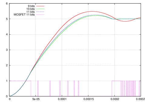
(a) $v_{O}$ from $i_{L}=0,v_{O}=0$

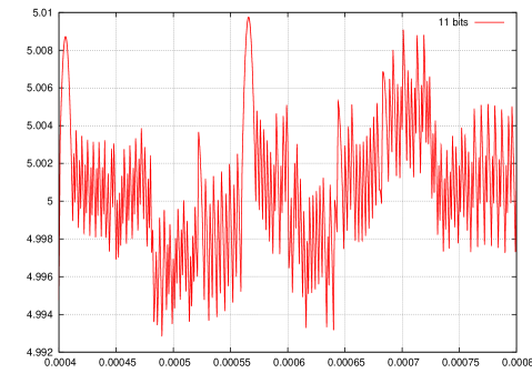
(b) Ripple for $v_{O}$ ($b=11$)

Figure 11: Controller performances for the Buck DC-DC Converter: setup time and ripple.

8.3.2 Setup Time and Ripple

Our model based control software synthesis approach presently does not handle quantitative liveness specifications. Accordingly, quantitative system level formal specifications have to be verified a posteriori. This can be done using a classical Hardware-In-the-Loops (HIL) simulation approach or, even better, following a formal approach, as discussed in [32, 37]. In our context HIL simulation is quite easy since we already have a DTLHS model for the plant and the control software is generated automatically.

To illustrate such a point in this section we highlight HIL simulation results for two quantitative specifications typically considered in control systems: Setup Time and Ripple.

The setup time measures the time it takes to reach the goal (steady state) when the system is turned on. Fig. 11(a) shows trajectories starting from point $(0,0)$ for $K_{9}$, $K_{10}$ and $K_{11}$ as well as the control command sent to the MOSFET (square wave in Fig. 11(a)) for $K_{11}$. Note that all trajectories stabilize (steady state) after only $0.0003$ secs (setup time).

The ripple measures the wideness of the oscillations around the goal (steady state) once this has been reached. Fig. 11(b) shows the ripple for the output voltage after stabilization. For $K_{11}$ we see that the ripple is about $0.01$ V, that is $0.2\%$ of the reference value $V_{\mathrm{ref}}=5$ V.

It is worth noticing that both setup time and ripple compare well with typical figures of commercial high-end buck DC-DC converters (e.g. see [76]) and with the results available from the literature (e.g. [72, 84]).

8.4 Inverted Pendulum: Experimental Settings

Figure 12: Inverted Pendulum with Stationary Pivot Point.

Figure 13: Inverted Pendulum: Controlled region with $b=9$ bits, $F=0.5$, $T=0.1$.

In this section (and in Sects. 8.5, 8.6) we present experiment results obtained by using QKS on the inverted pendulum described in [41], as shown in Fig. 13. The system is modeled by taking the angle $\theta$ and the angular velocity $\dot{\theta}$ as state variables. The input of the system is the torquing force $u$, that can influence the velocity in both directions. Moreover, the behaviour of the system depends on the pendulum mass $m$, the length of the pendulum $l$ and the gravitational acceleration $g$. Given such parameters, the motion of the system is described by the differential equation $\ddot{\theta}={g\over l}\sin\theta+{1\over ml^{2}}u$.

In order to obtain a state space representation, we consider the following normalized system, where $x_{1}$ is the angle $\theta$ and $x_{2}$ is the angular speed $\dot{\theta}$.

$$\dot{x}_{1} = x_{2}$$ (11)

$$\dot{x}_{2} = {g\over l}\sin x_{1}+{1\over ml^{2}}u$$ (12)

Differently from [41], we consider the problem of finding a discrete controller, whose decisions may be “apply the force clockwise” ($u=1$), “apply the force counterclockwise” ($u=-1$), or “do nothing” ($u=0$). The intensity of the force will be given as a constant $F$. Finally, the discrete time transition relation $N$ is obtained from the equations (11-12) as the Euler approximation with sampling time $T$, i.e. the predicate $(x^{\prime}_{1}=x_{1}+Tx_{2})\,\land\,(x^{\prime}_{2}=x_{2}+T{g\over l}\sin x_{1}+T{1\over ml^{2}}Fu)$.

Since the system whose dynamics are in equations (11-12) is not linear, we build a linear over-approximation of it as shown in [3]. The result is the DTLHS ${\cal H}$ defined in Ex. 5 of [3]. From now on we use ${\cal H}$ to denote the inverted pendulum system.

In all our experiments, as in [41], we set parameters $l$ and $m$ in such a way that $\frac{g}{l}=1$ (i.e. $l=g$) and $\frac{1}{ml^{2}}=1$ (i.e. $m=\frac{1}{l^{2}}$). Moreover, we set the force intensity $F=0.5$. More experiments can be found in [3].

As we have done for the buck DC-DC converter, we use uniform quantization functions dividing the domain of each state variable ${\cal D}_{x_{1}}=[-1.1\pi,1.1\pi]$ (we write $\pi$ for a rational approximation of it) and ${\cal D}_{x_{2}}=[-4,4]$ into $2^{b}$ equal intervals, where $b$ is the number of bits used by AD conversion. Since we have two quantized variables, each one with $b$ bits, the number of quantized states is exactly $2^{2b}$.

The typical goal for the inverted pendulum is to turn the pendulum steady to the upright position, starting from any possible initial position, within a given speed interval. In our experiments, the goal region is defined by the predicate $G(X)\equiv(-\rho\leq x_{1}\leq\rho)\,\land\,(-\rho\leq x_{2}\leq\rho)$, where $\rho\in\{0.05,0.1\}$, and the initial region is defined by the predicate $I(X)\equiv(-\pi\leq x_{1}\leq\pi)\,\land\,(-4\leq x_{2}\leq 4$).

We run QKS on the control problem $({\cal H},I,G)$ for different values of the remaining parameters, i.e. $\rho$ (goal tolerance), $T$ (sampling time), and $b$ (number of bits of AD). For each of such experiments, QKS outputs a control software $K$ in C language. In the following, we sometimes make explicit the dependence on $b$ by writing $K_{b}$. In order to evaluate performance of $K$, we use an inverted pendulum simulator written in C. The simulator computes the next state by using Eqs. (11-12), thus simulating a path of ${\cal H}^{(K)}$. Such simulator also introduces random disturbances (up to 4%) in the next state computation to assess $K$ robustness w.r.t. non-modeled disturbances. Finally, in the simulator Eqs. (11-12) are translated into the discrete time version by means of a simulation time step $T_{s}$ much smaller than the sampling time $T$ used in ${\cal H}$. Namely, $T_{s}=10^{-6}$ seconds, whilst $T=0.01$ or $T=0.1$ seconds. This allows us to have a more accurate simulation. Accordingly, $K$ is called each $10^{4}$ (or $10^{5}$) simulation steps of ${\cal H}$. When $K$ is not called, the last chosen action is selected again (sampling and holding).

All experiments for the inverted pendulum have been carried out on an Intel(R) Xeon(R) CPU @ 2.27GHz, with 23GiB of RAM, Debian GNU/Linux 6.0.3 (squeeze).

Table 5: Inverted Pendulum: control abstraction & controller synthesis results with $F=0.5$.

$b$	$T$	$\rho$	$|K|$	CPU	MEM
8	0.1	0.1	2.73e+04	2.56e+03	7.72e+04
9	0.1	0.1	5.94e+04	1.13e+04	1.10e+05
10	0.1	0.1	1.27e+05	5.39e+04	1.97e+05
11	0.01	0.05	4.12e+05	1.47e+05	2.94e+05

8.5 Inverted Pendulum: QKS Performance

To stabilize an underactuated inverted pendulum (i.e. $F<1$) from the hanging position to the upright position, a controller needs to find a non obvious strategy that consists of swinging the pendulum once or more times to gain enough momentum. QKS is able to synthesize such a controller taking as input ${\cal H}$ with $F=0.5$ (note that in [41] $F=0.7$). Results are in Tab. 5, where each row corresponds to a QKS run, columns $b$, $T$ and $\rho$ show the corresponding inverted pendulum parameters, column $|K|$ shows the size of the C code for $K_{b}$, and columns CPU and MEM show the computation time (in seconds) and RAM usage (in KB) needed by QKS to synthesize $K_{b}$.

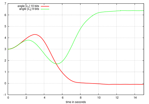
(a) $x_{1}$ from $x_{1}=\pi$, $x_{2}=0$

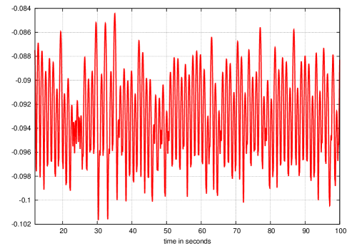
(b) Ripple for $x_{1}$ ($b=10$)

Figure 14: Controller performances for the Inverted Pendulum with $F=0.5$, $b=9,10$: setup time and ripple.

8.6 Inverted Pendulum: Control Software Performance

As for $K_{b}$ performance, it is easy to show that by reducing the sampling time $T$ and the quantization step (i.e. increasing $b$), we increase the quality of $K_{b}$ in terms of ripple and set-up time. Fig. 14(a) shows the simulations of ${\cal H}^{(K_{9})}$ and ${\cal H}^{(K_{10})}$. As we can see, $K_{10}$ drives the system to the goal with a smarter trajectory, with one swing only. This have a significant impact on the set-up time (the system stabilizes after about $8$ seconds when controlled by $K_{10}$ instead of about $10$ seconds required when controlled by $K_{9}$). Fig. 13 shows that the controllable region of $K_{9}$ covers almost all states in the admissible region that we consider. Different colors mean different set of actions enabled by the controller. Finally, Fig. 14(b) shows the ripple of $x_{1}$ for ${\cal H}^{(K_{10})}$ inside the goal. Note that such ripple is very low (0.018 radiants).

9 Related Work

This paper is a journal version of [48] which is extended here by providing omitted proofs and algorithms.

Sect. 9.1 compares our contribution with related work on control software synthesis from system level formal specifications. For the sake of completeness, Sect. 9.2 expands such a comparison to recent results on (non control) software synthesis from formal specifications, focusing on papers using techniques related to ours (constraint solving, OBDD, supervisory control [66]). Sect. 9.3 describes Tab. 6, which summarizes the novelty of our contribution with respect to automatic methods for control software synthesis.

9.1 Control Software Synthesis from System Level Formal Specifications

Control Engineering has been studying control law design (e.g., optimal control, robust control, etc.) for more than half a century (e.g., see [16]). As explained in Sect. 1.1 such results cannot be directly used in our (formal) software synthesis context. On the other hand we note that there are many control systems that are not software based (e.g., in analog circuit design). In such cases, of course, our approach cannot be used.

9.1.1 Control of Linear and Switched Hybrid Systems

The paper closer to our is [41] which studies the problem of control synthesis for discrete time hybrid systems. However, while we present an automatic method, the approach in [41] is not automatic since it requires the user to provide a suitable Lyapunov function (a far from trivial task even for linear hybrid systems).

Quantized Feedback Control has been widely studied in control engineering (e.g. see [26]). However such research addresses linear systems (not the general case of hybrid systems) and focuses on control law design rather than on control software synthesis (our goal). Furthermore, all control engineering approaches model quantization errors as statistical noise. As a result, correctness of the control law holds in a probabilistic sense. Here instead, we model quantization errors as nondeterministic (malicious) disturbances. This guarantees system level correctness of the generated control software (not just that of the control law) with respect to any possible sequence of quantization errors.

Control software synthesis for continuous time linear systems has been widely studied (e.g. see [16]). However such research does not account for quantization. Control software synthesis for continuous time linear systems with quantization has been investigated in [56]. This paper presents an automatic method which, taking as input a continuous time linear system and a goal specification, produces a control law (represented as an OBDD) through Pessoa [55]. While [56] applies to (continuous time) linear systems, our contribution focuses on (discrete time) linear hybrid systems (DTLHSs). Furthermore, although taking into account the quantization process, [56] does not supply an effective method to generate control software (as we do in Sect. 6.1). As a consequence [56] gives no guarantee on WCET, an important issue since an SBCS is a hard real-time system.

[27] presents a method to find an over-approximation of switched systems, under certain stability hypotheses. A switched system is a hybrid system whose mode transitions only depend on control inputs. Such a line of research goes back to [64] which presents a method to compute symbolic models for nonlinear control systems. In combination with [56], such results provide a semi-automatic method for the construction of a control law for switched and nonlinear systems. However, we note that nonlinear systems in [64] are not hybrid systems, since they cannot handle discrete variables. Moreover, while a switched system as in [27] is a linear hybrid system the converse is false since in a linear hybrid system mode transitions can be triggered by state changes (without any change in the input). For example, our approach can synthesize controllers both for the buck DC-DC converter of Fig. 3 (a linear hybrid system) and for the boost DC-DC converter in [27] (a switched system). However, the approach in [27] cannot handle the buck DC-DC converter of Fig. 3 because of the presence of the diode which triggers state dependent mode changes. Moreover, [56] combined with [27] and [64] provide semi-automatic methods since they rely on a Lyapunov function provided by the user, much in the spirit of [41].

9.1.2 Control of Timed Automata and Linear Hybrid Automata

When the plant model is a Timed Automaton (TA) [10, 46] the reachability and control law synthesis problems have both been widely studied. Examples are in [44, 18, 47, 11, 60] and citations thereof. When the plant model is a Linear Hybrid Automaton (LHA) [5, 9] reachability and existence of a control law are both undecidable problems [34, 35]. This, of course, has not prevented devising effective (semi) algorithms for such problems. Examples are in [9, 31, 25, 83, 15]. Much in the same spirit here we give necessary and sufficient constructive conditions for control software existence. Note that none of the above mentioned papers address control software synthesis since they all assume exact (i.e. real valued) state measures (that is, state feedback quantization is not considered).

Continuous-time linear hybrid systems with time delays and given precision of state measurement, Lazy Linear Hybrid Automaton (LLHA), have been studied in [2]. The reachability problem is shown to be undecidable for LLHAs in [1]. Note that such results do not directly apply to our context (Theorem 4.16) since we are addressing discrete-time systems.

9.1.3 Control of Piecewise Affine and Nonlinear Hybrid Systems

Finite horizon control of Piecewise Affine Discrete Time Hybrid Systems (PWA-DTHS) has been studied using a MILP based approach. See, for example, [14]. PWA-DTHSs form a strict subclass of DTLHSs since PWA-DTHS cannot handle linear constraints consisting of discrete state variables whereas DTLHSs can. Such approaches cannot be directly used in our context since they address synthesis of finite horizon controllers and do not account for quantization.

Much in the spirit of [41], [21] presents an explicit control synthesis algorithm for discrete time (possibly nonlinear) hybrid systems, by avoiding the needs of providing Lyapunov functions. Moreover, [22] presents control synthesis algorithms for discrete time hybrid systems cast as universal planning problems. Such approaches cannot be directly used in our context since they do not account for quantization.

Hybrid Toolbox [13] considers continuous time piecewise affine systems. Such a tool outputs a feedback control law that is then passed to Matlab in order to generate control software. We note that such an approach does not account for state feedback quantization and thus, as explained in Sect. 1.1, does not offer any formal guarantee about system level correctness of the generated software, which is instead our focus here.

Using the engine proposed in this paper and computing suitable over-approximations of nonlinear functions, it is possible to address synthesis for nonlinear hybrid systems as done in [3].

9.1.4 Software Synthesis in a Finite Setting

Correct-by-construction software synthesis in a finite state setting has been studied, for example, in [79, 80, 82, 81]. An automatic method for the generation of supervisory controllers for finite state systems is presented in [78]. Control software synthesis in non-deterministic finite domains is studied in [20] (cast as a universal planning problem). Such approaches cannot be directly used in our context since they cannot handle continuous state variables.

In Sect. 6.1 we presented our QFC synthesis algorithm (Alg. 1). Line 3 of Alg. 1 calls function strongCtr (implementing a variant of the algorithm in [20]) in order to compute a time optimal controller for the finite state quantized system. [4] presents a method to obtain a compressed non time optimal controller for a finite state system. This is done by trading the size of the synthesized controller with time optimality while preserving closed loop performances (Remark 6.3). Such a method can be implemented in function strongCtr. Thus, [4] is not an improvement to the present paper but it is a contribution on controller synthesis for finite state systems.

9.1.5 Switching Logic

Optimal switching logic for hybrid systems has been also widely investigated. For example, see [75, 39, 38] and citations thereof. Such approaches, by ignoring the quantization process, indeed focus on the control law design (see Sect. 1.1). However we note that [39, 38] address dwell-time and optimality issues which are not covered by our approach.

9.1.6 Abstraction

Quantization can be seen as a sort of abstraction (the reason for the name control abstraction), which has been widely studied in a hybrid system formal verification context (e.g., see [6, 7, 77, 67]). Note however that in a verification context abstractions are designed so as to ease the verification task whereas in our setting quantization is a design requirement since it models a hardware component (AD converter) which is part of the specification of the control software synthesis problem. Indeed, in our setting, we have to design a controller notwithstanding the nondeterminism stemming from the quantization process. As a result, the techniques used to devise clever abstractions in a verification setting cannot be directly used in our synthesis setting where the quantization to be used is given.

9.2 Software Synthesis from Formal Specifications

Much as control software synthesis, also software synthesis has been widely studied since a long time in many contexts. For examples, see [62, 63, 69, 28]. We give a glimpse of recent results on (non control) software synthesis approaches using techniques related to ours (constraint solving, OBDD, supervisory control).

[12] shows how to mechanically synthesize fault-tolerant concurrent programs for various fault classes. [74] presents a method that synthesizes a program, if there exists one, that meets the input/output specification and uses only the given resources. [29] addresses the problem of synthesizing loop-free programs starting from logical relations between input and output variables. [73] proposes a synthesis technique and applies it to the inversion of imperative programs (e.g., such as insert/delete operations, compressors/decompressors). [19] presents a method for the quantitative, performance-aware synthesis of concurrent programs. Procedures and tools for the automated synthesis of code fragments are also proposed in [43, 30, 42].

Such approaches build on techniques (constraint solving, OBDD, supervisory control) related to ours, but do not address control software synthesis from system level formal specifications.

Table 6: Summary of Related Work. ‘$\bullet$’ stands for ‘Yes’. An empty cell means that feature is not supported.

Citation	T		Input System									K			Impl
	Continuous time	Discrete time	Finite state	Linear	Switched	TA, LHA	Piecewise affine	Linear hybrid sys.	Nonlinear	Nonlinear hybrid sys.	Quantization	Formally verified	Control Software	Guaranteed WCET	Fully automatic	Semi automatic	Tool available
[48] and this paper		$\bullet$		$\bullet$	$\bullet$	$\bullet$	$\bullet$	$\bullet$			$\bullet$	$\bullet$	$\bullet$	$\bullet$	$\bullet$		$\bullet$
[3]		$\bullet$								$\bullet$		$\bullet$	$\bullet$	$\bullet$	$\bullet$		$\bullet$
[4]		$\bullet$	$\bullet$									$\bullet$	$\bullet$	$\bullet$	$\bullet$		$\bullet$
[11]	$\bullet$					$\bullet$						$\bullet$			$\bullet$
[13]	$\bullet$						$\bullet$						$\bullet$		$\bullet$		$\bullet$
[14]		$\bullet$					$\bullet$								$\bullet$
[15]	$\bullet$					$\bullet$						$\bullet$			$\bullet$		$\bullet$
[18]	$\bullet$					$\bullet$						$\bullet$			$\bullet$
[20]		$\bullet$	$\bullet$									$\bullet$	$\bullet$		$\bullet$		$\bullet$
[21]		$\bullet$		$\bullet$	$\bullet$	$\bullet$	$\bullet$	$\bullet$	$\bullet$	$\bullet$					$\bullet$		$\bullet$
[22]		$\bullet$		$\bullet$	$\bullet$	$\bullet$	$\bullet$	$\bullet$							$\bullet$		$\bullet$
[26]	$\bullet$			$\bullet$							$\bullet$
[27]	$\bullet$				$\bullet$						$\bullet$	$\bullet$				$\bullet$
[39]	$\bullet$				$\bullet$							$\bullet$			$\bullet$
[38]	$\bullet$				$\bullet$							$\bullet$			$\bullet$
[41]		$\bullet$		$\bullet$					$\bullet$		$\bullet$	$\bullet$				$\bullet$
[44]	$\bullet$					$\bullet$						$\bullet$			$\bullet$
[47]	$\bullet$					$\bullet$						$\bullet$			$\bullet$
[56]	$\bullet$			$\bullet$							$\bullet$	$\bullet$			$\bullet$		$\bullet$
[60]	$\bullet$					$\bullet$						$\bullet$	$\bullet$		$\bullet$		$\bullet$
[64]	$\bullet$								$\bullet$		$\bullet$	$\bullet$				$\bullet$
[75]	$\bullet$				$\bullet$							$\bullet$			$\bullet$
[78]		$\bullet$	$\bullet$									$\bullet$	$\bullet$		$\bullet$
[79]		$\bullet$	$\bullet$									$\bullet$	$\bullet$		$\bullet$
[80]		$\bullet$	$\bullet$									$\bullet$	$\bullet$		$\bullet$
[82]		$\bullet$	$\bullet$									$\bullet$	$\bullet$		$\bullet$
[81]		$\bullet$	$\bullet$									$\bullet$	$\bullet$		$\bullet$
[83]	$\bullet$					$\bullet$						$\bullet$			$\bullet$

9.3 Summary

Tab. 6 summarizes the novelty of our contribution with respect to automatic methods for control software synthesis (our focus here). For this reason, it only considers papers addressing control software synthesis. Namely, those in Sect. 9.1 but the ones focusing on abstraction (since Sect. 9.2 results do not address control software synthesis).

Tab. 6 is organized as follows. Each row refers to a citation. Each column represents a feature of a cited work. A bullet in a cell means that the citation in the cell row has the feature in the cell column. Where the feature is missing, the cell is empty. The group of columns labeled T denotes whether the input model is expressed in continuous time or discrete time. The group of columns labeled Input System lists the kind of input models we are interested in. Namely: finite state, linear, switched, piecewise affine, TA or LHA, linear hybrid sys., nonlinear, nonlinear hybrid sys. Note that the combination of columns linear hybrid sys. and discrete time denotes our class of DTLHSs. The column labeled Quantization denotes that the row supplies the quantization process. The group of columns labeled K lists the output controller characteristics we are interested in. In particular: Formally verified denotes if the output controller is guaranteed to satisfy the given input specification; Control software indicates if the presented method outputs a control software implementation; Guaranteed WCET denotes if the output controller has a guaranteed WCET. Finally, the group of columns labeled Impl considers implementation issues, namely if a method is fully automatic or semi automatic, and if there exists a tool available implementing the presented method. Note that [27] and [64] in Tab. 6 represent their combination with [56].

Summing up, to the best of our knowledge, no previously published result is available about fully automatic generation (with a tool available) of correct-by-construction control software with a guaranteed WCET from a DTLHS model of the plant, system level formal specifications and implementation specifications (quantization, that is number of bits in AD conversion).

10 Conclusions

We presented an algorithm and a tool QKS implementing it, to support a Formal Model Based Design approach to control software. Our tool takes as input a formal DTLHS model of the plant, implementation specifications (namely, number of bits in AD conversion), and system level formal specifications (namely, safety and liveness properties for the closed loop system). It returns as output a correct-by-construction C implementation (if any) of the control software (namely, Control_Law and Controllable_Region) with a WCET guaranteed to be linear in the number of bits of the quantization schema. We have shown feasibility of our proposed approach by presenting experimental results on using it to synthesize C controllers for the buck DC-DC converter and the inverted pendulum.

In order to speed-up the computation and to avoid possible numerical errors due to MILP solvers [59], a natural possible future research direction is to investigate fully symbolic control software synthesis algorithms based on efficient quantifier elimination procedures (e.g., see [58] and citations thereof).

Acknowledgments

We gratefully acknowledge partial support from FP7 projects GA218815 (ULISSE), 317761 (SmartHG), 600773 (PAEON) and MIUR project DM24283 (TRAMP).

ACRONYMS

AD

Analog-to-Digital

DA

Digital-to-Analog

DTLHS

Discrete Time Linear Hybrid System

DVFS

Dynamic Voltage and Frequency Scaling

HIL

Hardware-In-the-Loop

LHA

Linear Hybrid Automaton

LLHA

Lazy Linear Hybrid Automaton

LTS

Labeled Transition System

MILP

Mixed Integer Linear Programming

OBDD

Ordered Binary Decision Diagram

PWA-DTHS

Piecewise Affine Discrete Time Hybrid Systems

QFC

Quantized Feedback Control

QKS

Quantized feedback Kontrol Synthesizer

SBCS

Software Based Control System

TA

Timed Automaton

WCET

Worst Case Execution Time

Appendix

Appendix A LTS controller synthesis

Symbolic (OBDD based) control software synthesis algorithms for finite state deterministic LTSs have been studied in [80] and citations thereof. In such a context of course strong and weak solutions are the same. Symbolic (OBDD based) control synthesis algorithms for finite state nondeterministic LTSs have been studied in [20] in a universal planning setting. In such a context strong and weak solutions in general differ.

To compute strong solutions, we implemented a variant of the algorithm in [20] in function strongCtr. In our variant, a strong controller for the given LTS control problem is always returned, even if it is not possible to entirely control the given initial region (see Sect. 6.1). More precisely, it returns the strong mgo (see Def. 4.3), i.e. the unique strong solution $K$ to a control problem (${\cal S}$, $I$, $G$) that, disallowing as few actions as possible, drives as many states as possible to a state in $G$ along a shortest path. For the sake of completeness, we show the resulting algorithm in Alg. 4.

Analogously, function existsWeakCtr exploits the algorithm in [80] to verify the existence of weak solutions. Function existsWeakCtr is shown in Alg. 5.

Algorithm 4 Building a strong mgo for an LTS control problem

0.  LTS control problem $({\cal S},I,G)$, with LTS ${\cal S}=(S,A,T)$.

0.  strongCtr(${\cal S},I,G$)

1.  $K(s,a)\leftarrow 0$, $D(s)\leftarrow G(s)$, $\tilde{D}(s)\leftarrow 0$

2.  while $D(s)\neq\tilde{D}(s)$ do

3.     $F(s,a)\leftarrow\exists s^{\prime}:T(s,a,s^{\prime})\land\forall s^{\prime}\;[T(s,a,s^{\prime})\Rightarrow D(s^{\prime})]$

4.     $K(s,a)\leftarrow K(s,a)\lor(F(s,a)\land\not\exists a:K(s,a))$

5.     $\tilde{D}(s)\leftarrow D(s)$, $D(s)\leftarrow D(s)\lor\exists a:K(s,a)$

6.  return $\langle\forall s\;[I(s)\Rightarrow\exists a:K(s,a)],\exists a:K(s,a),K(s,a)\rangle$

Correctness of function strongCtr in Alg. 4 is proved in Prop. A.1.

Proposition A.1.

Let ${\cal S}=(S,A,T)$ be an LTS and ${\cal P}=({\cal S},I,G)$ be an LTS control problem. Then, strongCtr(${\cal S},I,G$) returns $\langle b,D,K\rangle$ s.t. $K$ is the strong mgo for $({\cal S},\varnothing,G)$, $D={\rm Dom}(K)$ and $b$ is True iff $K$ is the strong mgo for ${\cal P}$.

Proof.

We observe that during a generic iteration $i$ the set of states $\{s~{}|~{}\exists a:F(s,a)\}$ is exactly the set of states $F_{i}$ and $\{s~{}|~{}\tilde{D}(s)\}$ is exactly the set of states $D_{i}$ considered in the proof of Prop. 4.18 in Sect. 4.4. As a consequence, the thesis holds by the proof of Prop. 4.18. ∎

Algorithm 5 Existence of weak solutions to LTS control problem

0.  LTS control problem $({\cal S},I,G)$, with LTS ${\cal S}=(S,A,T)$.

0.  existsWeakCtr(${\cal S},I,G$)

1.  $K(s,a)\leftarrow 0$, $D(s)\leftarrow G(s)$, $\tilde{D}(s)\leftarrow 0$

2.  while $D(s)\neq\tilde{D}(s)$ do

3.     $F(s,a)\leftarrow\exists s^{\prime}:[T(s,a,s^{\prime})\land D(s^{\prime})]$

4.     $K(s,a)\leftarrow K(s,a)\lor(F(s,a)\land\not\exists a:K(s,a))$

5.     if $\forall s\;[I(s)\Rightarrow\exists a:K(s,a)]$ then

6.        return  True

7.     $\tilde{D}(s)\leftarrow D(s)$, $D(s)\leftarrow D(s)\lor\exists a:K(s,a)$

8.  return False

Correctness of function existsWeakCtr in Alg. 5 may be proved analogously to Prop. A.1.

Proposition A.2.

Let ${\cal S}=(S,A,T)$ be an LTS and ${\cal P}=({\cal S},I,G)$ be an LTS control problem. Then, existsWeakCtr(${\cal S},I,G$) returns True iff there exists a weak mgo for ${\cal P}$.

Corollary A.3.

Let ${\cal S}=(S,A,T)$ be an LTS and ${\cal P}=({\cal S},I,G)$ be an LTS control problem. Then, existsWeakCtr(${\cal S},I,G$) returns True iff there exists a weak solution for ${\cal P}$.

Appendix B Details about the Experiments

In this section we give (Tab. 7) all details about MILP problems arising in our experiments about the buck DC/DC converter of Sects. 8.1–8.3. Namely, in Tab. 7 MILP$i$ has the same meaning as in Sect. 8.2.1, i.e. MILP1 refers to the MILP problems described in Sect. 6.3, i.e. those computing the quantization for $I$ and $G$, MILP2 refers to MILP problems in function SelfLoop (see Alg. 3), MILP3 refers to the MILP problems used in function overImg (line 6 of Alg. 2), MILP4 refers to MILP problems used to check actions admissibility (line 8 of Alg. 2), and MILP5 refers to MILP problems used to check transitions witnesses (line 4 of Alg. 2). In Tab. 7 columns $b$, Num, Avg and Tot are the same as columns $b$, Num, Avg and Time of Tabs. 3 and 4 thus $b$ shows the number of AD bits, Num is the number of times that the MILP problem of the given type is called, Tot is the total CPU time needed to solve all the Num instances of MILP problem of the given type, and Avg is the ratio between Tot and Num. In Tab. 7 we also show in columns Min and Max the average, minimum and maximum time to solve one MILP problem of the given type. The standard deviation for such statistics is given in column DevStd.

Table 7: Complete statistics for Tabs. 3 and 4 of Sect. 8.

MILP1
$b$	Num	Tot	Avg	Min	Max	DevStd
8	6.55e+04	4.61e+00	7.03e-05	0.00e+00	1.00e-02	8.35e-04
9	2.62e+05	1.84e+01	7.02e-05	0.00e+00	1.00e-02	8.35e-04
10	1.05e+06	2.79e+02	2.66e-04	0.00e+00	1.00e-02	1.61e-03
11	4.19e+06	9.65e+02	2.30e-04	0.00e+00	1.00e-02	1.50e-03
MILP2
$b$	Num	Tot	Avg	Min	Max	DevStd
8	3.99e+05	3.25e+02	1.52e-03	0.00e+00	1.00e-02	4.39e-03
9	1.59e+06	1.12e+03	1.41e-03	0.00e+00	1.00e-02	4.14e-03
10	6.36e+06	1.35e+04	3.78e-03	0.00e+00	1.00e-02	6.43e-03
11	2.54e+07	4.56e+04	3.26e-03	0.00e+00	1.00e-02	6.10e-03
MILP3
$b$	Num	Tot	Avg	Min	Max	DevStd
8	2.31e+05	2.10e+02	9.10e-04	0.00e+00	1.00e-02	3.20e-03
9	9.21e+05	8.44e+02	9.16e-04	0.00e+00	1.00e-02	3.18e-03
10	3.68e+06	1.11e+04	3.00e-03	0.00e+00	2.00e-02	4.26e-03
11	1.47e+07	3.76e+04	2.55e-03	0.00e+00	2.00e-02	4.02e-03
MILP4
$b$	Num	Tot	Avg	Min	Max	DevStd
8	7.80e+05	7.71e+02	9.89e-04	0.00e+00	1.00e-02	2.98e-03
9	4.42e+06	4.49e+03	1.02e-03	0.00e+00	1.00e-02	3.02e-03
10	3.01e+07	7.75e+04	2.58e-03	0.00e+00	2.00e-02	4.37e-03
11	2.61e+08	5.66e+05	2.17e-03	0.00e+00	2.00e-02	4.13e-03
MILP5
$b$	Num	Tot	Avg	Min	Max	DevStd
8	4.27e+05	1.20e+02	2.80e-04	0.00e+00	1.00e-02	1.65e-03
9	1.71e+06	4.87e+02	2.85e-04	0.00e+00	1.00e-02	1.66e-03
10	6.84e+06	1.25e+04	1.83e-03	0.00e+00	2.00e-02	3.87e-03
11	2.74e+07	4.25e+04	1.55e-03	0.00e+00	2.00e-02	3.62e-03

References

- [1] Manindra Agrawal, Frank Stephan, P. S. Thiagarajan, and Shaofa Yang. Behavioural approximations for restricted linear differential hybrid automata. In João P. Hespanha and Ashish Tiwari, editors, Proceedings of Hybrid Systems: Computation and Control, 9th International Workshop, HSCC, volume 3927 of Lecture Notes in Computer Science, pages 4–18. Springer, 2006.
- [2] Manindra Agrawal and P. S. Thiagarajan. The discrete time behavior of lazy linear hybrid automata. In Manfred Morari and Lothar Thiele, editors, Proceedings of Hybrid Systems: Computation and Control, 8th International Workshop, HSCC, volume 3414 of Lecture Notes in Computer Science, pages 55–69. Springer, 2005.
- [3] Vadim Alimguzhin, Federico Mari, Igor Melatti, Ivano Salvo, and Enrico Tronci. Automatic control software synthesis for quantized discrete time hybrid systems. In Conference on Decision and Control, CDC, 2012. To Appear. A preliminary version can be found at http://arxiv.org/abs/1207.4098.
- [4] Vadim Alimguzhin, Federico Mari, Igor Melatti, Ivano Salvo, and Enrico Tronci. On model based synthesis of embedded control software. In International Conference on Embedded Software, EMSOFT, 2012. To Appear. A preliminary version can be found at arxiv.org.
- [5] R. Alur, C. Courcoubetis, N. Halbwachs, T. A. Henzinger, P. H. Ho, X. Nicollin, A. Olivero, J. Sifakis, and S. Yovine. The algorithmic analysis of hybrid systems. Theoretical Computer Science, 138(1):3 – 34, 1995.
- [6] R. Alur, T.A. Henzinger, G. Lafferriere, and G.J. Pappas. Discrete abstractions of hybrid systems. Proceedings of the IEEE, 88(7):971–984, 2000.
- [7] Rajeev Alur, Thao Dang, and Franjo Ivančić. Predicate abstraction for reachability analysis of hybrid systems. ACM Trans. on Embedded Computing Sys., 5(1):152–199, 2006.
- [8] Rajeev Alur and David L. Dill. A theory of timed automata. Theor. Comput. Sci., 126:183–235, April 1994.
- [9] Rajeev Alur, Thomas A. Henzinger, and Pei-Hsin Ho. Automatic symbolic verification of embedded systems. IEEE Trans. Softw. Eng., 22(3):181–201, 1996.
- [10] Rajeev Alur and P. Madhusudan. Decision problems for timed automata: A survey. In SFM, LNCS 3185, pages 1–24, 2004.
- [11] Eugene Asarin and Oded Maler. As soon as possible: Time optimal control for timed automata. In HSCC, LNCS 1569, pages 19–30, 1999.
- [12] Paul C. Attie, Anish Arora, and E. Allen Emerson. Synthesis of fault-tolerant concurrent programs. ACM Transactions on Programming Languages Systems (TOPLAS), 26(1):125–185, 2004.
- [13] A. Bemporad. Hybrid Toolbox, 2004. http://cse.lab.imtlucca.it/~bemporad/hybrid/toolbox/.
- [14] Alberto Bemporad and Nicolò Giorgetti. A sat-based hybrid solver for optimal control of hybrid systems. In HSCC, LNCS 2993, pages 126–141, 2004.
- [15] Massimo Benerecetti, Marco Faella, and Stefano Minopoli. Revisiting synthesis of switching controllers for linear hybrid systems. In Decision and Control and European Control Conference (CDC-ECC), 2011 50th IEEE Conference on, pages 4753 –4758, dec. 2011.
- [16] William L. Brogan. Modern control theory (3rd ed.). Prentice-Hall, Inc., Upper Saddle River, NJ, USA, 1991.
- [17] R. Bryant. Graph-based algorithms for boolean function manipulation. IEEE Trans. on Computers, C-35(8):677–691, 1986.
- [18] Franck Cassez, Alexandre David, Emmanuel Fleury, Kim Guldstrand Larsen, and Didier Lime. Efficient on-the-fly algorithms for the analysis of timed games. In CONCUR, LNCS 3653, pages 66–80, 2005.
- [19] Pavol Cerný, Krishnendu Chatterjee, Thomas A. Henzinger, Arjun Radhakrishna, and Rohit Singh. Quantitative synthesis for concurrent programs. In Ganesh Gopalakrishnan and Shaz Qadeer, editors, Computer Aided Verification, pages 243–259. Springer, 2011.
- [20] Alessandro Cimatti, Marco Roveri, and Paolo Traverso. Strong planning in non-deterministic domains via model checking. In AIPS, pages 36–43, 1998.
- [21] G. Della Penna, D. Magazzeni, A. Tofani, B. Intrigila, I. Melatti, and E. Tronci. Automated Generation of Optimal Controllers through Model Checking Techniques, volume 15 of Lecture Notes in Electrical Engineering. Springer, 2008.
- [22] Giuseppe Della Penna, Daniele Magazzeni, Fabio Mercorio, and Benedetto Intrigila. UPMurphi: A tool for universal planning on pddl+ problems. In ICAPS, 2009.
- [23] A.D. Dominguez-Garcia and P.T. Krein. Integrating reliability into the design of fault-tolerant power electronics systems. In PESC, pages 2665–2671. IEEE, 2008.
- [24] Johan Eker, Jorn Janneck, Edward A. Lee, Jie Liu, Xiaojun Liu, Jozsef Ludvig, Sonia Sachs, and Yuhong Xiong. Taming heterogeneity - the ptolemy approach. Proceedings of the IEEE, 91(1):127–144, January 2003.
- [25] Goran Frehse. Phaver: algorithmic verification of hybrid systems past hytech. Int. J. Softw. Tools Technol. Transf., 10(3):263–279, 2008.
- [26] Minyue Fu and Lihua Xie. The sector bound approach to quantized feedback control. IEEE Trans. on Automatic Control, 50(11):1698–1711, 2005.
- [27] A. Girard, G. Pola, and P. Tabuada. Approximately bisimilar symbolic models for incrementally stable switched systems. IEEE Transactions on Automatic Control, 55(1):116–126, 2010.
- [28] Alain Girault and Éric Rutten. Automating the addition of fault tolerance with discrete controller synthesis. Formal Methods in System Design, 35(2):190–225, 2009.
- [29] Sumit Gulwani, Susmit Jha, Ashish Tiwari, and Ramarathnam Venkatesan. Synthesis of loop-free programs. In Mary W. Hall and David A. Padua, editors, 32nd Conference on Programming Language Design and Implementation, PLDI, pages 62–73. ACM, 2011.
- [30] Tihomir Gvero, Viktor Kuncak, and Ruzica Piskac. Interactive synthesis of code snippets. In Ganesh Gopalakrishnan and Shaz Qadeer, editors, Computer Aided Verification - 23rd International Conference, CAV, volume 6806 of Lecture Notes in Computer Science, pages 418–423. Springer, 2011.
- [31] T.A. Henzinger, P.-H. Ho, and H. Wong-Toi. Hytech: A model checker for hybrid systems. STTT, 1(1):110–122, 1997.
- [32] Thomas A. Henzinger. From boolean to quantitative notions of correctness. In POPL, pages 157–158. ACM, 2010.
- [33] Thomas A. Henzinger, Benjamin Horowitz, Rupak Majumdar, and Howard Wong-Toi. Beyond hytech: Hybrid systems analysis using interval numerical methods. In HSCC, LNCS 1790, pages 130–144, 2000.
- [34] Thomas A. Henzinger and Peter W. Kopke. Discrete-time control for rectangular hybrid automata. In ICALP, pages 582–593, 1997.
- [35] Thomas A. Henzinger, Peter W. Kopke, Anuj Puri, and Pravin Varaiya. What’s decidable about hybrid automata? J. of Computer and System Sciences, 57(1):94–124, 1998.
- [36] Thomas A. Henzinger and Joseph Sifakis. The embedded systems design challenge. In FM, LNCS 4085, pages 1–15, 2006.
- [37] Holger Hermanns, Kim Guldstrand Larsen, Jean-François Raskin, and Jan Tretmans. Quantitative system validation in model driven design. In EMSOFT, pages 301–302. ACM, 2010.
- [38] Susmit Jha, Sanjit A. Seshia, and Ashish Tiwari. Synthesis of optimal switching logic for hybrid systems. In EMSOFT, pages 107–116. ACM, 2011.
- [39] Susmit Kumar Jha, Sumit Gulwani, Sanjit A. Seshia, and Ashish Tiwari. Synthesizing switching logic for safety and dwell-time requirements. Technical Report UCB/EECS-2010-28, EECS Department, University of California, Berkeley, Mar 2010.
- [40] W. Kim, M. S. Gupta, G.-Y. Wei, and D. M. Brooks. Enabling on-chip switching regulators for multi-core processors using current staggering. In ASGI, 2007.
- [41] Gerhard Kreisselmeier and Thomas Birkhölzer. Numerical nonlinear regulator design. IEEE Trans. on on Automatic Control, 39(1):33–46, 1994.
- [42] Viktor Kuncak, Mikaël Mayer, Ruzica Piskac, and Philippe Suter. Comfusy: A tool for complete functional synthesis. In Tayssir Touili, Byron Cook, and Paul Jackson, editors, Computer Aided Verification, 22nd International Conference, CAV, volume 6174 of Lecture Notes in Computer Science, pages 430–433. Springer, 2010.
- [43] Viktor Kuncak, Mikaël Mayer, Ruzica Piskac, and Philippe Suter. Software synthesis procedures. Commun. ACM, 55(2):103–111, 2012.
- [44] Kim Guldstrand Larsen, Paul Pettersson, and Wang Yi. Uppaal: Status & developments. In CAV, LNCS 1254, pages 456–459, 1997.
- [45] Ping-Zong Lin, Chun-Fei Hsu, and Tsu-Tian Lee. Type-2 fuzzy logic controller design for buck dc-dc converters. In FUZZ, pages 365–370, 2005.
- [46] Oded Maler, Zohar Manna, and Amir Pnueli. From timed to hybrid systems. In J. W. de Bakker, Cornelis Huizing, Willem P. de Roever, and Grzegorz Rozenberg, editors, Proceedings of Real-Time: Theory in Practice, REX Workshop, volume 600 of Lecture Notes in Computer Science, pages 447–484. Springer, 1992.
- [47] Oded Maler, Dejan Nickovic, and Amir Pnueli. On synthesizing controllers from bounded-response properties. In CAV, LNCS 4590, pages 95–107. Springer, 2007.
- [48] Federico Mari, Igor Melatti, Ivano Salvo, and Enrico Tronci. Synthesis of quantized feedback control software for discrete time linear hybrid systems. In CAV, LNCS 6174, pages 180–195, 2010.
- [49] Federico Mari, Igor Melatti, Ivano Salvo, and Enrico Tronci. From boolean relations to control software. In ICSEA, 2011.
- [50] Federico Mari, Igor Melatti, Ivano Salvo, and Enrico Tronci. Quantized feedback control software synthesis from system level formal specifications. CoRR, abs/1107.5638v1, 2011.
- [51] Federico Mari, Igor Melatti, Ivano Salvo, and Enrico Tronci. Quantized feedback control software synthesis from system level formal specifications for buck dc/dc converters. CoRR, abs/1105.5640, 2011.
- [52] Federico Mari, Igor Melatti, Ivano Salvo, and Enrico Tronci. Control software visualization. In Proceedings of INFOCOMP 2012, The Second International Conference on Advanced Communications and Computation, pages 15–20. ThinkMind, 2012.
- [53] Federico Mari, Igor Melatti, Ivano Salvo, and Enrico Tronci. Linear constraints as a modeling language for discrete time hybrid systems. In Proceedings of ICSEA 2012, The Seventh International Conference on Software Engineering Advances, pages 664–671. ThinkMind, 2012.
- [54] Federico Mari, Igor Melatti, Ivano Salvo, and Enrico Tronci. Undecidability of quantized state feedback control for discrete time linear hybrid systems. In A. Roychoudhury and M. D’Souza, editors, Proceedings of the International Colloquium on Theoretical Aspects of Computing, ICTAC, volume 7521 of LNCS, pages 243–258. Springer-Verlag Berlin Heidelberg, 2012.
- [55] Manuel Mazo, Anna Davitian, and Paulo Tabuada. Pessoa: A tool for embedded controller synthesis. In CAV, LNCS 6174, pages 566–569, 2010.
- [56] Manuel Jr Mazo and Paulo Tabuada. Symbolic approximate time-optimal control. Systems & Control Letters, 60(4):256–263, 2011.
- [57] Marvin L. Minsky. Recursive unsolvability of post’s problem of ”tag” and other topics in theory of turing machines. The Annals of Mathematics, 74(3):pp. 437–455, 1961.
- [58] David Monniaux. Quantifier elimination by lazy model enumeration. In CAV, LNCS 6174, pages 585–599, 2010.
- [59] A. Neumaier and O. Shcherbina. Safe bounds in linear and mixed-integer programming. Mathematical Programming, Ser. A, 99:283–296, 2004.
- [60] Hans-Jörg Peter, Rüdiger Ehlers, and Robert Mattmüller. Synthia: Verification and synthesis for timed automata. In Ganesh Gopalakrishnan and Shaz Qadeer, editors, Computer Aided Verification, pages 649–655. Springer, 2011.
- [61] André Platzer and Edmund M. Clarke. Formal verification of curved flight collision avoidance maneuvers: A case study. In Ana Cavalcanti and Dennis Dams, editors, Proceedings of FM 2009: Formal Methods, Second World Congress, volume 5850 of Lecture Notes in Computer Science, pages 547–562. Springer, 2009.
- [62] Amir Pnueli and Roni Rosner. On the synthesis of a reactive module. In Conference Record of the Sixteenth Annual ACM Symposium on Principles of Programming Languages, POPL, pages 179–190. ACM Press, 1989.
- [63] Amir Pnueli and Roni Rosner. On the synthesis of an asynchronous reactive module. In Giorgio Ausiello, Mariangiola Dezani-Ciancaglini, and Simona Ronchi Della Rocca, editors, Automata, Languages and Programming, 16th International Colloquium, ICALP, volume 372 of Lecture Notes in Computer Science, pages 652–671. Springer, 1989.
- [64] G. Pola, A. Girard, and P. Tabuada. Symbolic models for nonlinear control systems using approximate bisimulation. In Decision and Control, 2007 46th IEEE Conference on, pages 4656 –4661, dec. 2007.
- [65] http://mclab.di.uniroma1.it/, 2011.
- [66] P. J. Ramadge and W. M. Wonham. Supervisory control of a class of discrete event processes. SIAM Journal Control Optimization, 25(1):206–230, jan 1987.
- [67] Sriram Sankaranarayanan and Ashish Tiwari. Relational abstractions for continuous and hybrid systems. In Ganesh Gopalakrishnan and Shaz Qadeer, editors, Computer Aided Verification, pages 686–702. Springer, 2011.
- [68] http://www.esterel-technologies.com/products/scade-system/, 2012.
- [69] Sven Schewe and Bernd Finkbeiner. Synthesis of asynchronous systems. In Germán Puebla, editor, Logic-Based Program Synthesis and Transformation, 16th International Symposium, LOPSTR, volume 4407 of Lecture Notes in Computer Science, pages 127–142. Springer, 2006.
- [70] G. Schrom, P. Hazucha, J. Hahn, D.S. Gardner, B.A. Bloechel, G. Dermer, S.G. Narendra, T. Karnik, and V. De. A 480-mhz, multi-phase interleaved buck dc-dc converter with hysteretic control. In PESC, pages 4702–4707 vol. 6. IEEE, 2004.
- [71] http://www.mathworks.it/products/simulink/, 2012.
- [72] Wing-Chi So, C.K. Tse, and Yim-Shu Lee. Development of a fuzzy logic controller for dc/dc converters: design, computer simulation, and experimental evaluation. IEEE Trans. on Power Electronics, 11(1):24–32, 1996.
- [73] Saurabh Srivastava, Sumit Gulwani, Swarat Chaudhuri, and Jeffrey S. Foster. Path-based inductive synthesis for program inversion. In Mary W. Hall and David A. Padua, editors, 32nd Conference on Programming Language Design and Implementation, PLDI, pages 492–503. ACM, 2011.
- [74] Saurabh Srivastava, Sumit Gulwani, and Jeffrey S. Foster. From program verification to program synthesis. In Manuel V. Hermenegildo and Jens Palsberg, editors, 37th Symposium on Principles of Programming Languages, POPL, pages 313–326. ACM, 2010.
- [75] A. Taly, S. Gulwani, and A. Tiwari. Synthesizing switching logic using constraint solving. In Proc. 10th Intl. Conf. on Verification, Model Checking and Abstract Interpretation, VMCAI, volume 5403 of LNCS, pages 305–319. Springer, 2009.
- [76] Slvp182: High accuracy synchronous buck dc-dc converter: http://focus.ti.com.cn/cn/lit/ug/slvu046/slvu046.pdf, 2001.
- [77] Ashish Tiwari. Abstractions for hybrid systems. In Formal Methods in Systems Design, 2008.
- [78] Enrico Tronci. Optimal finite state supervisory control. In CDC. IEEE, 1996.
- [79] Enrico Tronci. On computing optimal controllers for finite state systems. In CDC, pages 3592–3593 vol. 4. IEEE, 1997.
- [80] Enrico Tronci. Automatic synthesis of controllers from formal specifications. In ICFEM, pages 134–143. IEEE, 1998.
- [81] Enrico Tronci. Automatic synthesis of control software for an industrial automation control system. In ASE, pages 247–250. IEEE, 1999.
- [82] Enrico Tronci. Formally modeling a metal processing plant and its closed loop specifications. In HASE, page 151. IEEE, 1999.
- [83] H. Wong-Toi. The synthesis of controllers for linear hybrid automata. In CDC, pages 4607–4612 vol. 5. IEEE, 1997.
- [84] V. Yousefzadeh, A. Babazadeh, B. Ramachandran, E. Alarcon, L. Pao, and D. Maksimovic. Proximate time-optimal digital control for synchronous buck dc–dc converters. IEEE Trans. on Power Electronics, 23(4):2018–2026, 2008.