Exploring Spiral Defect Chaos in Generalized Swift-Hohenberg Models with Mean Flow

Abstract

We explore the phenomenon of spiral defect chaos in two types of generalized Swift-Hohenberg model equations that include the effects of long-range drift velocity or mean flow. We use spatially-extended domains and integrate the equations for very long times to study the pattern dynamics as the magnitude of the mean flow is varied. The magnitude of the mean flow is adjusted via a real and continuous parameter that accounts for the fluid boundary conditions on the horizontal surfaces in a convecting layer. For weak values of the mean flow we find that the patterns exhibit a slow coarsening to a state dominated by large and very slowly moving target defects. For strong enough mean flow we identify the existence of spatiotemporal chaos which is indicated by a positive leading order Lyapunov exponent. We compare the spatial features of the mean flow field with that of Rayleigh-Bénard convection and quantify their differences in the neighborhood of spiral defects.

I Introduction

The chaotic behavior of spatially-extended dissipative systems has been intensively studied in recent years Cross and Hohenberg (1993). Spatiotemporal chaos has been observed in a wide range of physical systems including Faraday waves that appear on the surface of an oscillating layer of fluid Gollub and Ramshankar (1991), reacting chemical mixtures Skinner and Swinney (1991), excitable media Bar and Eiswirth (1993), and Rayleigh-Bénard convection in a shallow fluid layer heated from below Cross and Hohenberg (1993). In particular, the study of Rayleigh-Bénard convection continues to provide fundamental insights into the dynamics of pattern forming systems that are driven far-from-equilibrium Cross and Hohenberg (1993); Bodenschatz et al. (2000). The state of spiral defect chaos has received significant attention since its discovery by Morris et al. Morris et al. (1993). Spiral defect chaos is characterized by the complex dynamics of rotating spiral defects and interestingly, occurs for fluid parameters where straight parallel convection rolls are linearly stable Cross and Hohenberg (1993); Bodenschatz et al. (2000). Although much effort has been spent on building our understanding of the origins and dynamical features of spiral defect chaos, many open questions still remain.

A significant difficulty in studying spatiotemporal chaos is that the experimental systems of interest are often large and strongly driven. This presents significant obstacles for both analytical and numerical approaches. For example, the numerical simulation of the Boussinesq equations, which govern Rayleigh-Bénard convection, in large domains, for long simulation times, and for many values of the system parameters is out of reach using currently available algorithms and computing resources. Although significant progress has been made in the ability to simulate convection for experimental conditions, the computational cost remains very high Paul et al. (2003). In light of challenges such as these, the use of simpler model equations has played a pivotal role in furthering our physical understanding of spatiotemporal chaos. In Rayleigh-Bénard convection, the two-dimensional Swift-Hohenberg equation Swift and Hohenberg (1977) has led to numerous physical insights regarding questions of pattern formation Cross and Hohenberg (1993). However, the use of the Swift-Hohenberg equation to study spatiotemporal chaos, and in particular spiral defect chaos Xi et al. (1993), has been called into question Schmitz et al. (2002), as will be further discussed below. This leaves no clear choice for a model system to be used for the study of spiral defect chaos with direct relevance to fluid convection.

The presence of a long-range mean flow is well known to play an important role in the dynamics of Rayleigh-Bénard convection Cross and Hohenberg (1993); Newell et al. (1990a, b). This led to extensions of the Swift-Hohenberg equation to account for these effects Manneville (1984); Cross and Tu (1995); Xi et al. (1993). The mean flow is a weak horizontal flow field that acts over length scales larger than that of the convection rolls; it results from the coupling to fluid vertical vorticity and is induced by roll curvature, amplitude gradients, and wavenumber gradients Siggia and Zippelius (1981); Manneville (1983); Cross and Hohenberg (1993). The magnitude of the mean flow is much smaller than that of the convective roll motion, making it very difficult to measure in experiment. A typical way to visualize the mean flow in numerical work is to present contours of the integrated horizontal components of the fluid velocity over the depth of the fluid layer Paul et al. (2003). Although the mean flow is weak it can have significant effect upon the dynamics and stability boundaries of the flow field and also adds a slow time scale to the dynamics. It has been shown numerically that the mean flow is required for spiral defect chaos in Rayleigh-Bénard convection Chiam et al. (2003).

Spiral defect chaos was initially explored using numerical simulations of the generalized Swift-Hohenberg equation by Xi et al. Xi et al. (1993). These simulations were for rather short intervals of time $t\sim 900$ where $t$ is the nondimensional time. We note that to generate the spiral defect state in this model system, the system needs to be taken far enough from the convective threshold; otherwise roll-type patterns would dominate with the system dynamics governed by the motion of topological defects such as grain boundaries, dislocations, and disclinations Huang and Viñals (2007). Schmitz et al. Schmitz et al. (2002) later explored the generalized Swift-Hohenberg equation for the same parameters but for much longer simulation times $t\sim 64000$. Their results suggested that the spiral defect state was only a transient with the long-time dynamics characterized by a slow coarsening process to a state dominated by large spirals. This work has cast doubt upon the ability of the Swift-Hohenberg equation to exhibit persistent dynamics that resemble spiral defect chaos.

In this paper, we present a careful numerical study of these questions. In particular, we have performed very long-time simulations ($t=10^{6}$ time units) in very large domains, and for a wide range of mean flow strengths. We also compute the leading order Lyapunov exponent to determine if the dynamics are chaotic. Our investigation is driven by the results on Rayleigh-Bénard convection that demonstrate the importance of mean flow upon spiral defect chaos Paul et al. (2003); Bodenschatz et al. (2000).

The remainder of this paper is organized as follows. In Sec. II we discuss two types of generalized Swift-Hohenberg model equations and provide some details regarding its numerical solution and the computation of the leading order Lyapunov exponent. In Sec. III we present our results and discuss the role of the mean flow upon the dynamics. Concluding remarks are given in Sec. IV.

II Approach

II.1 The Generalized Swift-Hohenberg Models

A generalized, dimensionless form of the two-dimensional time-dependent Swift-Hohenberg model is given by Xi et al. (1993)

$$\frac{\partial\psi}{\partial t}+\mathbf{U}\cdot\nabla\psi=\epsilon\psi-(\nabla^{2}+1)^{2}\psi+N[\psi],$$ (1)

$$\left[\frac{\partial}{\partial t}-\sigma\left(\nabla^{2}-c^{2}\right)\right]\nabla^{2}\zeta=g_{m}\left[\nabla\left(\nabla^{2}\psi\right)\times\nabla\psi\right]\cdot\hat{\mathbf{z}},$$ (2)

where $\psi(x,y,t)$ is a scalar field describing the spatial and temporal variation of the convection patterns, $\epsilon$ is a control parameter giving the dimensionless distance from the convective threshold, and $\hat{\mathbf{z}}$ represents the unit vector in the out-of-plane direction. The variable $\zeta(x,y,t)$ is the vertical vorticity potential defined via $\Omega_{z}=(\nabla\times\mathbf{U})_{z}=-\nabla^{2}\zeta$, where $\Omega_{z}$ is the vertical component of fluid vorticity and $\mathbf{U}$ is the mean flow or drift velocity. $\zeta$ can also be interpreted as the stream function for the mean flow, given that

$$\mathbf{U}=\nabla\times\left(\zeta\hat{\mathbf{z}}\right)=\left(\partial_{y}\zeta,-\partial_{x}\zeta\right).$$ (3)

In Eq. (2) $\sigma$ is proportional to the Prandtl number, $g_{m}$ is a positive real constant that characterizes the mean flow coupling strength, and $c$ is a real parameter introduced for modeling the effect of free-slip ($c=0$) or no-slip ($c\neq 0$) boundary conditions for the horizontal surfaces of a convection layer. The term $N[\psi]$ in Eq. (1) represents the nonlinearity of the system, which has many different forms in the literature based on system conditions Greenside and Cross (1985); Cross and Hohenberg (1993); Manneville (1984). In this paper we present numerical results for two representative cases: (1) $N[\psi]=-\psi^{3}$ for which the model equations are referred to as the Generalized Swift-Hohenberg (GSH) model Greenside and Cross (1985), and (2) $N[\psi]=-(|\nabla\psi|^{2}\psi+\psi^{3})$ for which the equations are referred to as Manneville’s model that was derived in Refs. Manneville (1983, 1984) from the Boussinesq equations.

II.2 Numerical Simulations

We numerically integrate Eqs. (1)–(2) using the approach discussed by Cross et al. Cross et al. (1994) and provide only the essential details here. The domain is a square geometry that is discretized on a spatially uniform grid with periodic lateral boundary conditions. In our numerical simulations we begin from random initial conditions for $\psi$ and set initially $\zeta(x,y,t=0)=0$. We discretize the spatial domain using a $512\times 512$ grid with a grid spacing of $\Delta x=\Delta y=\lambda_{0}/8$ where $\lambda_{0}=2\pi$ is the critical wavelength of a convection roll. These parameters are approximately equivalent to a Rayleigh-Bénard system in a box geometry with an aspect ratio of $\Gamma=L/d=128$ where $L$ is the side length of the box and $d$ is the depth of the convection layer. Each individual simulation is allowed to evolve for $t=10^{6}$ time units using a time step of $\Delta t=0.2$.

The equations are stiff due to the very fast dynamics of the biharmonic operator in comparison to the much slower convective time scale of the pattern dynamics. An efficient solution is obtained using a pseudospectral operator-splitting approach Canuto et al. (1988). The linear terms are treated exactly using an explicit exponential time integration Cox and Matthews (2002); Kassam and Trefethen (2005) and the nonlinear terms are evolved forward in time using an explicit predictor-corrector approach. To reduce the contributions of high wavenumber modes in the vorticity field a Gaussian filtering operator $F_{\gamma}$ is applied to the right-hand side of Eq. (2) Greenside and Cross (1985). In Fourier space it is given by $F_{\gamma}=\exp\left(-{\gamma}^{2}q^{2}/2\right)$ where $\gamma$ is the filtering radius and $q$ is the wavenumber. In our simulations we have used a filtering radius of $\gamma=\lambda_{0}/2$.

We compute the leading order Lyapunov exponent using the standard procedure described in detail in Ref. Wolf et al. (1985). The tangent space equations are,

$$\frac{\partial\delta\psi}{\partial t}+\mathbf{U}\cdot\nabla\delta\psi+\delta\mathbf{U}\cdot\nabla\psi=\epsilon\delta\psi-(\nabla^{2}+1)^{2}\delta\psi$$

$$+\delta N[\psi,\delta\psi],$$ (4)

$$\left[\frac{\partial}{\partial t}-\sigma\left(\nabla^{2}-c^{2}\right)\right]\nabla^{2}\delta\zeta=g_{m}\left[\nabla\left(\nabla^{2}\delta\psi\right)\times\nabla\psi\right.$$

$$+\left.\nabla\left(\nabla^{2}\psi\right)\times\nabla\delta\psi\right]\cdot\hat{\mathbf{z}},$$ (5)

where $\delta\mathbf{U}=\nabla\times\left(\delta\zeta\hat{\mathbf{z}}\right)$. The nonlinear term for the GSH equation is

$$\delta N[\psi,\delta\psi]=-3\psi^{2}\delta\psi,$$ (6)

and for Manneville’s model it is

$$\delta N[\psi,\delta\psi]=-\left(3\psi^{2}+|\nabla\psi|^{2}\right)\delta\psi-2\left[(\nabla\psi)\cdot(\nabla\delta\psi)\right]\psi.$$ (7)

The magnitude of $\delta\psi$ is renormalized after a time $t_{N}$ to yield a measure of its growth $\|\delta\psi(t_{N})\|$ which is used to calculate the instantaneous Lyapunov exponent, i.e.,

$$\tilde{\lambda}_{1}=\frac{1}{t_{N}}\ln\|\delta\psi(t_{N})\|.$$ (8)

We have used $t_{N}=2$ in our simulations. This normalization is repeated in time to generate many values of the instantaneous Lyapunov exponent whose time average yields the finite-time Lyapunov exponent

$$\lambda_{1}=\frac{1}{N_{t}}\sum_{i=1}^{N_{t}}\tilde{\lambda}_{1}$$ (9)

where $N_{t}$ is the number of renormalizations performed. The limit $N_{t}\rightarrow\infty$ yields the infinite-time Lyapunov exponent.

III Results

Experimental measurements of spiral defect chaos have typically been performed using large aspect ratio domains, moderate Rayleigh numbers, and compressed gases with Prandtl number of approximately unity Bodenschatz et al. (2000). Generalizations of the Swift-Hohenberg model, as given by Eqs. (1)–(2), have been used to study fundamental features of spiral defect chaos. The choice of the system parameters in the Swift-Hohenberg-type models are important in order to yield dynamics that resemble spiral defect chaos. In order to estimate the appropriate parameters, Xi et al. Xi et al. (1993) compared a three-mode amplitude equation for the GSH equation with the experimental results of Ref. Bodenschatz et al. (1991). Using this approach yielded values of $\sigma=1$, $\epsilon=0.7$, and $g_{m}=50$. It was also chosen to use $c^{2}=2$ although a specific physical reason for this particular choice is not given. This parameter set has been adopted in most numerical explorations of spiral defect chaos using the Swift-Hohenberg model, including that of Schmitz et al. Schmitz et al. (2002) where it was suggested that spiral defect chaos in the numerical simulations was only a transient.

The choice of these system parameters highly affects the magnitude and dynamics of the mean flow. The magnitude of the mean flow is inversely proportional to $\sigma$ and increases with increasing values of the coupling strength $g_{m}$. Cross Cross (1996) has presented a careful study of the variation of the dynamics with $g_{m}$. For small values of $g_{m}$ the patterns were dominated by target defects and for large values of $g_{m}$ the patterns were dominated by spirals. Schmitz et al. Schmitz et al. (2002) computed the appropriate value of $g_{m}$ based upon the zig-zag stability boundary for $\epsilon=0.7$ and $\sigma=1$ and found that $g_{m}\approx 12$. However it was determined by numerical exploration that a larger value was required to yield dynamics that resembled spiral defect chaos and a value of $g_{m}=50$ was used in their numerics.

Our calculations here indicate an important role played by the parameter $c^{2}$ on the strength of mean flows. As described above in Sec. II.1, $c^{2}$ is related to the choice of boundary conditions on the bottom and top plates of a three-dimensional convection system. Its value physically accounts for the viscous damping that occurs near the horizontal surfaces. A value of $c^{2}=0$ corresponds to perfect slip on the top and bottom plates and a value of $c^{2}\neq 0$ corresponds to a no-slip boundary condition. In the development of the GSH equation Greenside and Cross (1985) the term $c^{2}$ is introduced as an unknown constant. In the derivation by Manneville  Manneville (1983, 1984) $c^{2}$ emerges as part of the expansion and averaging procedures used when starting from the Boussinesq equations. Using the nondimensional form of the equations shown in Eq. (1)–(2) yields a value of $c^{2}=1.03$ (after rescaling) for no-slip boundaries Manneville (1984). However, as pointed out in Ref. Manneville (1984), the precise numerical value of $c^{2}$ depends upon the approximation process as well as the manner in which the averaging is done in the vertical direction.

In the following we have explored the details of mean flow and spiral defect state using both Manneville’s model and the GSH equation. What separates our work from previous efforts is that we have explored the role of the mean flow by systematically varying the value of $c^{2}$ while also computing the leading order Lyapunov exponent for very long-time simulations. When using Manneville’s model we have chosen the system parameters to most closely align with those of a Rayleigh-Bénard convection domain exhibiting spiral defect chaos (i.e., $\epsilon=0.7,\sigma=2,g_{m}=50$). When using the GSH equation we have used the values commonly used in the literature (i.e., $\epsilon=0.7,\sigma=1,g_{m}=50$). For both models we have explored the range of $c^{2}$ values from $0.1\leq c^{2}\leq 4$. We note that for our choice of the system parameters the Prandtl number is different between our simulations using Manneville’s model and the GSH model. Our intention is not to provide a quantitative comparison between these two models but to explore the role of mean flow upon spiral defect chaos.

The variation of the mean flow magnitude with $c^{2}$ can be quantified by computing the average kinetic energy of the mean flow field. The time dependent value of the spatially averaged kinetic energy is given by

$$K(t)=\frac{1}{2}\left<\left(U_{x}^{2}+U_{y}^{2}\right)\right>.$$ (10)

where ($U_{x},U_{y}$) are the $x$ and $y$ components of the mean flow velocity and $\left<...\right>$ represents the spatial average. In Fig. 1 we plot $\left<K\right>_{t}$ which represents the time averaged value of $K(t)$ as a function of $c^{2}$. The time averaging is performed from the data of the final $10^{5}$ time units. The error bars represent the standard deviation of the variation of $\left<K\right>_{t}$ about its mean value. The circle symbols are numerical results for Manneville’s model and the square symbols are results for the GSH equation. For both models the data can be fitted to $\left<K\right>_{t}\propto c^{-2}$, indicating the rapid increase in the magnitude of the mean flow for decreasing values of $c^{2}$.

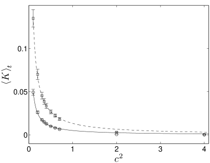
Figure 1: The variation of the spatial and time averaged kinetic energy $\left<K\right>_{t}$ with $c^{2}$ . The circle symbols are for Manneville’s model with parameters $\epsilon=0.7$, $\sigma=2$, $g_{m}=50$, and the square symbols are for the GSH equation with $\epsilon=0.7$, $\sigma=1$, $g_{m}=50$. The lines are curve fits given by $\left<K\right>_{t}=0.013c^{-2}$ for the GSH model and $\left<K\right>_{t}=0.005c^{-2}$ for Manneville’s model. The results are averaged using the last $10^{5}$ time units of a simulation with total time $t=10^{6}$. The error bars are the standard deviation of the fluctuations of $\left<K\right>_{t}$ about its mean value; their maximum values are $\sim 10^{-2}$ and $\sim 10^{-3}$ for the GSH model and Manneville’s model, respectively.

Figure 2 illustrates the pattern evolution for $c^{2}=2$ using Manneville’s model. The value of $c^{2}=2$ is the typical value used in the literature and corresponds to a weak mean flow. At small time $t=10^{3}$ the pattern is quite complex and contains many dynamic spiral and defect structures, similar to the scenario given in the simulations of Xi et al. Xi et al. (1993). The coarsening to target structures is evidenced by the pattern at $t=5\times 10^{4}$ and represents the approximate duration of the simulations by Schmitz et al. using the GSH equation Schmitz et al. (2002). This coarsening process is extremely slow as can be seen by comparing the patterns at longer times in Fig. 2 (the pattern at $t=10^{6}$ for these simulation parameters is shown in the bottom right panel of Fig. 3). Note that during the time evolution some big targets can break up and form small defects which will then interact and recombine with other targets or spirals, resulting in the process of coarsening.

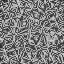
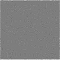
$t=1000$	$t=50,000$
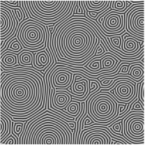
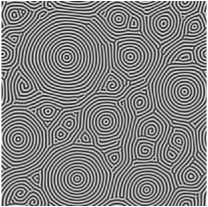
$t=100,000$	$t=200,000$

Figure 2: Instances of the $\psi$ field pattern for Manneville’s model with system parameters $\epsilon=0.7$, $\sigma=2$, $g_{m}=50$, and $c^{2}=2$, showing a slow process of pattern coarsening. Small spiral defects dominate at early times (e.g., $t=10^{3}$), whereas at large times the pattern has evolved into a state dominated by large and very slow moving target structures.

We have explored the long-time dynamics of the patterns by varying the strength of the mean flow over the parameter range of $0.1\leq c^{2}\leq 4$. Figure 3 illustrates the patterns at $t=10^{6}$ for four different values of $c^{2}$. For the cases shown, the patterns resemble the state of spiral defect chaos for $c^{2}\lesssim 0.7$, showing spatially complex structures with rapid dynamics of small-scale spirals and localized defects. Although during the evolution process some larger spirals or targets may be formed, they are transients and will soon break up, with new small spiral defects recreated; this procedure will repeat, but no long-lasting, coarsened big targets or spirals can exist. However, for larger $c^{2}$ (e.g., $=2$) the pattern has coarsened to a state dominated by slowly moving target defects, as the case given in Fig. 2. These observations indicate that strong enough mean flows, as achieved via controlling parameter $c^{2}$ in the model equations, are needed to reach a persistent chaotic or dynamic state, not only for breaking up large targets or spirals but also for locally recreating new small spiral-type defects to prevent the coarsening procedure.

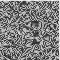
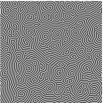
$c^{2}=0.1$	$c^{2}=0.5$
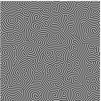
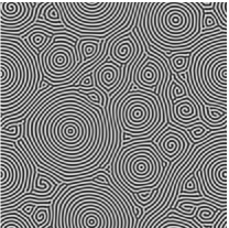
$c^{2}=0.7$	$c^{2}=2$

Figure 3: The long-time patterns for Manneville’s model over a range of mean flow strengths as determined by the value of $c^{2}$. The simulations are initiated with random initial conditions and are integrated until $t=10^{6}$. Other parameters are the same as Fig. 2.

To further characterize the properties of system dynamics, in Fig. 4 we examine the time variation of two global quantities: the average kinetic energy $K(t)$ as defined in Eq. (10), and the convective heat flux $J(t)$ which is given by

$$J(t)=\left<\psi^{2}\right>.$$ (11)

Fig. 4(a) indicates that as the strength of the mean flow increases (i.e., the values of $c^{2}$ decrease), the magnitude of the heat flux decreases with increasing fluctuations about the mean value. Such fluctuations are a result of the pattern dynamics. More specifically, the dynamics of the defects yield the excursions to larger and smaller values of the heat flux. For the average kinetic energy as shown in Fig. 4(b), both the magnitude of $K(t)$ and its fluctuations increase with increasing strength of the mean flow. Overall, Fig. 4 can be used to shed some qualitative insight upon the complexity of the dynamics. It is clear that for $c^{2}=2$ (which is the parameter used in most previous studies) the disorder in the kinetic energy and heat flux is significantly reduced.

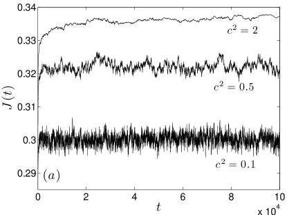
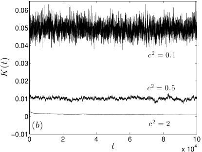
Figure 4: Time variation of the pattern dynamics in Manneville’s model for different magnitudes of the mean flow. The parameters used are the same as those in Fig. 3. (a) Time variation of the convective heat flux $J(t)$ given by Eq. (11); (b) Time variation of the average kinetic energy $K(t)$ defined by Eq. (10).

Although global diagnostics such as the kinetic energy and heat flux provide qualitative insights into the complexity of system dynamics, they can not be used to determine if the dynamics are chaotic. In order to determine if the dynamics are chaotic we have also calculated the finite-time leading order Lyapunov exponent using the approach discussed in Sec. II.2. In Fig. 5 we show the variation of $\lambda_{1}$ with the magnitude of the mean flow, for which $\lambda_{1}>0$ indicates chaos. The circle symbols are the results for Manneville’s model and the solid line is included only to guide the eye. We emphasize that these results are obtained from very long-time simulations to ensure that any slow coarsening dynamics have been captured. The reported values of $\lambda_{1}$ are computed using the final $10^{5}$ time units. The standard deviation of the fluctuations of $\lambda_{1}$ about its mean value is included as error bars. The maximum value of the error bar for the parameters explored is $\sim 10^{-3}$. We have also performed tests upon the data where $\lambda_{1}$ is computed over successive windows of time of various durations to quantify the presence of any slow trends. Our reported values of $\lambda_{1}$ appear to be the converged result and for the duration of the simulations explored we did not find any indication of slow trends. However, this does not rule out the possibility of even slower dynamics not captured in our simulations.

Our simulations indicate that the dynamics are weakly chaotic for $c^{2}\approx 2$ where $\lambda_{1}\approx 0.05$. This weak chaos is due to the slow dynamics of the pattern, as can be seen in Fig. 3 where the targets are slowly moving among the more rapid dynamics of defects such as spirals, dislocations, etc. The value of $\lambda_{1}$ increases with the decreasing value of $c^{2}$ and thus the increasing magnitude of the mean flow as given in Fig. 5.

We have also included in Fig. 5 the numerical results of the GSH equation to enable a more direct comparison with prior results in the literature. These results are shown as the square symbols and the dashed line. We have allowed $c^{2}$ to vary while the remaining parameters are the typical values used in the previous studies: $\epsilon=0.7$, $\sigma=1$, and $g_{m}=50$. Overall our results indicate a very similar trend: the dynamics are weakly chaotic for $c^{2}\approx 2$ and become increasingly chaotic for smaller $c^{2}$ and larger magnitudes of the mean flow. We have performed the same series of tests as for Manneville’s model to account for the presence of any slow coarsening process. The maximum magnitude of $\lambda_{1}$ error bars for the GSH equation is $\sim 10^{-2}$.

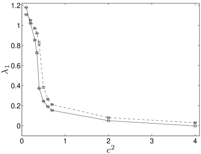
Figure 5: The variation of the leading order Lyapunov exponent $\lambda_{1}$ with the magnitude of the mean flow. The value of $\lambda_{1}$ is computed using results for the final $10^{5}$ time units. The circle symbols and the solid line are for Manneville’s model using the system parameters $\epsilon=0.7$, $\sigma=2$, and $g_{m}=50$. The square symbols and the dashed line are for the GSH equation using the typical system parameters of most previous studies: $\epsilon=0.7$, $\sigma=1$, and $g_{m}=50$. The lines are only meant to guide the eye. The error bars represent the standard deviation of $\lambda_{1}$ about its mean value for each value of $c^{2}$. The maximum value of the error bar for Manneville’s model is $\sim 10^{-3}$ and for the GSH equation is $\sim 10^{-2}$.

Although the connection between the Swift-Hohenberg equations and the Boussinesq equations of Rayleigh-Bénard is phenomenological, a direct comparison between the two can provide further physical insights. In this comparison we mainly focus on spatial features of the mean flow field for chaotic patterns containing a large number of spiral defects. In Fig. 6(a) we illustrate the relationship between the pattern and the magnitude of the mean flow. The image shown is for Manneville’s model at $t=10^{6}$ with $c^{2}=0.1$. The dynamics are chaotic with $\lambda_{1}\approx 1.2$ as given in Fig. 5. The color contours represent the magnitude of the mean flow field $|\mathbf{U}|$ where red indicates regions of large mean flow and blue indicates regions of small mean flow. The roll pattern is shown by the black lines which are given by contours of $\psi=0$. The mean flow tends to reach its local maximum at locations that contain defect structures and remains large on a length scale of several roll wavelengths around the defect.

We also performed numerical simulations of the three-dimensional time-dependent Boussinesq equations that describe Rayleigh-Bénard convection. We used a parallel spectral approach that is discussed in detail elsewhere (c.f. Paul et al. (2003)). We have chosen the reduced Rayleigh number $\epsilon=0.7$, the Prandtl number Pr=1, and an aspect ratio of $\Gamma=128$ for the spatial domain. The top and bottom boundaries have the no-slip fluid boundary condition and are held at constant temperature, while periodic boundary conditions are used on the sidewalls. The spatial variation of the mean flow is shown in Fig. 6(b). The mean flow is computed as the vertical average of the horizontal components of the fluid flow field, with red regions indicating large mean flow and blue regions corresponding to small mean flow. The black lines indicate the contours of the convection rolls. Due to the large aspect ratio of the domain the computational cost of the numerical simulation is considerable, and the image shown is for a time $t=232.9$ where $t$ has been nondimensionalized in the usual manner using the time for heat to diffuse across the depth of the layer. Qualitatively, the convective roll pattern is quite similar to what is shown for the Swift-Hohenberg-type equations. The spatial variation of the mean flow field, on the other hand, is different in terms of its rate of decay with the distance from a defect core. The mean flow field is largest at the core regions of the defect structures and decays rapidly with distance away from the defect core. In most cases the length scale of this decay is approximately that of a single roll (see Fig. 6(b)), as compared to several rolls for results of Manneville’s model shown in Fig. 6(a).

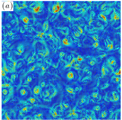
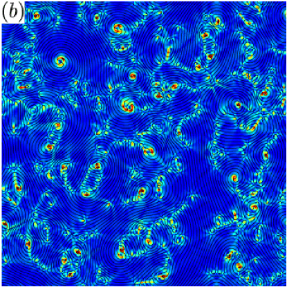
Figure 6: (color) Spatial variation of the mean flow field for chaotic patterns containing many spiral defects. The color contours represent the magnitude of the mean flow field, with red regions corresponding to large mean flow magnitude and blue regions corresponding to small mean flow magnitude. The black contours indicate convective roll boundaries. (a) Results for Manneville’s equations at $t=10^{6}$ using system parameters ($\epsilon=0.7$, $\sigma=2$, $g_{m}=50$, $c^{2}=0.1$). (b) Results for the Boussinesq equations using system parameters $\epsilon=0.7$, Pr$=1$, and $\Gamma=128$ at time $t=232.9$.

The derivation of the Swift-Hohenberg equations is based upon a long wavelength approximation and hence the corresponding results are not expected to be accurate in the core regions of defect structures Swift and Hohenberg (1977). This is illustrated in Fig. 7 which shows a close-up view of the mean flow structure near a spiral defect, with panel (a) for results of Manneville’s model and panel (b) for the Boussinesq equations. In both cases the spiral is rotating in a counter-clockwise direction. For the Swift-Hohenberg equations the mean flow exhibits a quadrupole structure centered upon the spiral. The magnitude of the quadrupole is spatially asymmetric and varies with the defect dynamics. The mean flow for the Boussinesq equations is a vortex rotating in the opposite direction to the rotation of the spiral. Our results for the Boussinesq equations are in agreement with those presented by Bodenschatz et. al (see Fig. 18 in Ref. Bodenschatz et al. (2000)).

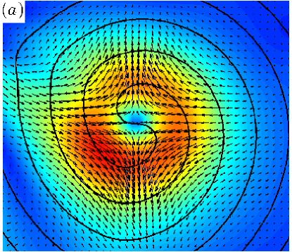
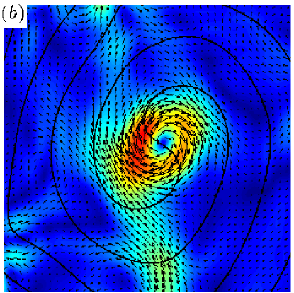
Figure 7: (color) A close-up view of the spatial variation of the mean flow near a spiral defect in a chaotic pattern. The color contours represent the magnitude of the mean flow as in Fig. 6, the black contours indicate the convective roll boundaries, and the arrows are vectors for the mean flow. (a) Results using Manneville’s equations with system parameters $\epsilon=0.7,\sigma=2$, $g_{m}=50$, and $c^{2}=0.4$ at time $t=7\times 10^{5}$. (b) Results from the Boussinesq equations using system parameters $\epsilon=0.7$, $\sigma=1$, and $\Gamma=128$ at time $t=232.9$.

IV Conclusion

Using generalizations of the Swift-Hohenberg equation we have explored the spiral defect chaos state and the role of the mean flow. Our results show that it is possible to generate chaotic dynamics using Swift-Hohenberg-type model equations that resemble the spiral defect chaos of Rayleigh-Bénard convection. The important insight is that the strength of the mean flow must be large enough. Reasonable parameter values of $\epsilon$, $\sigma$, and $g_{m}$ that lead to spiral defect chaos have been explored at some length in previous literature. However, the precise value of parameter $c^{2}$ depends on the approximations used in the derivation of Manneville’s equations and the appearance of $c^{2}$ is phenomenological in writing down the GSH equations. Our results show that the dynamics vary strongly with the magnitude of $c^{2}$ and the commonly used value of $c^{2}=2$ yields a mean flow that is not strong enough to generate persistent dynamics that resemble spiral defect chaos. By choosing a smaller value of $c^{2}$ the dynamics are chaotic for as long as we have simulated ($t=10^{6}$ time units). Although we focused our discussion upon results generated using Manneville’s equations, our conclusions and insights also apply to the GSH equations. The particular choice of the form of the nonlinearity does not strongly affect the results in any significant way that we have found. The necessity of a strong enough mean flow to support spiral defect chaos is in agreement with what has been found from the Boussinesq equations Chiam et al. (2003).

However, there are significant differences between numerical results from the Swift-Hohenberg-type model equations and those generated using the full three-dimensional Boussinesq equations. The Swift-Hohenberg equations are not expected to capture the small scale features correctly due to the long-wavelength approximation involved, and we have quantified some aspects of this by comparing the mean flow fields around a single spiral defect.

We anticipate that our results will have several uses. First is that Swift-Hohenberg-type equations can be used as a model to study spatiotemporal chaos in a system with direct relevance to fluid phenomena such as Rayleigh-Bénard convection. This is a significant advantage since numerical simulations of the Boussinesq equations are computationally very expensive Paul et al. (2003). The Swift-Hohenberg model equations could be used to explore fundamental ideas of spatiotemporal chaos that are currently inaccessible to the full fluid equations. Examples include a detailed study of microextensivity Tajima and Greenside (2002); Karimi and Paul (2010) or the computation of the characteristic Lyapunov exponents Gibbon et al. (2007); Pazó et al. (2008). In addition, our comparison of the spatial variation of the mean flow around spiral defect core structures could be used to guide the development of more accurate theoretical descriptions of spiral defect chaos.

Acknowledgments: MRP and AK acknowledge support from NSF grant no. CBET-0747727. Z-FH acknowledges support from NSF under Grant No. DMR-0845264.

References

- Cross and Hohenberg (1993) M. C. Cross and P. C. Hohenberg, Rev. Mod. Phys. 65, 851 (1993).
- Gollub and Ramshankar (1991) J. Gollub and R. Ramshankar, in New Perspectives in Turbulence, edited by L. Sirovich (Springer-Verlag, New York, 1991), p. 165.
- Skinner and Swinney (1991) G. S. Skinner and H. L. Swinney, Physica D 48, 1 (1991).
- Bar and Eiswirth (1993) M. Bar and M. Eiswirth, Phys. Rev. E 48, R1635 (1993).
- Bodenschatz et al. (2000) E. Bodenschatz, W. Pesch, and G. Ahlers, Annu. Rev. Fluid Mech. 32, 709 (2000).
- Morris et al. (1993) S. W. Morris, E. Bodenschatz, D. S. Cannell, and G. Ahlers, Phys. Rev. Lett. 71, 2026 (1993).
- Paul et al. (2003) M. R. Paul, K.-H. Chiam, M. C. Cross, P. F. Fischer, and H. S. Greenside, Physica D 184, 114 (2003).
- Swift and Hohenberg (1977) J. Swift and P. C. Hohenberg, Phys. Rev. A 15, 319 (1977).
- Xi et al. (1993) H. W. Xi, J. D. Gunton, and J. Viñals, Phys. Rev. Lett. 71, 2030 (1993).
- Schmitz et al. (2002) R. Schmitz, W. Pesch, and W. Zimmermann, Phys. Rev. E 65, 037302 (2002).
- Newell et al. (1990a) A. C. Newell, T. Passot, and M. Souli, J. Fluid Mech. 220, 187 (1990a).
- Newell et al. (1990b) A. C. Newell, T. Passot, and M. Souli, Phys. Rev. Lett. 64, 2378 (1990b).
- Manneville (1984) P. Manneville, in Cellular Structures in Instabilities, edited by J. Wesfreid and S. Zaleski (Springer-Verlag, 1984), vol. 210, pp. 137–155.
- Cross and Tu (1995) M. C. Cross and Y. Tu, Phys. Rev. Lett. 75, 834 (1995).
- Siggia and Zippelius (1981) E. D. Siggia and A. Zippelius, Phys. Rev. Lett. 47, 835 (1981).
- Manneville (1983) P. Manneville, J. de Physique 44, 759 (1983).
- Chiam et al. (2003) K.-H. Chiam, M. R. Paul, M. C. Cross, and H. S. Greenside, Phys. Rev. E 67, 056206 (2003).
- Huang and Viñals (2007) Z.-F. Huang and J. Viñals, Phys. Rev. E 75, 056202 (2007).
- Greenside and Cross (1985) H. Greenside and M. Cross, Phys. Rev. A 31, 2492 (1985).
- Cross et al. (1994) M. C. Cross, D. Meiron, and Y. Tu, Chaos 4, 607 (1994).
- Canuto et al. (1988) C. Canuto, A. Quateroni, and T. Zang, Spectral Methods in Fluid Dynamics (Springer-Verlag, Berlin, 1988).
- Cox and Matthews (2002) S. M. Cox and P. C. Matthews, J. Comp. Phys. 176, 430 (2002).
- Kassam and Trefethen (2005) A.-K. Kassam and L. N. Trefethen, J. Sci. Computing 26, 1214 (2005).
- Wolf et al. (1985) A. Wolf, J. Swift, H. L. Swinney, and A. Vastano, Physica D 16, 285 (1985).
- Bodenschatz et al. (1991) E. Bodenschatz, J. R. de Bruyn, G. Ahlers, and D. S. Cannell, Phys. Rev. Lett. 67, 3078 (1991).
- Cross (1996) M. C. Cross, Physica D 97, 65 (1996).
- Tajima and Greenside (2002) S. Tajima and H. S. Greenside, Phys. Rev. E 66, 017205 (2002).
- Karimi and Paul (2010) A. Karimi and M. R. Paul, Chaos 20, 043105 (2010).
- Gibbon et al. (2007) J. D. Gibbon, P. Poggi, A. Turchi, H. Chatè, R. Livi, and A. Politi, Phys. Rev. Lett. 99, 130601 (2007).
- Pazó et al. (2008) D. Pazó, I. G. Szendro, J. M. López, and M. A. Rodríguez, Phys. Rev. E 78, 016209 (2008).