Entanglement-assisted tomography of a quantum target
Abstract
We study the efficiency of quantum tomographic reconstruction where the system under investigation (quantum target) is indirectly monitored by looking at the state of a quantum probe that has been scattered off the target. In particular we focus on the state tomography of a qubit through a one-dimensional scattering of a probe qubit, with a Heisenberg-type interaction. Via direct evaluation of the associated quantum Cramér-Rao bounds, we compare the accuracy efficiency that one can get by adopting entanglement-assisted strategies with that achievable when entanglement resources are not available. Even though sub-shot noise accuracy levels are not attainable, we show that quantum correlations play a significant role in the estimation. A comparison with the accuracy levels obtainable by direct estimation (not through a probe) of the quantum target is also performed.
pacs:
03.65.Wj, 03.65.Nk, 06.20.Dk,72.10.-d1 Introduction
The possibility of reconstructing the quantum state of a system via measurements (quantum state tomography, QST) is a central problem in quantum information theory [1], which poses a series of fundamental questions related to the fact that the state itself is not directly observable and that each given quantum measurement typically reveals only partial information on the observed system. In recent years, a great deal of work has been devoted to this issue and many important features have been recognized, including the fact that having at disposal several copies (say ) of the initial state, collective measurements are more informative than individual ones, e.g., see Refs. [1, 2, 3] and references therein. In abstract terms, QST ultimately reduces to the ability of estimating the set of continuos parameters which define the expansion of an unknown state with respect to a reference basis of operators (say the set of Pauli matrices for a two-level system, qubit). As such, its ultimate accuracy limits can be evaluated by exploiting some general results of quantum estimation theory [4, 5, 9, 10] (more precisely, of a part of the theory which directly deals with the estimation of continuos parameters).
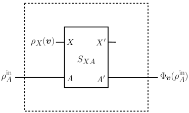
Up to date, most of the works focused on scenarios where the system under investigation can be directly accessed, i.e., posing no constraint whatsoever to the physical operations one may perform on it. In this context, for instance, the ultimately accuracy limit obtainable in the tomographic reconstruction of a qubit initialized in an arbitrary (possibly) mixed state have been set in Ref. [3], by computing the associated quantum Cramér-Rao (CR) bound [4, 5], in terms of the quantum Fisher information (QFI) matrix of the problem (see below for the precise definitions). In this paper, instead, we address the problem from a slightly different perspective, which captures an important aspect of many realistic experimental situations. More precisely, along the line set in Ref. [11], we consider the case in which the system of interest (from now on the target ), can only be addressed indirectly via measurements performed on a probe which has interacted with it. In our model the latter is described as a quantum system characterized both by external (e.g., momentum/position) and internal (e.g., spin) degrees of freedom, which the experimentalists are allowed to prepare in any initial configuration (also the target possesses external and internal degrees of freedoms but, for the sake of simplicity, only these last are supposed to be unknown, the external degrees of freedom being assigned by fixing the position of the target system). The tomographic reconstruction then proceeds by letting and interact via a scattering process and by measuring the final state of the former (or at least a part of it which has been scattered along some preferred direction). Indeed, the whole setting is devised in order to mimic the basic features of a standard (Rutherford-like) scattering experiment, where one tries to reconstruct the properties of a target system by firing probe particles on it and by looking at the way they emerge from the process. For the sake of simplicity we will limit the analysis to the case of 1D scattering processes, and describe the internal degrees of freedom of and as two-level (spin) systems (similar models have been recently analyzed to study entanglement generation [12, 13]).
It is worth noticing that the problem we are considering admits also an interpretation in the context of quantum channel estimation theory (see Ref. [10] and references therein). This is the theory, sometimes identified with the name of quantum metrology, which studies the efficiency of those schemes designed to recover information not on a quantum system, but on a quantum channel (quantum process tomography, QPT). We remind that in quantum mechanics quantum channels represent the most general physical transformations and are fully described by assigning completely-positive trace-preserving linear (CPTL) mappings [5], which act on the density matrices of the system (in our case the probe ). In quantum metrology the mapping is assumed to belong to a family of transformations identified by a set of parameters , whose values are unknown and which we wish to recover by preparing the system in some fiduciary initial state and by measuring the corresponding output state transformed by the channel. In our case the quantum channel to be estimated is the one that induces a modification on the probe via its interaction with the target , while the ’s correspond to the parameters that define the (unknown) state (see Fig. 1). In the jargon introduced in Ref. [15], this transformation belongs to the special class of programmable channels111Explicitly, these channels can indeed be parametrized by assigning a fixed interaction with an external unknown system. In a seminal paper [6] Nielsen and Chuang proved that the family of all unitaries acting on qubits is not programmable, since an -qubit register can encode at most distinct quantum operations. Notwithstanding the non-universality of programmable channels, the authors also pointed out the possibility to program the family of unitary operations probabilistically. In this context, an interesting model was proposed for the case of single qubits in [7] and implemented for photonic qubits in [8]..
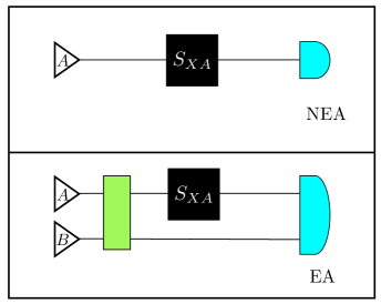
A well-known fact is that, in general, if is the number of tests we perform in order to recover the actual values of (each test consisting of applying the same channel to a new copy of probe ) the statistical scaling of the associated uncertainty can be reduced from the “standard quantum limit” (SQL) (or “shot noise” in quantum optics) scaling, to the so-called “Heisenberg bound” scaling, by the introduction of suitable quantum correlations between initializations of the various copies of [10, 14]. However, this is not the case if, as in our case, the channels under investigation are programmable [15]. As a consequence in our model no sub-shot noise scaling in of the accuracy should be expected. For this reason we will limit the analysis to those configurations in which the tests on are performed by preparing copies of in the same initial state. The QFI matrix approach [4, 5, 9] will then be used to evaluate the associated accuracy, optimizing it with respect to the initial preparation of (with respect to both its internal and external degrees of freedom) and comparing it with the results obtained in Ref. [3] for the case of direct estimation. Most importantly, we will also study an entanglement-assisted (EA) strategy, where each copy of is initialized into an entangled state of with an external ancilla system , which does not interact directly with (see Fig. 2), showing a clear improvement in the performance of the estimation process with respect to the non-EA (NEA) strategy in line with the findings of Refs. [14, 16].
The paper is organized as follows. In Sec. 2 we introduce our scattering model and briefly review some basic aspects of quantum estimation theory. Then, in Secs. 3 and 4 we will discuss two different strategies for the tomographic reconstruction of the target qubit, with and without the help of quantum correlations in the probe preparation. In particular, in Sec. 3 we first derive the exact expression for the QFI matrix in the case of an EA configuration, in which the probe is initialized in a maximally entangled state with the ancilla system, and discuss some applications of the result in the evaluation of some functionals of the state of the target (specifically its purity and its azimuthal angle). In Sec. 4, instead, we compare the EA and NEA cases by focusing on a special configuration in which the target state is characterized by a single unknown parameter. The paper ends with Sec. 5 by summarizing our results in the light of future perspectives. The more technical aspects of the derivation are presented in a couple of appendices.
2 The model
In this section we introduce the model and set up the notation.
2.1 1D scattering of the probe
Suppose that a target qubit is fixed at a given position on a line, and that its unknown state is described by the density matrix
| (1) |
with being the Pauli operators, and the 3D Bloch vector, which represents the set of parameters we wish to recover via QST. In Ref. [11] it was shown that [and hence ] can be obtained from the transmission and reflection probabilities of a probe qubit scattered off through a point-like interaction, which couples the internal degrees of freedom of the two qubits via the following Heisenberg-type Hamiltonian
| (2) |
Here, and are the mass and the momentum operators of , is a positive coupling constant, and are the Pauli operators acting on the qubit . Specifically, in Ref. [11] was assumed to be initialized into a known input state and injected from the left of the line with momentum . This kind of systems can be considered as models for a magnetic impurity spin embedded along a 1D wire [17], such as a semiconductor quantum wire [18] or a single-wall carbon nanotube [19]. For instance, an electron is sent through the 1D wire as a probe particle, and its spin state is resolved after the scattering by spin-sensitive filters [20]. Alternatively, an electron populating the lowest subband of the 1D wire can undergo scattering from two double quantum dots [21] to which it is electrostatically coupled. The state tomography of then proceeded by solving the associated scattering problem and looking at the state of which emerges either on the left (transmitted component) or on the right (reflected component), or both. Such states admit a simple expression in terms of the scattering matrix of the process defined by the unitary operator
| (3) |
with
| (4) |
Here the ’s represent the momentum eigenstates of the probe ( being the associated eigenvalues), while the matrices and define the spin-dependent scattering amplitudes associated with transmission and reflection events, respectively. They are functions of the probe wave number and are given by
| (5) |
with being the dimensionless parameter
| (6) |
and
| (7) | |||
| (8) |
For an explicit derivation of all these equations we refer the reader to [11].
Consider now an experimental setting in which an observer tries to reconstruct by merging incoherently222 By incoherent merging of the transmitted and reflected data, we mean that no joint measurements are allowed on the transmitted and reflected signals (a scenario which is realistic if the rhs and lhs detectors are located sufficiently apart from each other). the data associated with the transmission events (to the right of the target) and the reflection events (to the left). The final state of can be expressed as the tensor product of effective qutrit density operators
| (9) | |||||
where is the partial trace over , and () is a vector orthogonal to all the internal spin states of , which represents the vacuum state associated with no particle reaching the rhs (lhs) detector. The first term represents the contribution associated with a transmitted reaching the rhs detector (vacuum on the lhs), while the second represents the opposite one (i.e., spin on the lhs and vacuum on the rhs). The detectors are assumed to have 100% efficiency and no particle creation or destruction by the target is possible, so that the number of particles is conserved: every incident particle emerges either from the left or from the right of the target.
On the other hand, if the observer collects only transmitted particles, emerging from the rhs of the target, he will either see nothing ( being reflected by ) or see emerging with the same momentum it had when entering the line but with a modified spin state due to the interaction with . Such configuration is described by the density operator, obtained from by tracing out the reflected case, namely,
| (10) | |||||
Notice that here
| (11) |
is the reflection probability (i.e., the probability of no detection of on the rhs of the line).
An analogous expression holds for the alternative experimental setting in which the observer only collects information of the signals emerging from the lhs of the line. In this case Eq. (10) is replaced by
| (12) | |||||
The output density matrices , associated with the three different experimental settings, are functions of the state of . Therefore, one can acquire information on the latter by performing QST on the former. Furthermore, since also depends on the input state and on the input momentum of the probe , one can try to optimize the resulting accuracy with respect to these parameters.
2.2 Entanglement-assisted scheme
An interesting variation of the previous schemes is obtained by considering the case in which is prepared into a joint (possibly entangled) state with an ancilla system , that is not directly interacting with (see Fig. 2). Such EA configurations proved to be successful in boosting the efficiency of several quantum estimation [16] and discrimination schemes [23].
2.3 The Cramér-Rao bound
In the following sections we will compare the accuracy one can get by reconstructing through the EA configurations via measurements on the output states defined by the Eqs. (13), (14) and (15), with the corresponding accuracy one achieves with the NEA configurations associated with the output states of Eqs. (9), (10) and (12). Differently from [11] but in line with the approach of [3, 9], such accuracies will be evaluated by computing the corresponding quantum CR bounds [4, 5, 9].
We remind that the quantum CR theorem establishes a fundamental lower bound on the uncertainty of any estimation strategy devised to recover the three components of . Specifically, assume that one has copies of the state which encodes such parameters. (In our case, for the NEA setting is given by the states , depending on whether the observer collects only transmitted data, reflected data, or both. Similarly for the EA setting, where is identified with ). A generic estimation strategy consists in assigning a (possibly joint) POVM measurement on the copies of the state, and a classical data processing scheme that starting from the measurement outcome produces an estimation of the parameters . The uncertainty of the estimation can then be evaluated by means of the covariance matrix () obtained by averaging the distances between the real value of the parameter and their estimations. In this context the CR bound implies that, independently from the adopted POVM and classical data processing scheme, such matrix must verify the inequality
| (16) |
where is the QFI matrix of the encoding state [4, 9], i.e.,
| (17) |
Here, is the spectral decomposition of the encoding state , while stands for the partial derivative with respect to the th component of the vector . The th diagonal element of the inequality (16) provides the CR bound for the variance associated with the accuracy in the estimation of the parameter , for fixed values of the others, i.e.,333 Indeed, one can easily verify that the quantity coincides with the QFI function associated with the estimation of the parameter on the one-parameter family of states obtained from when assigning fixed values to the other components of .
| (18) |
(notice the SQL scaling of ). It is worth observing that even though the bound (16) is not always attainable, the bound (18) is known to be asymptotically achievable for a sufficiently large . More generally, Eq. (16) permits also to derive an accuracy bound on the variance of the estimation of any given function of the parameters [4, 9]. Specifically by re-parameterizing the problem with a new set of independent parameters , which include the quantity of interest as (say) the first element , one gets,
| (19) |
where is the QFI matrix of the parameters obtained from via the similarity transformation induced by the Jacobian matrix . As in the case of Eq. (18), for fixed values of and the inequality (19) establishes a bound on the accuracy reachable in the estimation of the function (the bound being achievable for a sufficiently large under the assumption that and are known a priori).
As an application of the above construction, and for future reference, it is instructive to report the quantum CR bounds associated with a direct estimation of which has been first computed in Ref. [3]. In this scenario the observer is assumed to have complete (not probe-mediated) access to the target state , so that the encoding state introduced above coincides with the density matrix . In this case the QFI matrix possesses a simple form in polar coordinates,
| (20) |
where it is diagonal. Indeed using Eq. (17) one finds,
| (21) |
where is the QFI matrix given by
| (22) |
with
| (23) |
Notice that the matrix does not depend upon the azimuthal angle while it is a function of the radial coordinate and on the polar angle (the latter however is just a geometric artifact introduced by the polar coordinates: the north and south poles are indeed insensitive to rotations along the -axis).
3 Entanglement-assisted strategy
In this section we will consider the case in which the probe is prepared in an entangled state with the ancilla , that is the EA strategy introduced in the previous section and represented in Fig. 2. More precisely, we will assume that subsystem before the scattering is in a maximally entangled state, and compute the analytic expression for the associated QFI matrix as a function of the set of parameters defining the initial state of and of the incident momentum of . In A we will prove that our results are independent on the specific choice of the maximally entangled input state of . Henceforth we will set the input state in the singlet state:
| (24) |
3.1 Collecting data in reflection and in transmission
Let us focus first on the experimental setting in which the observer collects both transmitted and reflected signals of the probe .
From the expression (17) of the QFI matrix it immediately follows that the reflection and transmission components of the state defined in Eq. (13) provide two separate contributions, as they are associated to orthogonal subspaces. Also, as in the case of the direct estimation discussed in the previous section, it turns out that the QFI matrix possesses a simple form in polar coordinates, where it is diagonal independently of the initial state of . Indeed, upon diagonalization of the state (13) we find that in this case the inequality (21) gets replaced by
| (25) |
where the QFI matrix is
| (26) |
with
| (27) | |||||
| (28) |
(in B we also report the expression of the bound in cartesian coordinates). As in the case of the direct estimation, does not depend upon the azimuthal angle , while it is a function of the radial coordinate and the polar angle . Such a behavior is associated with the symmetry of the coupling Hamiltonian (2), which does not possess a preferred spatial direction, and of the input state of .444We stress that the dependence of on has nothing to do with the probe-target coupling: as in the case of it is a geometric artifact of the polar representation. It is also worth pointing out that the matrix vanishes when is zero or infinite (that is, infinite or zero incident momentum of the probe ). This implies that for such configurations no recovering of information on is possible. Indeed if it means that is initially at rest and will not be able to be scattered by , while for very large it means that propagates so fast along the line that the interaction with can only have a minimal (asymptotically vanishing) impact on its evolution.
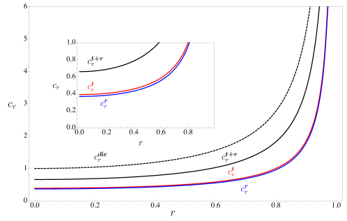
As a specific example suppose then that the observer, already knowing the value of the parameters and , is interested in recovering the missing parameter , which determines the purity of the target system , . Equation (25) then yields
| (29) |
which should be compared with the quantity one obtains in the direct estimation case, i.e., Eqs. (21)–(23). Since the rational function of on the rhs of Eq. (29) is larger than , it follows that is always smaller than the EA bound (this is very much expected since in the case of direct estimation the observer has access to the system, while in the EA strategy he can only recover info on through the probe ). The minimum of the rhs Eq. (29) is reached when as shown in Fig. 3, this value provides the optimal input momentum of via Eq. (6), for recovering the parameter . For such a choice the EA strategy misses the direct estimation accuracy just by a factor of . Notice finally that for both the EA strategy and for the direct one, the accuracy bounds vanish with the distance from the surface of the Bloch sphere (this is a consequence of the fact that it is intrinsically simpler to distinguish pure states from mixed states).

Consider next the case in which the observer, already knowing the value of the parameters and , is interested in recovering the azimuthal phase of the target system . This is given by the third diagonal element of the QFI matrix (26), i.e.,
| (30) |
which again should be compared with the bound one gets for the direct estimation. Again one can verify that the rhs of Eq. (30) is always larger than the direct estimation threshold (notice however that both expressions diverge for and due to fact that for such choices the variable is not even defined). For the sake of simplicity we focus on the special case in which is in a pure state on the equatorial plane of the Bloch sphere (i.e., and ). In this case Eq. (30) yields
| (31) |
which reaches its minimum when , where the rhs is , falling short of the direct threshold by 35%.
3.2 Collecting only reflected or transmitted data
By repeating the same analysis for the case in which only transmitted or reflected probes are detected (see Eqs. (14) and (15)) we find that Eq. (25) still holds with the QFI matrix being replaced by
| (32) |
with
| (33) | |||||
| (34) |
in transmission, while
| (35) | |||||
| (36) |
in reflection.
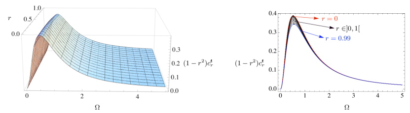
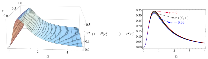
Notice that, in this case, even if there is still a quadratic divergence of and at , their dependence on does not factorize. Hence
in the estimation of the radius , the bound (29) is replaced by a lower bound, ,
which for every value of admits an optimal momentum for the incident probe that maximizes the associated QFI, as shown in Figs. 4 and 5.
Interestingly enough, however, there exist “optimality intervals” for the incident momentum (i.e., for transmission, and for reflection), which
guarantee rather high performances for all values of .
Observe that in order to achieve the optimal estimation from transmitted data we have to send the probe faster than the case of reflection (recall that ): this is in perfect agreement with the intuitive idea that to efficiently collect the data in transmission
should be given a sufficiently large initial momentum to prevent back scattering from
(and vice versa for reflection). Between the above two intervals lies the optimal value of for the case in which we collect all scattering data, .
In Fig. 6 we plot the QFI of the radius (purity) for the case of transmitted, reflected, or both reflected and transmitted data. Of course, the last case leads to the best estimation of the target purity, as we are collecting the largest amount of information from the scattering process.
Analogous considerations apply also to the estimation of the azimuthal angle . One can easily extract them by a direct comparison of the coefficients (34) and (36) with the corresponding expression associated with the transmission and reflection strategy given in Eq. (28) and also with the direct estimation procedure [see Eq. (23)].
4 Comparing EA and NEA strategies
In this section we will present a comparison between the EA strategies introduced in the previous section with the NEA strategies obtained by restricting the analysis to the case in which the initial state of the probe and the ancilla is separable. For the sake of simplicity, we find it instructive to restrict the analysis to the situation in which, as in Fig. 6, the observer aims only to estimate the purity of the target state . Specifically we will work under the assumption that the three dimensional vector which specifies in the Bloch sphere lies on the axis, that is and
| (37) |
Under this condition the quantum CR bound (16) reduces to an inequality for the variance of the unique parameter , i.e.,
| (38) |
where are the QFI functions of the problem computed as usual by exploiting the spectral decomposition of the output states and using Eq. (17) (which in this case contains only derivatives with respect of the unique parameter ).
For the EA configuration the functions coincide with the third diagonal elements of the QFI matrices in cartesian coordinates evaluated at , namely,
| (39) | |||||
| (40) | |||||
| (41) |
Notice that the above expressions can be retrieved from Eqs. (27), (33) and (35) by substituting with . The general expression of the QFI matrix for the EA configuration can be found in B.
Before computing the QFI functions for the NEA configuration, it is worth observing that due to the convexity of the QFI function (e.g., see Ref. [16]), it follows that in the NEA scenario the contribution of the ancilla in the scattering can be completely neglected, see Fig. 2. Indeed, since the maximum of a QFI function is always achieved on pure states, one can restrict the analysis of the NEA configuration to pure separable states of : for them however the output states of also factorize and one can completely ignore the subsystem . Consequently, the states of the system after the scattering are given by Eqs. (9), (10) or (12), for the case in which we collect either all scattering data, or only transmitted/reflected probes. In particular we will assume
| (42) |
where, without loss of generality, the input azimuthal angle has been set to zero by using the symmetry of the coupling Hamiltonian.
Let us then consider first the accuracy achievable when collecting data only on transmission, i.e., assuming as output state the one given in Eq. (10). The resulting QFI is the following (involved) function of :
| (43) | |||||
Still one recognizes some general features we already observed in the previous section. In particular the QFI function vanishes at and . Notice also that when the target state is pure, there exists a particular choice of the initial state of the probe such that the above quantity diverges quadratically, as found for the EA strategy, namely and , and arbitrary (finite) . Finally, notice that for each value of there exists an optimal point for the pair that maximizes the QFI.

In Fig. 7 we plot the envelope of the QFI for , that is the maximum value of , which can be proved to be a symmetric function of . Notice that the initial state of that yields the best estimation of the target state depends on , that is, on the initial state of the target, which is in principle unknown. We can only say that once we have set the direction of the probe in the Bloch sphere before the scattering, the best optimization we can get involves pure target states with Bloch vectors parallel to this direction. The same analysis can be repeated for reflection and yields:
| (44) |
Similarly to the case of transmission the optimal values of and are symmetric functions of . Moreover, when the target state is pure, i.e., and , the QFI diverges for and , respectively, as for transmission.
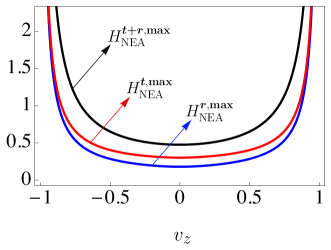
Finally, the largest amount of information on the system can be inferred by collecting both transmitted and reflected data. In this case the QFI associated to the state (9) of the incident probe after the scattering is given by
| (45) |
This function exhibits the same properties as and . The three curves plotted in Fig. 8, all symmetric with respect to , refer to the optimal values of the QFI for the three cases analyzed above. As expected, the collection of all scattering data returns the best tomographic reconstruction of the target state. Notice that the transmission strategy seems to overcome the reflection one, like in the EA strategy. Also it can be shown that for all the optimal value of for the transmission is lower than that for reflection, and for the case in which we collect both transmitted and reflected data it is in between (this results have been obtained by numerical optimizations).
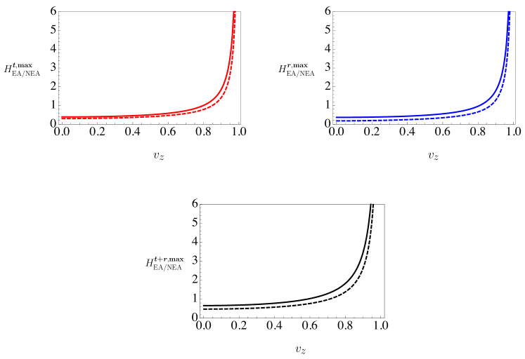
In order to compare the efficiency of the NEA strategies with the EA strategies discussed in the previous section, in Fig. 9 we plot the maximum QFI for , for the EA (solid line) and the NEA (dashed line) strategies (the expression for the EA strategies have been obtained by exploiting the representation of the QFI matrix in cartesian coordinates reported in B). The role played by the entanglement between the probe and the ancilla before the scattering is evident: it implies an enhancement in the QFI for all , both for the case in which we collect all the scattering data and for the case in which we have access only to trasmission/reflection events.
5 Conclusion
We have presented a detailed study of the tomographic state reconstruction of a target system, obtained by monitoring a scattered probe. Focusing on the special case in which both the target and the probe are qubit systems, and assuming the scattering to take place on a 1-D line, we used quantum estimation techniques to evaluate the efficiency of the process in several configurations of interest. In particular we distinguished two regimes: the EA regime in which the observer is allowed to initialize the probe in an entangled state with an external ancilla that it is kept in the laboratory; and the NEA regime where instead no entanglement is allowed between the probe and the ancilla. As expected, when all the other settings are kept identical, the EA strategies turn out to be more effective then their NEA counterparts.
Within both regimes we have also studied what happens when the observers have access to all or only part of the scattered data. Specifically we consider the cases in which only transmitted or reflected data are used in the tomographic reconstruction, noticing that these regimes are characterized by different optimal values for the input momentum of the probing particle (the transmitted scenario being characterized by higher optimal input momenta than the reflected one). We have also analyzed the situation in which both transmitted and reflected data are available to the observer, assuming though that no joint coherent measurements could be performed on the associated quantum degree of freedom (i.e. we explicitly excluded the possibility of performing joint detection on the left and right side of the 1-D channel, an hypothesis which is very much reasonable if the detectors are located at sufficient large distances from each other). The overall accuracy clearly benefits from this possibility: still it remains below the threshold [3] one gets when direct access to the target system is allowed. An open problem is to the determine whether or not one could exploit other sort of quantum resources to close such gap. A possible candidate which we aim to explore in a future development of the work, is to allow the observer to entangle different probes together (in the present scenario indeed, even though we used probes, they were all prepared in a factorized configuration of the same initial state). This strategy could in fact benefit from super-additivity effects arising from the presence of non classical correlations between the various probes, resulting in higher performances of the tomographic reconstruction. An interesting open problem is also to understand to what extend the specific features we have observed in our simple scattering model (qubits interacting along a 1-D line via Heisenberg-like coupling) could be generalize to more complex configurations (say by increasing the size the of the target and/or of the probe, or by allowing the scattering to take place in a 2-D or a 3-D setting).
This work was supported by the Italian Ministry of University and Research through FIRB-IDEAS Project No. RBID08B3FM as well as under the bilateral Italian-Japanese Projects II04C1AF4E on “Quantum Information, Computation and Communication,” by the Joint Italian-Japanese Laboratory on “Quantum Information and Computation” of the Italian Ministry for Foreign Affairs, and by a Special Coordination Fund for Promoting Science and Technology and a Grant-in-Aid for Young Scientists (B) (No. 21740294) both from the Ministry of Education, Culture, Sports, Science and Technology, Japan.
Appendix A Equivalence between maximally entangled states
We explicitly prove that our analysis for the EA strategies is independent of the particular choice of a maximally entangled state for the subsystem .
The Heisenberg-type coupling describing the interaction between qubits and can be written in terms of the so-called swap operator as
| (46) |
It is a unitary self-adjoint operator and is characterized by the following very simple property
| (47) |
where and act in the same way on and , respectively (), and is the swap operator in the rotated frame
| (48) |
The above property is trivially conserved for the interaction Hamiltonian . The equivalence among all the maximally entangled input states for the EA strategies is thus straightforward. Indeed, a generic maximally entangled state of the probe and the ancilla can always be written as , with the singlet state (24). If we send to the target qubit it can be easily shown that the contributions given by in the final state of the subsystem become
with
Since the physical properties of the system do not depend on the choice of the reference basis, the results of our analysis for the EA strategies are completely independent of the choice of an initial maximally entangled state of .
Appendix B QFI matrix in cartesian coordinates
In this appendix we consider the explicit expression of the Fisher matrix for the EA strategy and discuss the symmetry properties of its elements.
For the case in which both transmitted and reflected probes are collected, the off diagonal elements of the Fisher matrix are given by
| (49) |
with , while for the diagonal elements we have
| (50) |
with . Notice that if there is only one out of the three parameters characterizing the initial state of the target different from zero, and , the QFI matrix is diagonal and thus its element coincides with the single parameter QFI for . Furthermore, due to the symmetry of the Heinsenberg-type interaction and of the singlet state of and before the scattering, we find
| (51) |
If we are able to detect only transmitted or reflected probes we get
| (52) | |||
| (53) |
and
| (54) | |||
| (55) |
. Analogously to the case in which we detect all the scattered probes, we find that also for the transmission and the reflection cases if we have and , , the QFI for is diagonal, and furthermore an equation similar to (51) holds:
| (56) |
References
- [1] Paris M G A and Řeháček J (eds) 2004 Quantum State Estimation (Berlin: Springer)
- [2] Peres A and Wootters W K 1991 Phys. Rev. Lett. 66 1119 Jones K R 1994 Phys. Rev. A 50 3682 Massar S and Popescu S 1995 Phys. Rev. Lett. 74 1259 Brodyand D and Meister B 1996 Phys. Rev. Lett. 76 1 Gill R D and Massar S 2000 Phys. Rev. A 61 042312 Hradil Z, Summhammer J, Badurek G and Rauch H 2000 Phys. Rev. A 62 014101 Bagan E, Baig M, Brey A, Muñoz-Tapia R and Tarrach R 2000 Phys. Rev. Lett. 85 5230 Massar S 2001 Phys. Rev. A 62 040101(R) Bagan E, Baig M, Brey A, Muñoz-Tapia R and Tarrach R 2001 Phys. Rev. A 63 052309 Peres A and Scudo P F 2001 Phys. Rev. Lett. 86 4160 Bagan E, Baig M and Muñoz-Tapia R 2001 Phys. Rev. A 64 022305 Banaszek K and Devetak I 2001 Phys. Rev. A 64 052307 Matsumoto K 2002 J. Phys. A 35 3111 Hannemann Th, Reiss D, Balzer Ch, Neuhauser W, Toschek P E and Wunderlich Ch 2002 Phys. Rev. A 65 050303 Bagan E, Baig M and Muñoz-Tapia R 2002 Phys. Rev. Lett. 89 277904 Embacher F and Narnhofer H 2004 Ann. Phys. 311 220 Bagan E, Monras A and Muñoz-Tapia R 2005 Phys. Rev. A 71 062318
- [3] Bagan E, Ballester M A, Gill R D, Monras A and Muñoz-Tapia R 2006 Phys. Rev. A 73 032301
- [4] Helstrom C W 1976 Quantum Detection and Estimation Theory (New York: Academic Press)
- [5] Holevo A S 2011 Probabilistic and Statistical Aspects of Quantum Theory 2nd edn (Pisa: Edizioni della Normale, 2011)
- [6] Nielsen M A and Chuang I L 1997 Phys. Rev. Lett. 79 321
- [7] Vidal G, Masanes L and Cirac J I 2002 Phys. Rev. Lett. 88 047905
- [8] Micǔda M, Ježek M, Dušek M and Fiurášek J 2008 Phys. Rev. A 78 062311
- [9] Paris M G A 2009 Int. J. Quant. Inf. 7 125
- [10] Giovannetti V, Lloyd S and Maccone L 2011 Nature Photo. 5 222
- [11] De Pasquale A, Yuasa K and Nakazato H 2009 Phys. Rev. A 80 052111
- [12] Ciccarello F, Palma G M, Zarcone M, Omar Y and Vieira V R 2006 New J. Phys. 8 214 Ciccarello F, Paternostro M, Kim M S and Palma G M 2008 Phys. Rev. Lett. 100 150501 Ciccarello F, Paternostro M, Palma G M and Zarcone M 2009 New J. Phys 11 113053 Ciccarello F, Paternostro M, Bose S, Browne D E, Palma G M and Zarcone M 2009 Phys. Rev. A 82 030302(R) Cordourier-Maruri G, Ciccarello F, Omar Y, Zarcone M, de Coss R and Bose S 2010 Phys. Rev. A 82 052313
- [13] Yuasa K and Nakazato H 2007 J. Phys. A 40 297 Yuasa K, Burgarth D, Giovannetti V and Nakazato H 2009 New J. Phys. 11 123027 Yuasa K 2010 J. Phys. A 43 095304
- [14] Giovannetti V, Lloyd S and Maccone L 2006 Phys. Rev. Lett. 96 010401
- [15] Ji Z, Wang G, Duan R, Feng Y and Ying M 2008 IEEE Trans. Inf. Theory 54 5172
- [16] Fujiwara A 2001 Phys. Rev. A 63 042304 Fisher D G, Mack H, Cirone M A and Freyberger M 2001 Phys. Rev. A 64 022309 Sasaki M, Ban M and Barnett S M 2002 Phys. Rev. A 66 022308 Fujiwara A and Imai H 2003 J. Phys. A 36 8093 Ballester M 2004 Phys. Rev. A 69 022303
- [17] Costa A T Jr., Bose S and Omar Y 2006 Phys. Rev. Lett. 96 230501
- [18] Datta S 1997 Electronic Transport in Mesoscopic Systems (Cambridge: Cambridge University Press) Harrison P 2005 Quantum Wells, Wires and Dots 2nd edn (West Sussex: Wiley) Gunlycke D, Jefferson J H, Rejec T, Ramšak A, Pettifor D G and Briggs G A D 2006 J. Phys.: Condens. Matter 18 S851
- [19] Tans S J, Devoret M H, Dai H, Thess A, Smalley R E, Geerligs L J and Dekker C 1997 Nature 386 474
- [20] Kawabata S 2001 J. Phys. Soc. Jpn. 70 1210
- [21] Hayashi T, Fujisawa T, Cheong H D, Jeong Y H and Hirayama Y 2003 Phys. Rev. Lett. 91 226804 Gorman J, Hasko D G and Williams D A 2005 Phys. Rev. Lett. 95 090502
- [22] Cramér H 1946 Mathematical methods of statistics (Cambridge: Princeston University Press)
- [23] Sacchi M F 2005 Phys. Rev. A 71 062340 Sacchi M F 2005 Phys. Rev. A 72 014305 Tan S-H, Erkmen B I, Giovannetti V, Guha S, Lloyd S, Maccone L, Pirandola S and Shapiro J H 2008 Phys. Rev. Lett. 101 253601